Modelling the strongest silicate emission features of local type 1 AGNJournal: ApJ
Abstract
We measure the 10 and m silicate features in a sample of 67 local () type 1 active galactic nuclei (AGN) with available Spitzer spectra dominated by non-stellar processes. We find that the m silicate feature peaks at m with a strength (Sip = ln fp(spectrum)/fp(continuum)) of , while the m one peaks at m with a strength of . We select from this sample sources with the strongest 10m silicate strength (, 10 objects). We carry out a detailed modeling of the IRS/Spitzer spectra by comparing several models that assume different geometries and dust composition: a smooth torus model, two clumpy torus models, a two-phase medium torus model, and a disk+outflow clumpy model. We find that the silicate features are well modeled by the clumpy model of Nenkova et al. 2008, and among all models those including outflows and complex dust composition are the best (Hoenig et al. 2017). We note that even in AGN-dominated galaxies it is usually necessary to add stellar contributions to reproduce the emission at the shortest wavelengths.
Keywords:
(galaxies:) active: general galaxies: infrared: galaxiesI Introduction
A dusty torus surrounds the central engine of active galactic nuclei (AGN) on a scale of few pc (Krolik & Begelman 1988; Antonucci 1993; Robson et al. 1995; Peterson 1997, e.g.,). It shines at infrared (IR) wavelengths between 1 to 1000 m peaking at around 20 m (Sanders et al. 1989; Elvis et al. 1994, e.g,). This emission is the result of the IR re-radiation of optical-UV light generated around the central black hole (BH) that has been absorbed by the dusty torus (Neugebauer et al. 1979). The main observational components that describe it are the slope of the spectral energy distribution (SED) between 1-8 m, and the strength of the silicate features around 10m and 18m, that are produced within the warm dust of the torus that the AGN directly illuminates. The silicate features have been observed mostly in emission with the mid-infrared (MIR) infrared spectrometer (IRS) Spitzer in type 1 AGN (Siebenmorgen et al. 2005; Hao et al. 2005; Hatziminaoglou et al. 2015). In these AGN the 10m silicate feature is broader and peaks at much longer wavelengths ( m) than the “normal” silicate emission feature of the Galactic inter-stellar medium (ISM) (Hao et al. 2005; Siebenmorgen et al. 2005; Sturm et al. 2005; Li et al. 2008, e.g,). This suggests different silicate compositions, such as a different proportion and/or size of grains (Shi et al. 2006; Li et al. 2008, e.g.,).
Martínez-Paredes et al. 2017 used the starburst-subtracted IRS/Spitzer spectra of 20 quasi stellar objects (QSOs) between to 15 m plus the unresolved near-infrared (NIR) emission to constrain the parameters of the dusty torus using the CLUMPY models of Nenkova et al. 2008a; Nenkova et al. 2008b. They noted that in most cases the spectral range around 8m is underestimated by the CLUMPY models and that trying to fit this part of the spectrum resulted in a bad fit of the silicate feature at 10m. Furthermore, in most cases the peak of the 10m silicate feature was shifted from the model location.
Considering that the shape and peak of the silicate features are strongly correlated with the properties of the dust (Draine et al. 2007; Sirocky et al. 2008, e.g.,), in this work we use five of the most popular torus models to investigate how well they reproduce the strongest silicate emission features observed in type 1 AGN. Recently, González-Martín et al. 2019a compared these models and found that they can be distinguished according to the continuum slopes and silicate strengths, and in a second work (González-Martín et al. 2019b) they used MIR spectroscopy data of type 1 and type 2 AGNs in the Swift/BAT survey to investigate how these models reproduce their spectral continuum. We focus our study on type 1 AGN with strong silicate emission features because: 1) for type 2 AGN, the inclusion of a fraction () of silicate grains, either based on Draine 2003 or Ossenkopf et al. 1992 are enough to reproduce the observed silicate features in absorption (Ramos Almeida et al. 2011; Alonso-Herrero et al. 2011; Martínez-Paredes et al. 2015, see e.g.,); and 2) the silicate features are well above the continuum in the low resolution Spitzer spectra, which support the interpretation that the silicate features are due to AGN activity.
In this paper we aim at exploring how accurately smooth, clumpy, two-phase, and outflow torus models reproduce the IRS/Spitzer spectra of these objects, and analyzing the results in terms of physical differences like the geometry and dust composition assumed. The first model that we consider is the smooth torus model of (Fritz et al. 2006, Fritz06 hereafter), which assumes a continuous distribution of dust composed of graphite and silicate grains in almost equal percentages. The second model is the CLUMPY torus model of (Nenkova et al. 2008a; Nenkova et al. 2008b, Nenkova08), which assumes a standard ISM dust composition of silicates and graphite with sizes between 0.025 and 0.25 m. The third torus model is clumpy (Hönig & Kishimoto 2010b, Hoenig10) and assumes three dust components that include the standard ISM composition, the standard ISM composition with larger grains (0.1 - 1.0 m), and a larger fraction of graphite grains ( silicates and graphite, with sizes between 0.05 and 0.25 m). The fourth model (Hönig & Kishimoto 2017, Hoenig17) has two components: a dusty clumpy disk that takes into account the emission from the hotter dust close to the central engine; and a hollow cone formed by a wind of clumpy dusty clouds elongated toward the polar direction. This model assumes that the wind is originated close to the sublimation zone of the dusty disk. Because of that, the dust in the wind has similar properties to the dust in the sublimation zone.
The paper is organized as follows: in Section 2 we present our sample selection and data; in Section 3 we describe the models; in Section 4 we present the analysis; and in Section 5 the discussion. Our summary and conclusions are presented in Section 6. We adopt the following cosmology: H0 = 73 km s-1 Mpc-1, and .
II The sample and data
II.1 The silicate dominated local AGN
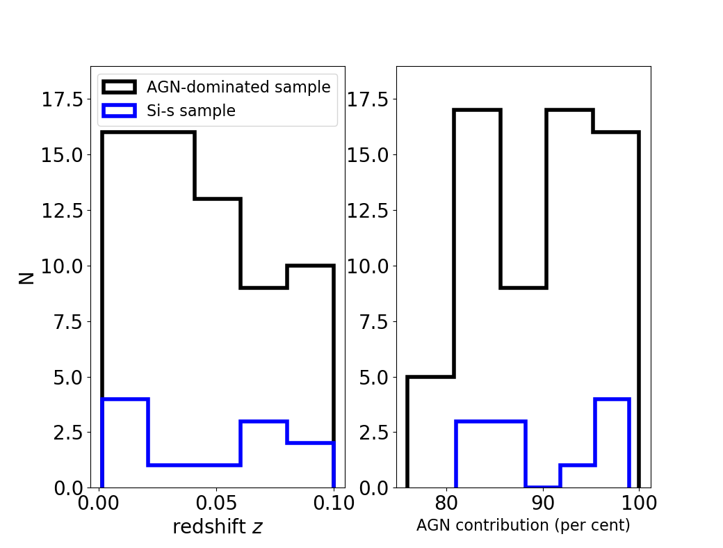
We use the latest version of the AGN catalog of Véron-Cetty & Véron 2010 and the sample of low luminosity type 1 AGN in Mason et al. 2012 to select AGN that have redshifts and available 2D low-resolution IRS/Spitzer spectra in the CASSIS database (Lebouteiller et al. 2011, v6.,). We select those objects with spectra extracted as point-sources that cover the m spectral range. The first criterion allows us to probe the MIR emission from the central region of the AGN, and the second one allows us to study both the 10 and 18m silicate features. As an exception, we include NGC 3998, a strong silicate emitter (Mason et al. 2012, e.g.,), which has a low-resolution spectrum in the 7.5-14.5m range and a high-resolution spectrum in the 14-35m range. In order to ensure that the emission in the IRS/Spitzer spectra is mostly dominated by dust heated by the AGN, we decompose them into their stellar, ISM and AGN emission (dust heated by AGN) components at m, using the spectral decomposition tool DeblendIRS (Hernán-Caballero et al. 2015). For more details on the spectral decomposition we refer the reader to Appendix A. We select only those objects (67) for which the spectral contribution due to AGN is (see Figure 1). Hereafter, we refer to the spectra of these objects as the AGN-dominated IRS/Spitzer spectra. Note that we refer here to the original spectra, not to the component obtained from the decomposition.
II.2 The IRS/Spitzer spectra
We obtained the reduced low resolution () IRS/Spitzer spectra from the CASSIS database (Lebouteiller et al. 2011, v6.,). The spectra include the SL1 (m) and SL2 (m) modules with a slit-width of 3.6 arcsec, and the LL1 (m) and LL2 (m) modules with a slit-width of 10.5 arcsec (Werner et al. 2004; Houck et al. 2004). We use the final stitched spectra between m. The different module spectra were stitched by scaling the LL and SL1 flux modules to the shortest module SL2 flux.
II.3 Measuring the silicate emission features
To measure the silicate emission features we start by interpolating a local continuum between both sides of the emission line complexes. We inspect each spectrum visually and choose three bands in which to measure the continuum. Band 1 is located at the blue extreme of the 10m silicate feature, while band 3 is located at the red extreme of the 18m silicate feature, and band 2 is located between the two silicates features. Band 1, 2 , and 3 are located within the , and m ranges.
In order to better define uncertainties in the continuum definition, which might be affected by the presence of Polycyclic Aromatic Hydrocarbon (PAH) molecular emission lines around 7m, and in some cases by the artificial ‘‘teardrop’’11 1 An excess of emission present in the 2D SL1 spectrum of some objects. feature around 14m, we trace fiducial mean values of each continuum band by bootstrapping on the measured fluxes (hatched pink regions in Figure 2). We generate 100 continuum values, considering the uncertainties, between band 1 and 2, and between band 2 and 3. We randomly associate shorter and longer wavelength mean continuum values to generate linear continua below the silicate features. We note that fitting a spline continuum gives similar results. The dark blue solid lines in Figure 2 are bootstrapped local continua derived from the continuum bands and they define the regions where we measure the strength of the silicate features.
Considering that the peak of the silicate features vary from object to object, we choose to measure the strength of the features at the wavelengths where they peak. However, for simplicity we still call them the 10 and 18m silicate features. The silicate strength is, hence, defined as the silicate peak relative to the continuum, at the wavelength where the silicate feature peaks (Hao et al. 2007, see e.g.,), according to the equation:
| (1) |
In Table 1 we list the mean and the 68 percent intervals for the objects with the largest silicate feature strengths. In Appendix B (Table 4) we list the silicate emission strengths for the full sample. On average, we find that type 1 AGN have a 10m silicate strength that peaks at m, and a 18m silicate strength that peaks at 17.3m.

| Name | Activitya | z | Ref. | Si | Si | |||
|---|---|---|---|---|---|---|---|---|
| erg s-1 | (m) | (m) | ||||||
| NGC7213 | LINER | 0.0058 | 42.2 | 6 | ||||
| PG2304+042 | Sy1.2 | 0.0420 | 43.4∗ | 9 | ||||
| PKS0518-45 | LINER | 0.0420 | 44.9 | 8 | ||||
| PG0844+349 | Sy1/QSO | 0.0640 | 43.7 | 1 | ||||
| PG1351+640 | Sy1.5/QSO | 0.0882 | 43.1 | 6 | ||||
| PG2214+139 | Sy1.0/QSO | 0.0658 | 43.8 | 1 | ||||
| PG0804+761 | Sy1/QSO | 0.1000 | 44.5 | 1 | ||||
| OQ208 | Sy1.5 | 0.0766 | 40.8 | 3 | ||||
| NGC4258 | LINERb | 0.0015 | 40.9 | 5 | ||||
| NGC3998 | LINER | 0.0035 | 41.2 | 4 |
Note.-∗This value needs to be used carefully, since we are using the high angular resolution spectrum to fix the band 3 and measure the m silicate feature strength. References:aNED and Véron-Cetty & Véron 2010, bMason et al. 2012. ∗Estimated from (15-150)+keV X-ray luminosity assuming a spectral power law with an index . References for hard X-ray luminosity: 1: Zhou & Zhang 2010; 2: Sambruna et al. 2011; 3: Ueda et al. 2005; 4: Younes et al. 2011; 5: Cappi et al. 2006; 6: Bianchi et al. 2009; 7:Brightman & Nandra 2011; 8: Winter et al. 2012; 9: Tueller et al. 2010; 10: Cusumano et al. 2010.

In most cases, our measurements, which were performed using the AGN-dominated Spitzer spectra, produce similar results to previous works (Hao et al. 2005; Thompson et al. 2009; Sirocky et al. 2008; Mendoza-Castrejón et al. 2015) (see Tables 4). Additionally, we compare our measurements of the silicate strengths with the values obtained using deblendIRS and find that they are similar within the uncertainties (see Figure 13 in Appendix A).
| Model name | Geometry | Dust composition | Scattering and absorption | Grain sizes∗(m) | |
|---|---|---|---|---|---|
| coefficients | Graphites | Silicates | |||
| Fritz06 | Smooth torus | Graphite and Silicates | graphite and silicates | 0.005-0.25 | 0.025-0.25 |
| Laor & Draine 1993 | |||||
| Nenkova08 | Clumpy torus | Standard ISM | graphites, Draine 2003 | (0.005-0.01)-0.25 | |
| silicates, Ossenkopf et al. 1992 | |||||
| Hoenig10 | Clumpy torus | Standard ISM | graphites, Draine 2003 | (0.005-0.01)-0.25 | |
| +standard ISM with large grains | silicates, Draine 2003 | 0.1-1.0 | |||
| +graphite dominated dust | Ossenkopf et al. 1992 | 0.05-0.25 | |||
| ( graphite and silicates) | |||||
| Hoenig17 | Disk+Outflow | Standard ISM | like Hoenig10 | (0.005-0.01)-0.25 | |
| +standard ISM with large grains | |||||
| Stalevski16 | Two phase media torus | Graphite and Silicates | Laor & Draine 1993 | 0.005-0.25 | 0.005-0.25 |
| Li & Draine 2001 | |||||
Note. The standard ISM is composed by of graphite and silicates. ∗Assuming MNR distribution (Mathis et al. 1977). The numbers inside the parenthesis indicate the minimal range of sizes for the smaller grains.
II.4 Sample selection
We build our final sample by selecting only those objects that show the strongest silicate emission features (see Table 1). From the original sample of 67 local type 1 AGNs we select those objects with the largest 10m silicate strength (, see Figure 3). The final sample is composed of 10 objects: six Seyfert (Sy) galaxies, and four low-ionization nuclear emission-line region (LINER) galaxies. Four of the Seyfert galaxies are also classified as PG QSOs. Note that we are not selecting the sample according to the type of AGN. We list the type only to give information about their basic properties.
Hereafter, we will refer to this sample as the type 1 AGN strong Silicate selected sample (Si-s). The sample spans a range of hard (2-10 keV) X-ray unobscured luminosities between erg s-1 and erg s-1.
III Dusty torus models

There are two types of torus models widely used in the literature: smooth torus models and clumpy torus models. Smooth models assume a continuous distribution of the dust in the torus (Pier & Krolik 1992; Granato et al. 1997; Efstathiou & Rowan-Robinson 1995; Fritz et al. 2006), while clumpy models assume a distribution of dusty clouds or clumps in a toroidal structure (Dullemond & van Bemmel 2005; Nenkova et al. 2008a; Nenkova et al. 2008b; Hönig & Kishimoto 2010b; Hönig & Kishimoto 2017).
For simplicity, smooth models assumed a continuous distribution of the dust in the torus, so the temperature of the dust decreases monotonically with the distance from the central BH. According to this type of model only type 1 AGN produce m silicate features in emission and type 2 AGN produce silicate features in absorption, implying an edge-on orientation with respect to the observer. In type 2 AGN, therefore, the outer region of the torus hides the emission produced by the hotter and warmer dust in the inner part of the torus. However, the silicate depth that this model predicts is larger than observed in type 2s, and it fails to explain silicate features in emission in type 2 QSOs (Sturm et al. 2006, e.g.,).
Conversely, clumpy models (Nenkova et al. 2008a; Nenkova et al. 2008b, e.g.,) never produce very deep absorption silicate features, and they predict silicate features in emission in type 1 and type 2 AGN for a large combination of parameters (Nikutta et al. 2009, see e.g.,). A third type of model combines clumpy and smooth properties to produce a two-phase medium dusty torus model (Stalevski et al. 2012; Stalevski et al. 2016). This model assumes a distribution of dusty clumps with constant and high density, embedded in a smooth dusty component of low density.
It was motivated by observational evidence that suggests that dust around AGN seems to have a multiphase filamentary structure (Wada et al. 2009; Wada 2012).
A more recent model proposes a geometry composed by a compact and geometrically thin disk in the equatorial region plus an extended elongated polar structure of clumpy dust, that is cospatial with the outflow of the AGN (Hönig & Kishimoto 2017). This geometry is inferred from interferometric observations of nearby Seyfert galaxies, where the bulk of the MIR emission originates from the polar region rather than the equatorial plane (Raban et al. 2009; Hönig et al. 2012; Hönig et al. 2013; Tristram et al. 2014; López-Gonzaga, & Jaffe 2016, e.g.,).
In this paper, we use the AGN-dominated IRS/Spitzer spectra of our Si-s sample of type 1 AGN to investigate which models are able to better reproduce the peak and shape of the strongest silicate emission features observed. In the following subsections we briefly describe the main geometrical and physical properties of the models and Table 2 summarizes the different geometries and dust compositions assumed for each model.
III.1 Smooth torus model of Fritz et al. 2006
This model is represented by a flared disc delimited by the inner and outer torus radius (Efstathiou & Rowan-Robinson 1995, e.g.,). The inner radius () is defined by the sublimation temperature of dust grains (1500 K) under the strong radiation produced by the central engine. The size of the torus is determined by the outer radius (, where is a free parameter), and the angular width of the torus (see the cartoon (a) in Figure 4). This model assumes that the dust is composed of graphite grains (53 per cent) with sizes from 0.005 to 0.25m, and silicate grains (47 per cent) with sizes from 0.025 to 0.25m. The grain sizes are distributed according to Mathis et al. 1977. For the two species they used the scattering and absorption coefficients given by Laor & Draine 1993. The dust is illuminated by an isotropic central point-like emitting source, which is represented by a broken power law of the form , with if m, if m, and if m. Other parameters of the model are the viewing angle , the polar () and radial () indices of the gas density distribution within the torus, and the optical depth . For a more complete description of this model see Fritz et al. 2006.
III.2 Clumpy torus models of Nenkova et al. 2008a; Nenkova et al. 2008b
This type of model assumes a central point-like emitting source surrounded by a toroidal distribution of clouds. The emission of the central source is characterized by a broken power law of the form for m, for , for m, and a constant power-law between 0.01 and 0.1m. Due to its clumpy nature, the central source can directly heat the dust in the inner region of the torus and the dust located at several sublimation radii from the central source. This model assumes standard Galactic spherical dust grains (standard ISM) composed of graphites (Draine 2003, ,) and silicates (Ossenkopf et al. 1992, ,), with a power-law distribution of grain sizes (), where m and m, respectively. This model has six free parameters: the viewing angle , the number of clouds along the equatorial ray , the angular width , the radial extend , the index of the radial distribution of clouds , and the optical depth per cloud (see cartoon (b) in Figure 4). For a more complete description of this model see Nenkova et al. 2008a; Nenkova et al. 2008b.
III.3 Clumpy torus models of Hönig & Kishimoto 2010b
In this case the toroidal distribution of dusty clumps surrounds a central point-like emitting source, that is described by a broken power-law of the form for m, for m, constant for between 0.03m and m, and for between 0.3 and 3m. They modeled the torus following a 3D Monte Carlo radiative transfer simulation. These kinds of simulations fail to properly sample optically thick surface regions with enough grid cells so that each cell is optically thin, which results in underestimating the emission temperature and resulting in a smaller number of model clouds with respect to Nenkova et al. 2008a; Nenkova et al. 2008b. The dust is composed of three components: a standard ISM component, a standard ISM component with larger grains (m and m), and intermediate to larger grains (m and m) with graphite and silicates. The free parameters that describe this model are the viewing angle , the number of clouds along the equatorial ray , the half-opening angle , the index of the radial distribution , and the optical depth (see cartoon (b) in Figure 4). For a more complete description of this model see Hönig & Kishimoto 2010b.
III.4 Clumpy disk+outflow models of Hönig & Kishimoto 2017
This type of model is based on the parametrization of the clumpy torus model of Hönig & Kishimoto 2010b, but instead of adding a blackbody component to take into account the NIR emission, they include a set of different sublimation temperatures for silicate and graphite dust that results in more emission from graphite located in the inner edge of the torus. In this way, when the dust is heated to temperatures K smaller silicate grains are destroyed leaving only graphite grains that can be heated up to 1900 K. In the innermost radius only, grains with a size between 0.075 and 1m survive.
The clouds are distributed according to a radial power-law , where is the power law index and the distance from the black hole in units of the sublimation radius . They also add a polar outflow, modeled as a hollow cone that can be characterized by the radial distribution of dust clouds in the wind , the half-opening angle of the wind (), and the angular width (). Other parameters are the number of clouds along the equatorial ray , and the scale height in the vertical Gaussian distribution of clouds in the disk, (see cartoon (c) in Figure 4). For a more complete description of this model see Hönig & Kishimoto 2017.
III.5 Two-phase medium dusty torus models of Stalevski et al. 2016
This kind of models assumes a distribution of high density dusty clumps embedded in a low density smooth dusty component. This assumption produces both weaker silicate features and a pronounced NIR emission. They assume that the accretion disk in the nucleus radiates as a broken power-law of the form , where for a spectral range of m, for m, for m, and for m. The dust is distributed following a law that allows a density gradient along the radial () and polar () directions, inside a flare disc defined by the inner (), outer radii () and half opening angle. The inner radius is defined by the sublimation temperature of 1500 K for an average dust grain size of 0.05 m. They assumed a standard ISM dust composition with optical properties from Laor & Draine 1993 and, Li & Draine 2001. For a more complete description of this model see Stalevski et al. 2012; Stalevski et al. 2016.


IV Analysis
IV.1 Synthetic and observed silicate peak wavelengths and strengths
In this section we explore how well the dusty torus models reproduce the central wavelength and strength of both 10 and 18m silicate features, and the NIR () and MIR () spectral indexes. In order to make a proper comparison the synthetic and observed central wavelength and strength of both the 10 and 18m silicate features are measured following the same methodology described in Section 2.3, and fixing the bands to the sides of the silicate features between 7-7.5m, 14-15m, and m. The synthetic and observed spectral indexes and are measured between 5.5-7.5m, and between 7.5-14.0m, respectively, according to the following definition , with (Buchanan et al. 2006, see e.g.,).
In Figures 5 and 6 we plot the wavelength of the peak of the both 10 and 18m silicate features and the strengths of both silicate features as predicted by the models, and as observed in the AGN-dominated IRS/Spitzer spectra of the Si-s sample. Additionally, we color-coded the objects according to their bolometric luminosity, which we estimate using the hard X-ray luminosity and the relation derived by Marconi et al. 2004 and Alexander, & Hickox 2012.
Since the models are probabilistic in nature, we compare the envelope of measurements performed on the models to the measurements of the Si-s AGN sample. While the Fritz 06, Stalev16 and Nenkova08 models envelope covers the wavelength space (Figure 5) where our Si-s AGN measurements lie, the Hoenig10 and Hoenig17 models leave miss one and two objects, respectively, with the lowest value central wavelength of the 18m silicate feature. Curiously, these objects are of low bolometric luminosity (OQ 208 and NGC 4258).
For the silicate strengths (Figure 6) we note that the range of synthetic values sampled by the models mostly match the observations. However, we also note that Hoenig10 and Hoenig17 models show a narrower range of values respect to the other models. Additionally, the Hoenig17 model never predicts both silicates in absorption. Similar results were reported for a larger sample of AGN (González-Martín et al. 2019b). Finally, all the models tend to produce extremely prominent silicate emission features that have not been observed.
In Figure 7 we compare the synthetic and observed silicate strength of the 10m silicate feature with the and spectral indexes. We note that the range of synthetic values sampled by the Fritz06, Hoenig10, and Hoenig17 models mostly match the observations, independently of the bolometric luminosity. However, the Nenkova08 and Stalev16 models miss several of the NIR and MIR spectral indexes observed. Note that NGC 3998 is excluded from plots in Figures 5, 6 and 7 because the short spectral range (m) cover by the low resolution IRS/Spitzer spectrum of this object.

IV.2 Modeling
We apply the torus models using the computational spectral fitting tool XSPEC, which is part of the HEASOFT22 2 https://heasarc.gsfc.nasa.gov software. These models were recently converted into the XSPEC format in order to fit data in a similar way (González-Martín et al. 2019a, see section 2 in). We also use the set of synthetic stellar and empirical HII components (ISM) previously converted into XSPEC format (González-Martín et al. 2019a). The former corresponds to a stellar population of 1010 years and solar metallicity from the stellar spectral libraries of Bruzual & Charlot 2003, while the empirical HII components are average starburst templates from Smith et al. 2007.
We model the AGN-dominated IRS/Spitzer spectrum of each object in the Si-s sample, using each one of the four torus family models and the disk+outflow models. Additionally, we add a stellar synthetic and/or HII empirical component to investigate in which cases adding one or both components really improves the fitting. We also add foreground extinction to the torus models by using the ZDUST component (Pei 1992).
In detail, we start converting the IRS/Spitzer spectra into the XSPEC format, loading the data into XSPEC, removing the parts of the spectra dominated by emission lines, and modeling the spectra assuming the following component combinations:
- •
1: AGN dust emission: torus models or disk+outflow model
- •
2: AGN + stellar
- •
3: AGN + HII
- •
4: AGN + stellar + HII
For each step, we save the reduced , the parameters of the model with their uncertainties, and the emission contribution of each component to the total emission of the IRS/Spitzer spectrum between 5.5 to 30 m. In those cases where we reported the case as “non-modeled”. We perform this procedure for each torus model, resulting in 20 spectral fits per object. Figure 8 shows, for each torus model, the number of spectral fits obtained, using one, two, or three components. Those cases in which none of the component combinations (1,2,3, or 4) are able to model the spectrum with a are called “non-modeled” spectral fits (see Table 5 in Appendix C). In the next section we investigate which model best fits the peak and strength of both silicate emission features in the Si-s sample.

IV.3 Model comparison
In most cases, we find that the same object can be modeled assuming one (AGN), two (AGN+stellar or AGN+HII), or three components (AGN+Stellar+HII) with a . For each object and torus model we use the statistical f-test, which allows us to evaluate in which cases the addition of a new component improves the fit from a statistical point of view. We add a new component when the f-test probability is . The computational tool xspec includes the ftest command line, which allows us to calculate the f-statistic and its probability, when new and old values of and the degrees of freedom (dof) are provided. As an example, in Figure 9 we show the best fit of the IRS/Spitzer spectrum of PG 0844+349 for each torus model. For this particular object the Fritz06, Nenkova08, and Stalev16 models need an additional stellar component to fit the spectrum, while the Hoenig10 and Hoenig17 models need also the HII component. Additionally, for this object, we observe that clumpy and disk+outflow models produce the flattest residuals within the uncertainties and smaller (see bottom panel in Figure 9 and Table 3).

| Component contributions | Component contributions | ||||||||||
| Name | Best combination | AGN | Stellar | HII | Name | Best combination | AGN | Stellar | HII | ||
| () | () | () | () | () | () | ||||||
| Smooth torus models of Fritz et al. 2006 | Disk+outflow models of Hönig & Kishimoto 2017 | ||||||||||
| PG2304+042 | 1.92 | Torus+Stellar | 93 | 7 | 0 | PG2304+042 | 0.57 | Disk+outflow+Stellar | 93 | 7 | 0 |
| PG 0844+349 | 1.20 | Torus+Stellar | 93 | 7 | 0 | PKS0518-45 | 0.31 | Disk+outflow | 100 | 0 | 0 |
| PG 1351+640 | 1.52 | Torus+Stellar | 97 | 3 | 0 | PG 0844+349 | 0.13 | Disk+outflow+Stellar+HII | 87 | 5 | 8 |
| PG 2214+139 | 1.52 | Torus+Stellar | 96 | 4 | 0 | PG 2214+139 | 0.20 | Disk+outflow+Stellar+HII | 95 | 1 | 4 |
| PG 0804+761 | 0.63 | Torus+Stellar | 94 | 6 | 0 | PG 0804+761 | 0.49 | Disk+outflow+HII | 95 | 0 | 5 |
| NGC 3998 | 1.91 | Torus+Stellar | 100 | 0 | 0 | OQ 208 | 1.78 | Disk+outflow+Stellar | 98 | 2 | 0 |
| NGC 4258 | 1.88 | Disk+outflow+HII | 62 | 0 | 38 | ||||||
| . | . | . | . | . | NGC 3998 | 0.39 | Disk+outflow | 100 | 0 | 0 | |
| Clumpy torus models of Nenkova et al. 2008a; Nenkova et al. 2008b | Two-phase media torus models of Stalevski et al. 2016 | ||||||||||
| NGC7213 | 1.11 | Torus+Stellar | 96 | 4 | 0 | PG2304+042 | 1.99 | Torus+Stellar | 93 | 7 | 0 |
| PG2304+042 | 1.25 | Torus+Stellar | 92 | 8 | 0 | PKS0518-45 | 1.65 | Torus | 100 | 0 | 0 |
| PKS0518-45 | 1.29 | Torus+Stellar | 97 | 3 | 0 | PG 0844+349 | 0.81 | Torus+Stellar | 92 | 8 | 0 |
| PG 0844+349 | 0.32 | Torus+Stellar | 91 | 9 | 0 | PG 2214+139 | 0.91 | Torus+Stellar+HII | 82 | 10 | 8 |
| PG 1351+640 | 1.92 | Torus+Stellar | 99 | 1 | 0 | PG 0804+761 | 1.11 | Torus+Stellar | 90 | 10 | 0 |
| PG 2214+139 | 1.92 | Torus+Stellar | 87 | 13 | 0 | ||||||
| PG 0804+761 | 1.60 | Torus+Stellar | 89 | 11 | 0 | . | . | . | . | . | . |
| OQ 208 | 0.32 | Torus+Stellar+HII | 91 | 3 | 6 | . | . | . | . | . | . |
| NGC 4258 | 0.78 | Torus+Stellar+HII | 66 | 4 | 30 | . | . | . | . | . | . |
| NGC 3998 | 0.32 | Torus+Stellar | 81 | 19 | 0 | . | . | . | . | . | . |
| Clumpy torus models of Hönig & Kishimoto 2010b | . | . | . | . | . | . | |||||
| PG2304+042 | 1.18 | Torus | 100 | 0 | 0 | . | . | . | . | . | . |
| PKS0518-45 | 0.46 | Torus+Stellar+HII | 89 | 6 | 5 | . | . | . | . | . | . |
| PG 0844+349 | 0.20 | Torus+Stellar+HII | 80 | 10 | 10 | . | . | . | . | . | . |
| PG 2214+139 | 0.71 | Torus+Stellar+HII | 76 | 9 | 14 | . | . | . | . | . | . |
| PG 0804+761 | 1.79 | Torus+Stellar+HII | 76 | 9 | 15 | . | . | . | . | . | . |
| NGC 4258 | 1.64 | Torus+Stellar+HII | 67 | 3 | 29 | . | . | . | . | . | . |
| NGC 3998 | 0.40 | Torus | 100 | 0 | 0 | . | . | . | . | . | . |
In Figure 10 we plot the histogram of the fractional contribution of each spectral component. The AGN component dominates the emission in all cases, which is expected due to our selection of AGN-dominated IRS/Spitzer spectrum sources.
Fritz06 models are able to reproduce the IRS/Spitzer spectra in seven of 10 objects. The AGN component contributes more than . The Nenkova08 models reproduce the IRS/Spitzer spectra of 10 objects, in most cases with an AGN contribution , except for NGC4258 for which the AGN component contributes . For Hoenig10 models we find that four of the objects can be modeled with an AGN contribution , and three other (PG2214+139, PG0804+761, and NGC4258) with a contribution between 67 and 76 . The Hoenig17 models are able to fit seven of the objects with an AGN contribution , and NGC 4258 with an AGN component that contributes . Finally, in the case of two-phase medium models of Stalevski et al. 2016 only five of the 10 objects can be reproduced with a contribution of the AGN .
Irrespective of the model used, NGC4258 always need a large () contribution from the HII component. It is possible that in this case the spectral decomposition tool DeblendIRS is not perfectly separating the different spectral contributions at MIR. We also note that in all cases the stellar component is necessary to take into account the emission in the bluer extreme of the spectrum, while the HII component is necessary to take into account the emission in the redder extreme of the spectrum. A similar result was also found by González-Martín et al. 2019a for a large sample of AGN.
We obtain upper (or lower) limits of the resulting free parameters and covering factors. The covering factor is defined as , where is the probability that a photon emitted in the central engine is able to escape without being absorbed by the torus (in the case of the smooth torus and two-phase medium torus models) or by a dusty cloud in clumpy torus models (Nenkova08, Hoenig10). In the case of Hoenig17 models, the covering factor derived is the sum of the geometrical covering factors of the disk and the covering factor of the outflow (González-Martín et al. 2019b, see).
To obtain well constrained parameters a detailed modeling that includes NIR and far-infrared (FIR) data is necessary (Ramos Almeida et al. 2014, see e.g.,). However, modeling simultaneously the NIR and MIR components of the IRS/Spitzer spectrum of type 1 AGNs has been a challenge (Mor et al. 2009; Martínez-Paredes et al. 2017; Hernán-Caballero et al. 2015, e.g,). In this work we assume the NIR as a stellar component. Our purpose is to show if any of the proposed models are able to explain both the peak and shape of the strongest silicate emission features. For this purpose, we only need to check that the range of values of the covering factors obtained from modeling the IRS/Spitzer spectra with each model are within the range of values expected for type 1 AGNs (Ramos Almeida et al. 2011; Alonso-Herrero et al. 2011; Ichikawa et al. 2015; Mateos et al. 2016; Martínez-Paredes et al. 2017; González-Martín et al. 2017, see e.g.,).
We note that on average the smooth models produce a dusty torus with a small angular widths, with low and high viewing angles, although the angular width is poorly constrained. The dusty clumpy torus models of Nenkova08 produce both large and low viewing angles and a range of angular width from low (15 degrees) to high (70 degrees) values, and a number of clouds along the equatorial ray that are in general clouds, resulting in escape probabilities . The clumpy models of Hoenig10 produce values of the viewing angle that range from nearly 30 to 80 degrees, angular widths around 55 degrees, and number of clouds in the range 2.5 to 10.0. The viewing angles in disk+outflow models of Hoenig17 that we find is between 0 and 50 degrees and the angular widths between 30 and 45 degrees. Although in three cases we obtain lower limits of the angular width, indicating that this could be larger. The two-phase models of Stalev16 produce on average large viewing angles (), only in one case we obtain a viewing angle around 10 degrees, and the angular width is around 80 degrees, resulting in very obscured AGNs (see Tables 6,7,8, 9, and Figure 17 in Appendix C).
In general, Fritz06 and Hoenig17 models produce lower covering factors than Nenkova08, Hoenig10 and Stalevski16 models. Fritz06 and Hoenig17 models produce covering factors around 0.2, although they range from 0 to 1. The Nenkova08 model produces covering factors around 0.6 with a range from 0.3 to 1.0. These values are consistent with the range of values obtained by Martínez-Paredes et al. 2017 for a sample of PG QSOs using Nenkova08 models. Feltre et al. 2012 compare smooth and clumpy torus models of Nenkova08 and found that both torus model families produce similar MIR continuum shapes for different model parameters. In the Hoenig10, and Stalevski16 models the covering factors are large (around 0.8), probably due the fact that in these models the angular width of the torus tends to be larger, which leads to a more obscured AGN.
IV.4 Residuals
Using the spectral residuals for all modeled and non-modeled cases we calculate the average spectral residuals for each torus model. The vertical black solid lines in Figure 11 represents the mean wavelength where the silicate features peak in the IRS/Spitzer spectra, and the black dotted lines their intervals.
In order to discuss qualitatively the similarities and differences between the residuals of the models we divide the spectral range into three parts in Figure 11. These parts are the region bluewards of 10m, between m and m, and redwards 18m. In part (a) we observe that on average, around 5m, Fritz06, Nenkova08, Hoenig10, Stalev16 models are the worst at reproducing the bluer extreme of the spectra within the uncertainties. However, at longer wavelengths the Fritz06 and Stalevski16 models are the least accurate at reproducing the shape of the spectra. The Hoenig17 models best reproduce the spectra at all wavelengths within the uncertainties. In the part (b) Nenkova08 show the flattest residual, while in the redder extreme the Fritz06 and Stalevski16 models show the largest residuals, while the Hoenig10 and Hoenig17 models shows flatter residuals. In part (c) all models show similar residuals, although Nenkova08 show the flattest residual within the uncertainties.
We also observe that the Fritz06 and Stalevski16 models underestimate the strength of the 10 and 18m silicate features, while the Nenkova08, Hoenig10, and Hoenig17 models best reproduce the peak and the shape of both features. In general we note that Hoenig17 and Nenkova08 models show flatter residuals, resulting in the models that best reproduces the shape and the peak of the strong silicate features observed in these objects.
Some objects deserve particular attention. For instance, in Figure 19 we can see that for NGC 7213 we require the stellar component to fit the bluer extreme of the spectrum, but that both silicate peaks are still underestimated by the Nenkova08 models.
PG 1351+640 is modeled only by the smooth and clumpy models of Nenkova08. In both cases it is necessary to add the stellar component, which contributes and in the case of smooth (Fritz06) and clumpy models (Nenkova08 and Hoenig10), respectively. OQ208 is modeled only by the Nenkova08 and Hoenig17 models. In this case the residuals from the Nenkova08 model are flatter than the residuals from the Hoenig17 models, although in the case of the Nenkova08 model it is necessary to include the HII component with a contribution of , in addition to the stellar component () in order to fit the redder extreme of the spectrum. In contrast, the Hoenig17 model is able to reproduce the entire spectral range requiring only a small contribution from the stellar component (). The remaining objects are modeled successfully by the Nenkova08, Hoenig10, and Hoenig17 models.


We divide the objects in the Si-s sample into three groups according to their bolometric luminosities and BH accretion rates. For each group and torus model we combine the residual obtained from fitting the AGN-dominated Spitzer spectrum with the components C1 (AGN), C2 (AGN+Stellar), C3 (AGN+HII), and C4 (AGN+Stellar+HII). In Figure 12 we plot the average residual for each group. We note that for the first group, all models are unable to produce a flat residual around the 10m silicate feature. But, for the second group, which covers a larger range of bolometric luminosities and BH accretion rates, all the residuals become flatter. At the largest bolometric luminosites of the third group all models show the flattest residuals. These results show that all models fail in reproduce the central wavelength of the 10m silicate feature in the objects with lower bolometric luminosities, as we see in Figure 5 in Section 4.1. Additionally, we note that the Hoenig17 models always produce the flattest residual around 5m for low, intermediate, and high luminosities.
V Discussion
In the previous section we used four different torus models (smooth, clumpy, two-phase medium, and disk+outflow) to reproduce the strongest silicate features observed in type 1 AGNs. These features appear broader and shifted with respect to the silicate emission features observed in the standard ISM, suggesting a different dust composition (or geometry) of the torus or surrounding dust of AGNs. We discuss below the dust distribution (Section 5.1) and composition (Section 5.2) of the dust. We also discuss the deficiencies of the models to reproduce the strong silicate emission features in Section 5.3.
V.1 Dust distribution
Based on our analysis the clumpy models of Nenkova08 (), Hoenig10 (), and Hoenig17 () produce a better fitting of the IRS/Spitzer spectra than the smooth () and two-phase medium () models. This result is in agreement with the previous evidence that the surrounding medium around the AGN should be clumpy (see Ramos Almeida, & Ricci 2017, and references therein). Indeed, Mendoza-Castrejón et al. 2015 found that isolated type 1 AGN have a clumpy dust distribution, while interacting type 1 AGN can have both clumpy or smooth dusty distributions. Additionally, we find that all models produces flatter residual in high luminosity AGN than in low luminosity AGN, probably due to all models better sample the central wavelength and both 10 and 18m silicate features of high luminosity AGNs. However, a high luminosities Hoenig17 models produce the flattest residual along all the spectral range.
Mor et al. 2009 used IRS/Spitzer spectra of a sample of 26 nearby QSOs to constrain the clumpy models of Nenkova08. They argue that in order to model the entire spectral range between 5-30m they need to add two more components, one that takes into account the emission produced by the dust in the narrow line region (NLR) (Schweitzer et al. 2008), and another one that takes into account the emission produced by dust close to the AGN, not directly related with the dusty torus (Minezaki, et al. 2004; Riffel et al. 2009; Kishimoto et al. 2007, e.g.,). However, Alonso-Herrero et al. 2011 showed, for a sample of local Seyferts, that when high angular resolution data at NIR and MIR is used, it is not necessary to add any additional components in order to constrain the clumpy models of Nenkova08, although for some type 1 Seyferts galaxies they found that the NIR emission is underpredicted by the fitted SED. In a previous work, we used the starburst-subtracted IRS/Spitzer spectra from m plus NIR high angular resolution data from the Near Infrared Camera and Multi-Object Spectrometer (NICMOS) on HST for a sample of 20 nearby QSOs in order to constrain the clumpy torus models of Nenkova08. Martínez-Paredes et al. 2017 found that including the spectral range between m resulted in a poor fitting of the 10m silicate emission feature. In this work we find that the AGN-dominated Spitzer spectra of the Si-s type 1 AGN can be fitted by Nenkova08 and/or Hoenig10 models by adding a stellar component that takes into account the bluer spectral range, and in some cases the HII component, in order to improve the fitting in the redder spectral range. A similar result was also found for a large sample of AGNs (González-Martín et al. 2019a; González-Martín et al. 2019b).
Hernán-Caballero et al. 2017 found, for a sample of 85 QSOs, that a superposition of two blackbodies between 1.7-8.4m, with temperatures around 1000 K for the hot blackbody component, and 400 K for the warm blackbody component, can fit the Spitzer spectra between 0.1 and 10m. They argue that an additional hotter component of dust is necessary to reproduce the excess emission at 1-2m. On the other hand, Lyu et al. 2017 argues that the strong silicate emission features observed in dust-deficient PG QSOs can be explained assuming a reduced height scale of the warm dust, i.e., the dust between the sublimation zone and the outer region of cold dust, allowing for less interception of the radiation from the accretion disk with the inner dust, resulting in a decrease of the MIR continuum, but keeping the heating of the outer dust responsible for the silicate emission features invariant (Lyu et al. 2017, see Figure 20 in).
V.2 Dust composition
In general, the Nenkova08 models produce a better fit than the Hoenig10 ones. They assume the same geometry, but the former uses a standard dust composition, while the latter includes standard ISM dust plus standard ISM with large grains, and also a composition of dust mostly dominated by graphite. The Hoenig10 models assume this dust composition in order to take into account the observational suggestion that the dust composition in AGN deviates from standard ISM dust (Suganuma et al. 2006; Kishimoto et al. 2007). One of the clear improvements in the Hoenig17 models is that they allow the existence of different dust compositions in different parts of the surrounding dusty structure (disk+outflow).
The chemical composition of the dust has been largely studied for the ISM (see Henning 2010, and references therein), and to a lesser extent in AGN (see Lyu, Hao & Li 2014, and references therein). However, determining the exact chemical composition of the dust has been challenging. Srinivasan et al. 2017 studied the dust composition of a large sample of PG QSOs with a redshift , that showed the 10m silicate feature in emission. They found that the dust is mostly composed of amorphous oxides and silicates, plus a small fraction in crystalline form. However, this small fraction is nearly four times larger than the last upper limit () reported by Kemper et al. 2005 for the ISM, and more similar to the upper limit () previously reported by Li & Draine 2001 for the ISM.
V.3 Deficiencies of the models
In general we find that neither the peak nor the shape of the silicate features of the AGN-dominated IRS/Spitzer spectra of the Si-s type 1 AGN are perfectly reproduced by the models. However, we note that for each object either the Hoenig17 or the Nenkova08 models produce the smallest and flattest residuals. Hönig & Kishimoto 2017 point out that their dust composition explains both the observed small NIR reverberation mapping and interferometric sizes with dust sublimation physics. They argue that this combination of disk+outflow clumpy models is able to reproduce the m bump in type 1 AGN, and preserve the MIR bump produced by the wind. Indeed, according to this model a standard ISM composition of the dust in the wind would be the responsible for the emission of the silicate features. García-González et al. 2017 found that the Hoenig17 (disk+outflow) models predict MIR slopes (between m) and silicate strengths at 10 m that are in agreement with the values observed in type 1 AGN. Particularly, they noted that when clouds are more concentrated towards the inner region of the torus (Hönig & Kishimoto 2010b; Ramos Almeida et al. 2011; Ichikawa et al. 2015; Martínez-Paredes et al. 2017, see e.g.,), the MIR spectral indices are flatter and the silicate features are stronger than those observed in Seyferts and QSOs.
VI Summary and conclusions
In order to investigate which model better reproduces the shape and peak of the strongest 10m silicate emission features observed in type 1 AGN, we measure the 10m silicate emission strength for a sample of local () type 1 AGN, for which their IRS/Spitzer spectra is mostly dominated by the emission of non-stellar processes ().
We find that these objects show silicate features in emission. On average the 10m silicate feature has a strength of that peaks at 10.3m, and a 18m silicate strength of that peaks at m. We find that 10 objects are among the AGN with the largest 10m silicate strengths (, Si-s sample), and that some of them have been previously classified as objects with prominent silicate features.
We use four different torus models, Fritz06 (Fritz et al. 2006), Nenkova08 (Nenkova et al. 2008a; Nenkova et al. 2008b), Hoenig10 (Hönig & Kishimoto 2010b), Stalevski16 (Stalevski et al. 2016) and a disk+outflow (Hönig & Kishimoto 2017, Hoenig17,) model to fit the IRS/Spitzer spectra of the Si-s sample, and investigate which model better reproduces the peak and shape of both silicate emission features. The models assume different dust distributions, namely, smooth, clumpy, and a two-phase medium, as well as different dust compositions. We find that in most cases it is necessary to add a stellar or HII component in order to improve the fit. In most cases we find that the contribution of these components is , in agreement with our selection requirement that the spectra be dominated by the emission of the AGN. The exceptions is NGC 4258 for which the spectral decomposition seems to underestimate the HII component.
We find that in general Fritz06 and Hoenig17 models produce lower covering factors than the Nenkova08, Hoenig10, and Stalevski17 models. The values are consistent with those reported in previous works for type 1 AGN. We find that the individual and average spectra are reproduced better with clumpy torus models than smooth models. Moreover, the Hoenig17 model shows the flattest residuals along all the spectral range between m, while the rest of models fail to reproduce the bluer extreme of the spectrum. However, on average none of the models are able to exactly reproduce the peak and shape of the silicate features.
In the near future the Mid-Infrared Instrument (MIRI) onboard of the James Webb Space Telescope will provide high angular resolution with higher sensitivity and spectral resolution observations which will allow an in-depth investigation of the dust properties in active galaxies. Additionally, new models that include a better description of the properties of the dust will be required.
Acknowledgements
MM-P acknowledges support by the KASI and UNAM-DGAPA postdoctoral fellowships. This work is partially supported by the KASI project 2019184100 and Conacyt project CB-2016-281948. O.G.-M. acknowledges support by the PAPIIT projects IA100516. A.A.-H. acknowledges support through grant PGC2018-094671-B-I00 (MCIU/AEI/FEDER,UE). AAH’s work was done under project No. MDM-2017-0737 Unidad de Excelencia ”María de Maeztu”- Centro de Astrobiología (INTA-CSIC). YK acknowledges support from grant DGAPA-PAPIIT 106518, and from program DGAPA-PASPA. T.H acknowledges the support from the National Research Foundation of Korea (NRF) grant funded by the Korea government (MSIT) (2019R1A2C1087045). CRA acknowledges financial support from the Spanish Ministry of Science and Innovation (MICINN) through project PN AYA2013-47742- C4-2-P. CRA also acknowledges the Ramon y Cajal Program of the Spanish Ministry of Economy and Competitiveness. This work is based on observations obtained with the Spitzer Space Observatory, which is operated by JPL, Caltech, under NASA contract 1407. This research has made use of the NASA/IPAC Extragalactic Database (NED) which is operated by JPL, Caltech, under contract with the National Aeronautics and Space Administration. CASSIS is a product of the Infrared Science Center at Cornell University, supported by NASA and JPL.
References
- Antonucci (1993) Antonucci, R. 1993, ARA&A, 31, 473
- Alexander, & Hickox (2012) Alexander, D. M., & Hickox, R. C. 2012, New Astronomy Reviews, 56, 93
- Alonso-Herrero et al. (2011) Alonso-Herrero, A., Ramos Almeida, C., Mason, R., et al. 2011, ApJ, 736, 82
- Alonso-Herrero et al. (2016) Alonso-Herrero, A., Poulton, R., Roche, P. F., et al. 2016, MNRAS, 463, 2405
- Bianchi et al. (2009) Bianchi, S., Bonilla, N. F., Guainazzi, M., Matt, G., & Ponti, G. 2009, A&A, 501, 915
- Brightman & Nandra (2011) Brightman, M., & Nandra, K. 2011, MNRAS, 413, 1206
- Bruzual & Charlot (2003) Bruzual, G., & Charlot, S. 2003, MNRAS, 344, 1000
- Buchanan et al. (2006) Buchanan, C. L., Gallimore, J. F., O’Dea, C. P., et al. 2006, AJ, 132, 401
- Cappi et al. (2006) Cappi, M., Panessa, F., Bassani, L., et al. 2006, A&A, 446, 459
- Cusumano et al. (2010) Cusumano, G., La Parola, V., Segreto, A., et al. 2010, Astronomy and Astrophysics, 510, A48
- Draine (2003) Draine, B. T. 2003, ApJ, 598, 1026
- Draine et al. (2007) Draine, B. T., Dale, D. A., Bendo, G., et al. 2007, ApJ, 663, 866
- Dullemond & van Bemmel (2005) Dullemond, C. P., & van Bemmel, I. M. 2005, A&A, 436, 47
- Dudik et al. (2007) Dudik, R. P., Weingartner, J. C., Satyapal, S., et al. 2007, ApJ, 664, 71
- Efstathiou & Rowan-Robinson (1995) Efstathiou, A., & Rowan-Robinson, M. 1995, MNRAS, 273, 649
- Elvis et al. (1994) Elvis, M., Wilkes, B. J., McDowell, J. C., et al. 1994, ApJS, 95, 1
- Feltre et al. (2012) Feltre, A., Hatziminaoglou, E., Fritz, J., & Franceschini, A. 2012, MNRAS, 426, 120
- Fritz et al. (2006) Fritz, J., Franceschini, A., & Hatziminaoglou, E. 2006, MNRAS, 366, 767
- García-González et al. (2017) García-González, J., Alonso-Herrero, A., Hönig, S. F., et al. 2017, MNRAS, 470, 2578
- Granato et al. (1997) Granato, G. L., Danese, L., & Franceschini, A. 1997, Mem. Soc. Astron. Italiana, 68, 39
- González-Martín et al. (2013) González-Martín, O., Rodríguez-Espinosa, J. M., Díaz-Santos, T., et al. 2013, A&A, 553, A35
- González-Martín et al. (2017) González-Martín, O., Masegosa, J., Hernán-Caballero, A., et al. 2017, ApJ, 841, 37
- González-Martín et al. (2019a) González-Martín, O., Masegosa, J., García-Bernete, I., et al. 2019, arXiv e-prints, arXiv:1908.11381
- González-Martín et al. (2019b) González-Martín, O., Masegosa, J., García-Bernete, I., et al. 2019, arXiv e-prints, arXiv:1908.11389
- Hatziminaoglou et al. (2015) Hatziminaoglou, E., Hernán-Caballero, A., Feltre, A., et al. 2015, ApJ, 803, 110
- Hao et al. (2005) Hao, L., Spoon, H. W. W., Sloan, G. C., et al. 2005, ApJ, 625, L75
- Hao et al. (2007) Hao, L., Weedman, D. W., Spoon, H. W. W., et al. 2007, ApJ, 655, L77
- Hernán-Caballero et al. (2015) Hernán-Caballero, A., Alonso-Herrero, A., Hatziminaoglou, E., et al. 2015, ApJ, 803, 109
- Henning (2010) Henning, T. 2010, ARA&A, 48, 21
- Hernán-Caballero et al. (2017) Hernán-Caballero, A., Hatziminaoglou, E., Alonso-Herrero, A., et al. 2017, Frontiers in Astronomy and Space Sciences, 4, 30
- Hönig et al. (2010a) Hönig, S. F., Kishimoto, M., Gandhi, P., et al. 2010, A&A, 515, A23
- Hönig & Kishimoto (2010b) Hönig, S. F., & Kishimoto, M. 2010, A&A, 523, A27
- Hönig et al. (2012) Hönig, S. F., Kishimoto, M., Antonucci, R., et al. 2012, The Astrophysical Journal, 755, 149
- Hönig et al. (2013) Hönig, S. F., Kishimoto, M., Tristram, K. R. W., et al. 2013, The Astrophysical Journal, 771, 87
- Hönig & Kishimoto (2017) Hönig, S. F., & Kishimoto, M. 2017, ApJ, 838, L20
- Houck et al. (2004) Houck, J. R., Roellig, T. L., Van Cleve, J., et al. 2004, Proc. SPIE, 5487, 62
- Ichikawa et al. (2015) Ichikawa, K., Packham, C., Ramos Almeida, C., et al. 2015, ApJ, 803, 57
- Kemper et al. (2005) Kemper, F., Vriend, W. J., & Tielens, A. G. G. M. 2005, ApJ, 633, 534
- Kishimoto et al. (2007) Kishimoto, M., Hönig, S. F., Beckert, T., et al. 2007, A&A, 476, 713
- Krolik & Begelman (1988) Krolik, J. H., & Begelman, M. C. 1988, ApJ, 329, 702
- Laor & Draine (1993) Laor A., Draine B. T., 1993, ApJ, 402, 441
- Li & Draine (2001) Li A., Draine B. T., 2001, AAS, 199, 97.13
- Li et al. (2008) Li, M. P., Shi, Q. J., & Li, A. 2008, MNRAS, 391, L49
- Lebouteiller et al. (2011) Lebouteiller, V., Barry, D. J., Spoon, H. W. W., et al., 2011, ApJS, 196, 8
- Lyu, Hao & Li (2014) Lyu J., Hao L., Li A., 2014, ApJL, 792, L9
- Lyu et al. (2017) Lyu, J., Rieke, G. H., & Shi, Y. 2017, ApJ, 835, 257
- López-Gonzaga, & Jaffe (2016) López-Gonzaga, N., & Jaffe, W. 2016, Astronomy and Astrophysics, 591, A128
- Marconi et al. (2004) Marconi, A., Risaliti, G., Gilli, R., et al. 2004, Monthly Notices of the Royal Astronomical Society, 351, 169
- Martínez-Paredes et al. (2015) Martínez-Paredes, M., Alonso-Herrero, A., Aretxaga, I., et al. 2015, MNRAS, 454, 3577
- Martínez-Paredes et al. (2017) Martínez-Paredes, M., Aretxaga, I., Alonso-Herrero, A., et al. 2017, MNRAS, 468, 2
- Mason et al. (2012) Mason, R. E., Lopez-Rodriguez, E., Packham, C., et al. 2012, AJ, 144, 11
- Mason et al. (2013) Mason, R. E., Ramos Almeida, C., Levenson, N. A., Nemmen, R., & Alonso-Herrero, A. 2013, ApJ, 777, 164
- Mateos et al. (2016) Mateos, S., Carrera, F. J., Alonso-Herrero, A., et al. 2016, The Astrophysical Journal, 819, 166
- Mathis et al. (1977) Mathis, J. S., Rumpl, W., & Nordsieck, K. H. 1977, ApJ, 217, 425
- Mendoza-Castrejón et al. (2015) Mendoza-Castrejón, S., Dultzin, D., Krongold, Y., et al. 2015, MNRAS, 447, 2437
- Minezaki, et al. (2004) Minezaki T., et al., 2004, ApJL, 600, L35
- Mor et al. (2009) Mor, R., Netzer, H., & Elitzur, M. 2009, ApJ, 705, 298
- Nenkova et al. (2002) Nenkova, M., Ivezić, Ž., & Elitzur, M. 2002, ApJ, 570, L9
- Nenkova et al. (2008a) Nenkova, M., Sirocky, M. M., Ivezić, Ž., & Elitzur, M. 2008, ApJ, 685, 147
- Nenkova et al. (2008b) Nenkova, M., Sirocky, M. M., Nikutta, R., Ivezić, Ž., & Elitzur, M. 2008, ApJ, 685, 160
- Neugebauer et al. (1979) Neugebauer, G., Oke, J. B., Becklin, E. E., & Matthews, K. 1979, ApJ, 230, 79
- Nikutta et al. (2009) Nikutta, R., Elitzur, M., & Lacy, M. 2009, ApJ, 707, 1550
- Ossenkopf et al. (1992) Ossenkopf, V., Henning, T., & Mathis, J. S. 1992, A&A, 261, 567
- Pei (1992) Pei, Y. C. 1992, ApJ, 395, 130
- Peterson (1997) Peterson, B. M. 1997, IAU Colloq. 159: Emission Lines in Active Galaxies: New Methods and Techniques, 113, 489
- Pier & Krolik (1992) Pier, E. A., & Krolik, J. H. 1992, ApJ, 401, 99
- Raban et al. (2009) Raban, D., Jaffe, W., Röttgering, H., et al. 2009, Monthly Notices of the Royal Astronomical Society, 394, 1325
- Ramos Almeida et al. (2011) Ramos Almeida, C., Levenson, N. A., Alonso-Herrero, A., et al. 2011, ApJ, 731, 92
- Robson et al. (1995) Robson, I., Dunlop, J., Taylor, G., & Hughes, D. 1995, BAAS, 27, 1415
- Ramos Almeida et al. (2014) Ramos Almeida, C., Alonso-Herrero, A., Esquej, P., et al. 2014, MNRAS, 445, 1130
- Ramos Almeida, & Ricci (2017) Ramos Almeida, C., & Ricci, C. 2017, Nature Astronomy, 1, 679
- Riffel et al. (2009) Riffel, R. A., Storchi-Bergmann, T., & McGregor, P. J. 2009, ApJ, 698, 1767
- Rowan-Robinson (1977) Rowan-Robinson, M. 1977, ApJ, 213, 635
- Sambruna et al. (2011) Sambruna, R. M., Tombesi, F., Reeves, J. N., et al. 2011, ApJ, 734, 105
- Sanders et al. (1989) Sanders, D. B., Phinney, E. S., Neugebauer, G., Soifer, B. T., & Matthews, K. 1989, ApJ, 347, 29
- Shi et al. (2006) Shi, Y., Rieke, G. H., Hines, D. C., et al. 2006, ApJ, 653, 127
- Siebenmorgen et al. (2005) Siebenmorgen, R., Haas, M., Krügel, E., & Schulz, B. 2005, A&A, 436, L5
- Sirocky et al. (2008) Sirocky, M. M., Levenson, N. A., Elitzur, M., Spoon, H. W. W., & Armus, L. 2008, ApJ, 678, 729
- Srinivasan et al. (2017) Srinivasan, S., Kemper, F., Zhou, Y., et al. 2017, Planet. Space Sci., 149, 56
- Sturm et al. (2005) Sturm, E., Schweitzer, M., Lutz, D., et al. 2005, ApJ, 629, L21
- Sturm et al. (2006) Sturm, E., Hasinger, G., Lehmann, I., et al. 2006, ApJ, 642, 81
- Schinnerer et al. (1998) Schinnerer, E., Eckart, A., & Tacconi, L. J. 1998, ApJ, 500, 147
- Schweitzer et al. (2008) Schweitzer, M., Groves, B., Netzer, H., et al. 2008, ApJ, 679, 101-117
- Smith et al. (2007) Smith, J. D. T., Draine, B. T., Dale, D. A., et al. 2007, ApJ, 656, 770
- Stalevski et al. (2012) Stalevski, M., Fritz, J., Baes, M., et al. 2012, MNRAS, 420, 2756
- Stalevski et al. (2016) Stalevski, M., Ricci, C., Ueda, Y., et al. 2016, MNRAS, 458, 2288
- Suganuma et al. (2006) Suganuma, M., Yoshii, Y., Kobayashi, Y., et al. 2006, ApJ, 639, 46
- Thompson et al. (2009) Thompson, G. D., Levenson, N. A., Uddin, S. A., et al. 2009, ApJ, 697, 182
- Tristram et al. (2014) Tristram, K. R. W., Burtscher, L., Jaffe, W., et al. 2014, Astronomy and Astrophysics, 563, A82
- Tueller et al. (2010) Tueller, J., Baumgartner, W. H., Markwardt, C. B., et al. 2010, VizieR Online Data Catalog, J/ApJS/186/378
- Ueda et al. (2005) Ueda, Y., Ishisaki,Makishima, K., & Ohashi, T. 2005, ApJS, 161, 185
- Véron-Cetty & Véron (2010) Véron-Cetty, M.-P., & Véron, P. 2010, A&A, 518, A10
- Wada et al. (2009) Wada, K., Papadopoulos, P. P., & Spaans, M. 2009, ApJ, 702, 63
- Wada (2012) Wada, K. 2012, ApJ, 758, 66
- Werner et al. (2004) Werner, M. W., Roellig, T. L., Low, F. J., et al. 2004, ApJS, 154, 1
- Winter et al. (2012) Winter, L. M., Veilleux, S., McKernan, B., & Kallman, T. R. 2012, ApJ, 745, 107
- Younes et al. (2011) Younes, G., Porquet, D., Sabra, B., & Reeves, J. N. 2011, A&A, 530, A149
- Zhou & Zhang (2010) Zhou, X.-L., & Zhang, S.-N. 2010, ApJ, 713, L11
VII Appendix A: Spectral Decomposition
In order to select those type 1 AGNs in which the IRS/Spitzer spectrum is mostly () dominated by emission from dust heated by the AGN we use the spectral decomposition tool deblendIRS from Hernán-Caballero et al. 2015.
deblendIRS is a spectral decomposition tool that uses a set of starburst, stellar and AGN templates with IRS/Spitzer spectrum. This spectral decomposition assumes that the spectral shape of the AGN and its host galaxy are found in others sources where the emission from the AGN or host galaxy completely dominate the spectral emission. The spectral emission of the host galaxy is composed by the stellar emission (passive stellar population) and the emission from the interstellar medium (ISM), which is call PAH, from Polycyclic Aromatic Hydrocarbon, since the emission of these molecules is relate with the presence of young star forming regions (starburst, SB). The spectral decomposition is carry on trying every possible combination between stellar, PAH, and AGN, according to the following linear spectral combination:
| (2) |
where the , and indices range all the stellar, PAH, and AGN templates, respectively. The a, b and c coefficients are obtain through the minimization. In Figure 14 we show an example of the spectral decomposition. After find the combination of components that best reproduce the IRS/Spitzer spectrum deblendIRS estimates the fractional contribution of each component to the integrated 5 - 15 m luminosity, the luminosity of the starburst at 12m, and the luminosity of the AGN at 12, and 6 m. Additionally, it gives for the AGN component the silicate strength measured at the wavelength where the silicate feature peaks, and the MIR spectral index measured between 8.1 and 12.5 m.


VIII Appendix B: Silicate strength measurements
Here we report the silicate feature strengths measurements for the full sample.
| Name | Si | Si | Si | Si | Ref. | ||||
|---|---|---|---|---|---|---|---|---|---|
| (m) | (m) | ||||||||
| NGC7213 | 10.1 | 0.6 | 17.9 | 0.16 | 1 | ||||
| 3C321 | … | … | … | … | … | ||||
| 3C405 | … | … | … | … | … | ||||
| 3C33 | … | … | … | … | … | ||||
| ESO434-G40 | … | … | … | … | … | ||||
| IIIZw2 | … | … | … | … | … | ||||
| IRAS03450+0055 | … | … | … | … | … | ||||
| IRAS05218-1212 | … | … | … | … | … | ||||
| MCG-6-30-15 | 10.2 | 0.02 | 18.3 | 0.10 | 1 | ||||
| MRK1218 | … | … | … | … | … | ||||
| Mrk10 | … | … | … | … | … | ||||
| Mrk110 | … | … | … | … | … | ||||
| Mrk176 | … | … | … | … | … | ||||
| Mrk231 | 9.8 | -0.62 | 17.9 | -0.23 | 1 | ||||
| Mrk3 | … | … | … | … | … | ||||
| Mrk348 | … | … | … | … | … | ||||
| Mrk463E | 9.8 | -0.4 | 18.3 | 0.09 | 2 | ||||
| Mrk50 | 10.8 | 0.24 | 18.3 | 0.37 | 3 | ||||
| Mrk573 | 9.4 | -0.10 | 17.2 | 0.04 | 3 | ||||
| Mrk734 | … | … | … | … | … | ||||
| Mrk915 | 10.4 | 0.05 | 17.1 | 0.27 | 3 | ||||
| NGC3081 | … | … | … | … | … | ||||
| NGC7212 | … | … | … | … | … | ||||
| NGC788 | 9.5 | -0.08 | 20.5 | 0.02 | 3 | ||||
| PG1149-110 | … | … | … | … | … | ||||
| PG1244+026 | … | … | … | … | … | ||||
| PKS2048-57 | … | … | … | … | … | ||||
| TON1542 | … | … | … | … | … | ||||
| UGC3601 | … | … | … | … | … | ||||
| UM614 | 10.7 | 0.17 | 17.2 | 0.16 | 3 | ||||
| B3-0754+394 | … | … | … | … | … | ||||
| F9 | … | … | … | … | … | ||||
| IIZw136 | … | … | … | … | … | ||||
| IZw1 | … | … | … | … | … | ||||
| PG0007+106/Mrk1501 | … | … | … | … | … | ||||
| PG0923+129/Mrk705a | … | … | … | … | … | ||||
| PG1211+143 | … | … | … | … | … | ||||
| PG1229+204/Mrk771 | … | … | … | … | … | ||||
| PG1411+442 | … | … | … | … | … | ||||
| PG1426+015/Mrk1383 | … | … | … | … | … | ||||
| PG1440+356/Mrk478 | … | … | … | … | … | ||||
| PG1448+273 | … | … | … | … | … | ||||
| PG1501+106/Mrk841 | … | … | … | … | … | ||||
| PG1534+580/Mrk290 | … | … | … | … | … | ||||
| ESO198-G24 | … | … | … | … | … | ||||
| ESO548-G81 | 10.7 | 0.31 | 18.0 | 0.17 | 3 | ||||
| NGC2110 | ” | … | … | … | … | … | |||
| Mrk486/PG1535+547 | … | … | … | … | … | ||||
| 3C120b | 10.2 | 0.26 | 17.8 | 0.15 | 1 | ||||
| NGC1275 | … | … | … | … | … | ||||
| NGC7603 | 10.2 | 0.12 | 17.7 | 0.13 | 1 | ||||
| NGC7603c | 11.7 | 0.16 | 17.1 | 0.13 | 3 | ||||
| MRK1018 | … | … | … | … | … | ||||
| 3C382 | … | … | … | … | … | ||||
| PG1404+226 | … | … | … | … | … | ||||
| PG2209+184a | … | … | … | … | … | ||||
| UGC12282 | Sy1.9 | 0.0169 | 42.8∗ | 10 |
Note.- Ref.: (1): Thompson et al. 2009, (2): Sirocky et al. 2008, (3): Mendoza-Castrejón et al. 2015. aThe band 1 range from m. bThe band 1 range from m. cThe band 1 and 2, range from m, and m, respectively.
 |
 |
 |
 |
 |
 |
 |
|
 |
 |
IX Appendix C: Tables of parameters
Here we report the and degree of freedom for each object in the Si-s sample fitted with the model combination: AGN, AGN+Stellar, AGN+HII, and AGN+Stellar+HII. We also report the set of parameters obtained from the best fit, and the plots from modeling the non-stellar IRS/Spitzer spectrum of all objects in the Si-s sample.
Note.-NM = Non-modeled, indicate that the spectrum is not fitted by this component or combination of components.
| /dof | /dof | ||||||||||
|---|---|---|---|---|---|---|---|---|---|---|---|
| Name | C1 | C2 | C3 | C4 | Best | Name | C1 | C2 | C3 | C4 | Best |
| NGC7213 | PG2214+139 | ||||||||||
| Fritz+06 | NM | NM | NM | NM | … | Fritz06 | NM | 187.3/123 | NM | 187.3/122 | C2 |
| Nenkova08 | 169.6/114 | 125.1/113 | 169.6/113 | 125.0/112 | C2 | Nenkova+08 | NM | 236.4/123 | NM | 236.4/122 | C2 |
| Hoenig10 | NM | NM | NM | NM | … | Hoenig+10 | NM | NM | NM | 84.6/120 | C4 |
| Hoenig17 | NM | NM | NM | NM | … | Hoenig+17 | NM | NM | NM | 22.9/117 | C4 |
| Stalevski16 | NM | NM | NM | NM | … | Stalevski16 | NM | 181.6/120 | NM | 107.9/119 | C4 |
| PG2304+042 | PG0804+761 | ||||||||||
| Fritz+06 | NM | 224.7/117 | NM | 224.7/116 | C2 | Fritz+06 | 124.0/125 | 77.9/124 | 124.0/124 | 77.9/123 | C2 |
| Nenkova+08 | 184.9/118 | 146.6/117 | 185.0/117 | 146.5/116 | C2 | Nenkova+08 | NF | 198.8/124 | NF | 190.2/123 | C2 |
| Hoenig+10 | 140/119 | 82.5/68 | NM | 75.9/117 | C1 | Hoenig+10 | NM | NM | NM | 222.5/124 | C4 |
| Hoenig+17 | 77.6/116 | 65.7/115 | 76.9/115 | 65.7/114 | C2 | Hoenig+17 | 89.0/123 | 89.0/122 | 59.6/122 | 59.6/121 | C3 |
| Stalevski16 | NM | 232.2/117 | NM | NM | C2 | Stalevski16 | NM | 137.5/124 | NM | 136.0/123 | C2 |
| PKS0518-45 | OQ208 | ||||||||||
| Fritz+06 | NM | NM | NM | NM | … | Fritz+06 | NM | NM | NM | NM | … |
| Nenkova+08 | 178/9118 | 150.8/117 | 178.9/117 | 151.0/116 | C2 | Nenkova+08 | 152.4/124 | 45.7/123 | 184.4/123 | 39.0/122 | C4 |
| Hoenig+10 | 87.4/119 | 59.7/118 | 87.4/118 | 54.0/117 | C4 | Hoenig+10 | NM | NM | NM | NM | … |
| Hoenig+17 | 36.1/116 | 36.4/115 | 35.7/115 | 35.5/114 | C1 | Hoenig+17 | NM | 215.5/121 | NM | 211.1/120 | C2 |
| Stalevski16 | 194.8/118 | 191.1/117 | 196.4/117 | 191.1/116 | C1 | Stalevski16 | NM | NM | NM | NM | … |
| PG0844+349 | NGC4258 | ||||||||||
| Fritz+06 | 241.4/121 | 144.2/120 | NM | 144.2/119 | C2 | Fritz+06 | NM | NM | NM | NM | … |
| Nenkova+08 | 162.5/121 | 37.9/120 | 162.5/120 | 37.4/119 | C2 | Nenkova+08 | NM | 122.4/110 | 82.8/110 | 85.0/109 | C4 |
| Hoenig+10 | NM | 57.7/121 | NM | 24.2/120 | C4 | Hoenig+10 | NM | NM | NM | 180.1/110 | C4 |
| Hoenig+17 | 29.2/119 | 27.1/118 | 20.3/118 | 14.9/117 | C4 | Hoenig+17 | NM | NM | 202.5/108 | 202.8/107 | C3 |
| Stalevski16 | NM | 97.2/120 | NM | 97.1/119 | C2 | Stalevski16 | NM | NM | NM | NM | … |
| PG1351+640 | NGC3998 | ||||||||||
| Fritz+06 | NM | 187.3/123 | NM | 187.3/122 | C2 | Fritz+06 | NM | 137.8/72 | 137.8/72 | 137.8/71 | C2 |
| Nenkova+08 | NM | 236.4/123 | NM | 236.4/122 | C2 | Nenkova+08 | 30.9/73 | 23.3/72 | 27.1/72 | 21.8/71 | C2 |
| Hoenig+10 | NM | NM | NM | NM | … | Hoenig+10 | 29.5/74 | 27.2/73 | 28.8/73 | 28.7/72 | C1 |
| Hoenig+17 | NM | NM | NM | NM | … | Hoenig+17 | 27.9/71 | 25.3/70 | 24.6/70 | 23.0/69 | C1 |
| Stalevski16 | NM | NM | NM | NM | … | Stalevski16 | NM | NM | NM | NM | … |
Note.-∗Parameter unrestricted.
| Parameters | |||||||
| Name | (min;max) | (min;max) | (min;max) | (min;max) | Y (min;max) | (min;max) | Covering Factor |
| [0 - 90] deg | [20 - 60] | [0 - 6] | [ - 0.0] | [10 - 150] | [0.3 - 10] | [0 - 1] | |
| PG2304+042 | 0.0∗ | 20.0∗ | 6.0∗ | -0.01∗ | 10.0∗ | 9.8 (9.1;10.0) | 0.2∗ |
| PG 0844+349 | 12.9 (11.8;14.9) | 20.0∗ | 6.0∗ | -0.25 (-0.26;-0.20) | 11.8 (11.6;12.0) | 6.0 (5.9; 6.2) | 0.1∗ |
| PG 1351+640 | 6.0∗ | -0.01∗ | 35.9 (35.6;36.1) | 7.4 (6.9; 7.6) | 0.1∗ | ||
| PG 2214+139 | 70.0 (66.3; 71.6) | 0.0∗ | -0.5 (-0.6;-0.4) | 10.4 (10.2; 10.7) | 1.0 (0.9; 1.1) | 0.6∗ | |
| PG 0804+761 | 44.3 (34.1; 51.9) | -0.7 (-0.8;-0.7) | 10.0∗ | 3.0 (2.7; 3.2) | |||
| NGC 3998 | 0.0∗ | -0.01∗ | 2.1 (2.1; 2.2) | 0.1∗ | |||
| Parameters | |||||||
| Name | (min;max) | (min,max) | (min,max) | Y (min;max) | (min,max) | (min,max) | Covering Factor |
| [0 - 90] deg | [1 - 15] | [15 - 70] deg | [5 - 100] | [0.0 - 2.5] | [5 - 300] | [0 - 1] | |
| NGC7213 | 0.01 (0.00;1.47) | 7.0 (6.1;7.3) | 10.2 (10.0; 10.5) | 55.1 (51.6; 59.5) | |||
| PG2304+042 | 76.3 (74.0;77.4) | 13.1 (10.5; 13.6) | 17.5 (15.0; 21.7) | 10.0 (9.8;10.1) | 0.9 (0.6; 1.0) | 10.0 (10.0;10.3) | 0.5 (04;0.6) |
| PKS0518-45 | 70.8 (69.0; 75.0) | 12.8 (12.1; 14.1) | 23.6 (20.7; 29.8) | 10.0 (9.9; 10.0) | 0.1 (0.0; 0.5) | 10.0 (10.0 10.6) | 0.6 (0.6;0.8) |
| PG0844+349 | 78.3 (66.4; 90.0) | 6.7 (4.2; 10.9) | 20.3 (15.0; 41.0) | 11.7 (10.5; 14.7) | 0.5 (0.0; 1.2) | 13.9 (10.0; 22.3) | 0.5 (0.3;0.9) |
| PG1351+640 | 0.0∗ | 7.6 (7.3; 10.4) | 45.0 (44.3; 45.3) | 30.3 (29.9; 31.0) | 15.5 (15.1;15.9) | 0.9∗ | |
| PG2214+139 | 2.7 (2.1; 3.1) | 24.7 (15.1; 39.7) | 36.8 (33.2;39.3) | ||||
| PG0804+761 | 1.0∗ | 54.5 (27.0; 70.0) | 100.0 (79.2; 100.0) | 2.3∗ | 87.8 (65.9; 100.9) | ||
| OQ208 | 25.5 (0.0; 74.0) | 1.3 (1.2; 3.4) | 64.8 (24.4; 70.0) | 11.7 (11.3; 13.5) | 0.01 (0.00; 0.81) | 0.6 (0.3;0.9) | |
| NGC4258 | 81.2 (72.8; 86.0) | 1.5 (1.1; 1.8) | 7.8 (7.2; 8.6) | 0.01 (0.00; 0.05) | |||
| NGC3998 | 1.7 (1.6; 1.8) | 100.0 (96.8; 100.0) | 0.01 (0.00; 0.02) | 20.1 (16.5; 24.3) | |||
Note.-∗Parameter unrestricted.
| Parameters | ||||||
| Name | (min;max) | (min,max) | (min,max) | (min,max) | (min;max) | Covering Factor |
| [0 - 90] | [2.5 - 10.0] | [50 - 60] | [ - 0.0] | [30 - 80] | [0 - 1] | |
| PG2304+042 | 75.4 (49.6;87.6) | -0.03 (-0.06; -0.01) | ||||
| PKS0518-45 | 51.8 (38.5; 55.8) | 5.7 (3.1; 6.9) | 58.5 (47.7; 60.0) | -0.01 (-0.06; -0.01) | 45.9 (41.2; 63.8) | 0.9 (0.8-1.0) |
| PG0844+349 | 44.9 (0.0; 53.3) | 3.1 (2.6; 4.2) | 55.1 (46.2; 60.0) | -0.08 (-0.17; -0.03) | 0.8 (0.7-0.9) | |
| PG2214+139 | 30.0 (25.4;33.3) | 8.9 (8.0; 9.8) | 56.7 (54.1; 59.5) | -1.1 (-1.2; -1.1) | 0.97 (0.95, 0.98) | |
| PG0804+761 | 29.9 (25.2; 30.4) | 6.9 (6.4; 7.4) | -0.7∗ | 80.0 (79.3; 80.0) | ||
| NGC4258 | 31.0 (30.0; 32.2) | -0.01∗ | ||||
| NGC3998 | 75.1 (59.1; 90.0) | 2.9 (2.5; 3.6) | 54.7 (32.7; 60.0) | -0.3 (-0.5; -0.2) | 0.8 (0.6;0.9) | |
Note.- ∗Parameter unrestricted.
| Parameters | |||||||||
| Name | (min,max) | (min,max) | (min,max) | (min,max) | (min,max) | (min,max) | (min,max) | (min,max) | Covering Factor |
| [0 - 90] | [5 - 10] | [ - ] | [7 - 15] deg | [30 -45] deg | [ - ] | [0.1 - 0.5] | [0.15 - 0.75] | [0 - 1] | |
| PG2304+042 | 45.0 (44.1; 45.9) | -2.5 (-2.7; -2.5) | 10.4 (9.2; 11.2) | -0.5∗ | 0.30 (0.30; 0.33) | ||||
| PKS0518-45 | 29.6 (21.2; 33.9) | -2.2 (-2.4; -2.0) | 38.8 (33.8; 43.0) | -0.5 (-0.9; -0.5) | 0.12 (0.10; 0.16) | ||||
| PG0844+349 | 18.6 (0.1; 26.9) | -2.0 (-2.3; -1.6) | 34.8 (33.5; 42.7) | -0.5 (-0.8; -0.5) | 0.11 (0.10; 0.19) | 0.73 (0.42; 0.75) | |||
| PG2214+139 | 15.6 (0.0; 16.8) | -3.0 (-3.0; -2.8) | 8.5 (7.0; 13.5) | -0.5 (-0.9; -0.5) | 0.4 (0.3; 0.5) | ||||
| PG0804+761 | 0.0∗ | -2.4 (-2.4; -1.8) | 10.3 (9.8; 10.8) | -0.5∗ | 0.18 (0.17; 0.20) | ||||
| OQ208 | 0.0∗ | 10.0∗ | -0.5∗ | 9.9 (9.7; 10.1) | -0.5 (-0.5; -0.5) | 0.5∗ | 0.75 (0.74; 0.75) | ||
| NGC4258 | 30.0 (25.6; 30.4) | -2.1 (-2.1; -2.0) | 7.1 (7.0; 7.5) | -0.5 (-0.5; -0.5) | 0.1∗ | ||||
| NGC3998 | -0.5 (-1.1; -0.5) | 12.7∗ | 33.4 (31.0; 45.0) | -2.5 (-2.5; -1.5) | 0.1∗ | 0.2∗ | |||
Note.-∗Parameter unrestricted.
| Parameters | |||||||
| Name | (min,max) | (min,max) | (min,max) | (min,max) | (min,max) | (min,max) | Covering Factor |
| [0-90] | [10-80] | [0-1.5] | [0-1.5] | [10-30] | [3-11] | [0-1] | |
| PG2304+042 | 80.0 (60.0;79.1) | 0.01 (0.0 ;0.02) | 1.0 (1.0; 1.1) | 10.0∗ | 3.0 (0.1; 3.1) | ||
| PKS0518-45 | 80.0 (60.0;79.0) | 0.01 (0.0; 0.01) | 0.7 (0.6; 0.7) | 10.0∗ | 3.0 (0.1; 3.1) | ||
| PG0844+349 | 80.0 (60.0;76.2) | 0.01 (0.0; 0.01) | 1.5∗ | 12.3 (11.9; 12.8) | 3.1 (0.1; 3.3) | ||
| PG2214+139 | 63.0 (58.3; 64.9) | 70.0 (67.8; 74.4) | 1.5∗ | 3.8 (3.6; 4.2) | 0.7∗ | ||
| PG0804+761 | 10.0 (0.0; 14.1) | 42.3 (41.6; 44.1) | 1.5∗ | 10.8∗ | 1.0∗ | ||
Note.-∗Parameter unrestricted.

 |
 |
 |


