Optimizing Wireless Systems Using Unsupervised and Reinforced-Unsupervised Deep LearningD. Liu and L. Hanzo are with the University of Southampton, Southampton SO17 1BJ, UK (email: d.liu, hanzo@soton.ac.uk). C. Sun and C. Yang are with Beihang University, Beijing 100191, China (e-mail: sunchengjian, cyyang@buaa.edu.cn).This work was supported in part by the National Natural Science Foundation of China (NSFC) under Grant No. 61731002 and 61671036. L. Hanzo would like to acknowledge the financial support of the Engineering and Physical Sciences Research Council projects EP/Noo4558/1, EP/PO34284/1, COALESCE, of the Royal Society’s Global Challenges Research Fund Grant as well as of the European Research Council’s Advanced Fellow Grant QuantCom.

Allow us to begin with the standard variable optimization problem $\mathsf{P1}$ of Fig. 1. Given a vector $\mathbf{h}$ representing the wireless environment’s status (e.g., channel gains of multiple users), the goal is to find a solution $\mathbf{x}$ (e.g., transmit powers) that maximizes a performance metric $J(\mathbf{x},\mathbf{h})$ (e.g., sum-rate) subject to some constraints $g_{i}(\mathbf{x},\mathbf{h})\leq 0$ (e.g., maximal transmit power or quality of service constraint).

To reduce the on-line computational complexity of variable optimization problems, the “learning to optimize” technique invokes a DNN for approximating the optimized solution as a function of the environment’s status [7]. To train the DNN, a training set composed of a number of realizations of the environment’s status and the corresponding optimal solution are first generated by running a numerical optimization algorithm for each environment’s status. Then, the weights of the neurons in the DNN are optimized using stochastic gradient descent (SGD) for minimizing the empirical mean square error between the outputs of the DNN and the corresponding optimal solution. Once well trained, the DNN can readily approximate the optimal solution for any arbitrary environment’s status, purely requiring computations of forward propagation through a few layers of neurons rather than using conventional optimization algorithms. In this way, the on-line computational complexity is shifted to the off-line supervised training.

Nevertheless, this approach is not applicable to learning general functional optimization in wireless systems, where a function of the environment’s status has to be optimized. This is because the conventional algorithms conceived for functional optimization (say the FEM [5]) suffer from the curse of dimensionality. Even though the off-line cost is less of a concern, the complexity of using FEM to find a numerical solution (i.e., generate one label) increases exponentially with the dimension of the environment’s status, while a DNN’s training set usually consists of tens of thousands of labels.

Different from the supervised learning approach that requires the optimal solutions under different environment’s status as labels for training the DNN, unsupervised learning approach can train the DNN without labels. Very recently, an unsupervised learning approach was conceived for variable optimization problems [1]. The basic idea is to employ the OF of the problem as the ‘‘loss” function¹¹ 1 We use the quotation mark on the term “loss” because the problem may be formulated in the form of maximizing the OF. to train the DNN, and hence the labels are no longer necessary.

However, neither of the supervised nor the unsupervised approaches deal with constraints systematically [7, 1]. In the supervised learning approach, the constraints are implicitly reflected in the labels, but complex constraints are hard to satisfy by a trained-DNN due to the residual errors between the outputs of DNNs and the feasible solutions. In the unsupervised learning approach of [1], simple power constraints can be satisfied by selecting an appropriate activation function for the DNN’s output layer. However, again, complex constraints cannot be readily satisfied. Furthermore, neither of the two approaches are applicable to problems where the expressions of the OF or CFs are unavailable.

To find the solution of constrained functional optimization problems, unsupervised learning techniques are proposed in [8, 6, 9]. A constrained optimization problem can be transformed into an unconstrained problem by using the Lagrangian approach. The function to be optimized can be parameterized by a DNN, and the DNN can be trained together with the Lagrangian multipliers. This technique was shown to achieve bounded suboptimality under moderate assumptions [8]. This concept can be used for solving the general functional optimization problem $\mathsf{P2}$ of Fig. 1, which is subject to complex average and instantaneous constraints [6, 9]. In [6], it is shown that even the stringent quality of service constraint of ultra-reliable and low-latency communications can be guaranteed. The approaches in [8, 6, 9] provide more efficient way than FEM in finding numerical solution of functional optimization.

RL aims for finding a function that specifies an action for the state of a system for optimizing a criterion. By appropriately interpreting the three-tuple constituted by $[$environment’s status, solution, performance metric$]$ as $[$state, action, reward$]$ in using RL parlance, various RL algorithms can be conceived for learning the relationship between the optimal solution and the environment’s status.

RL is eminently suitable for solving problems formulated as Markov decision processes (MDPs), e.g., distributed resource optimization [10], rather than the variable optimization problems formulated as $\mathsf{P1}$ of Fig. 1. In MDP, the current state and action jointly affect the distribution of the next state. Yet $\mathsf{P1}$ is actually a contextual bandit problem (if the elements of $\mathbf{x}$ are discrete and $\mathsf{P1}$ does not have constraints) [11], where the distribution of successor states does not depend on the current action. Therefore, applying RL algorithms to $\mathsf{P1}$ is an overkill. Most RL algorithms use bootstrapping for estimating the value of current state or action based on the estimation of the next states’ value [11], which is however unnecessary for $\mathsf{P1}$ owing to the independence of the next state from the current action. The convergence of RL algorithms that combines bootstrapping, off-policy learning and function approximation (termed as the deadly triad [11]), e.g., the widely adopted deep Q-networks, is not theoretically guaranteed.

Similar to DNNs, RL algorithms have not been specifically designed for optimization problems subject to constraints, which are however integral parts of most problems in wireless networks. In the literature of wireless communications, the constraints have been treated in a heuristic manner when invoking RL algorithms, e.g., simply bounding the action or adding a term weighted by a pre-determined coefficient in the reward to penalize the violation of constraints. Satisfying the constraints of RL tasks has been investigated in the context of safe RL [12]. The methods proposed along this line of research are designed for the situations where the safety of the agent (say a robot) is particularly important, but only the average constraints are considered. Whether these methods are applicable for optimizing wireless systems remains unclear.

Recall that the goal of “learning to optimize” the variable optimization problem $\mathsf{P1}$ of Fig. 1 is to find a function that maps the environment’s status to the corresponding optimal solution. Such a goal can be naturally achieved by functional optimization.

To formulate a functional optimization problem, one needs to find a functional²² 2 A functional is a mapping from functions to scalars, e.g., an integral. that maps the function to be optimized into a scalar objective to serve as the “objective function”. Furthermore, if we can find a functional to make the resultant functional optimization equivalent to $\mathsf{P1}$, then variable optimization and functional optimization can be learned in a unified framework. As shown in [13], such a functional can be found as the performance metric averaged over the distribution of the environment’s status. Specifically, the relationship between the optimal solution of $\mathsf{P1}$ and the environment’s status $\mathbf{h}$ can be obtained equivalently by finding a function (i.e., a policy) $\mathbf{f}$ that maps $\mathbf{h}$ to $\mathbf{x}$ (i.e., $\mathbf{x}=\mathbf{f}(\mathbf{h})$) for maximizing the average performance metric $\mathbb{E}_{\mathbf{h}}[J(\mathbf{f}(\mathbf{h}),\mathbf{h})]$. This suggests that we can learn a variable optimization problem by learning its equivalent functional optimization problem, where the optimization “variable” is the function $\mathbf{f}(\mathbf{h})$.

In problem $\mathsf{P1}$ and its equivalent functional optimization, the constraints are imposed for every realization of the environment’s status (i.e., instantaneous constraints). In practice, there may also exist constraints imposed on a function averaged over the environment’s status, e.g., average power constraints or average data rate constraints, as shown in $\mathsf{P2}$. For more general wireless optimization problems, the “variables” to be optimized consist of both functions and variables, as exemplified by jointly optimizing a multi-timescale policy [6].

For convenient exposition, we introduce the unsupervised learning framework for the general functional optimization problem $\mathsf{P2}$, and we use $\mathbf{f}(\mathbf{h})$ and $\mathbf{x}$ interchangeably, since the framework is applicable for both functional and variable optimization. To avoid using labels by repeatedly solving $\mathsf{P2}$, the Lagrangian function³³ 3 If an optimization problem does not have any constraint, the Lagrangian function degenerates into the average performance metric. is used as the “loss” function for training the DNNs in what follows. In order to compute the gradients of the Lagrangian function, the expressions of the performance metric $J(\mathbf{x},\mathbf{h})$, the functions in the instantaneous constraints $g_{i}(\mathbf{x},\mathbf{h})$, and the functions in the average constraints $c_{j}(\mathbf{x},\mathbf{h})$ have to be available. For brevity, we only refer to $J(\mathbf{x},\mathbf{h})$ (instead of $\mathbb{E}_{\mathbf{h}}[J(\mathbf{f}(\mathbf{h}),\mathbf{h})]$) as the OF, and only refer to the functions $g_{i}(\mathbf{x},\mathbf{h})$ and $c_{j}(\mathbf{x},\mathbf{h})$ (instead of $\mathbb{E}_{\mathbf{h}}[c_{j}(\mathbf{f}(\mathbf{h}),\mathbf{h})]$) as the CFs.

To handle the constraints in general functional optimization systematically, $\mathsf{P2}$ is reconsidered in its dual domain. When strong duality holds, $\mathsf{P2}$ is equivalent to finding the saddle point of the Langrangian function [2] as in problem $\mathsf{P3}$. This saddle point can be found by optimizing the policy $\mathbf{f}(\mathbf{h})$ and the Lagrangian multipliers for maximizing and minimizing the Langrangian function, respectively. We note that in contrast to the functional optimization considered in [8], $\mathsf{P2}$ also takes general instantaneous constraints into consideration whose associated multipliers in $\mathsf{P3}$ of Fig. 1 are actually functions of the environment’s status [6].

In general, the functional optimization $\mathsf{P3}$ is hard to solve, because we have to find the optimal value of $\mathbf{f}(\mathbf{h})$ and the multipliers for every possible value of $\mathbf{h}$. By resorting to the universal approximation theorem, neural networks can be used for parameterizing the policy and the multipliers in $\mathsf{P3}$, which is more efficient than FEM. In particular, a policy network and a multiplier network can be employed for parameterizing the policy $\mathbf{f}(\mathbf{h})$ and the multipliers, respectively. Then, $\mathsf{P3}$ degenerates into a variable optimization problem that optimizes the policy network parameters (PNP) and the multiplier network parameters (MNP) for maximizing and minimizing the Langrangian function, respectively, subject to the constraints that none of the multipliers are less than zero, as shown in $\mathsf{P4}$ of Fig. 1.

If the gradients of the OF and CFs w.r.t. $\mathbf{x}$ are derivable, then the policy network and multiplier network can be trained by the primal-dual stochastic gradient method that iteratively updates the PNP and MNP along the ascent and descent directions of the Langrangian function’s gradients, respectively [14]. The distribution of the environment’s status does not have to be known, because the sampled-averaged gradients can be used for replacing the true gradients in the sense of ensemble average. The constraint that none of the multipliers are less than zero can be satisfied by appropriately selecting the activation function of the multiplier network’s output layer, e.g., the ReLU.

The procedure of learning functional optimization is summarized in Fig. 2. Upon obtaining a sample (or a batch of samples) of the environment’s status $\mathbf{h}$, the policy network and the multiplier network treat $\mathbf{h}$ as the input, and then outputs the corresponding solution $\mathbf{x}$ (i.e., $\mathbf{f}(\mathbf{h})$) and multipliers, respectively. By taking $\mathbf{x}$ and $\mathbf{h}$ as the input, the gradients of the OF and CFs are computed based on the environment’s model, which is used for training the policy network and multiplier network by primal-dual update. Given sufficient number of the samples for characterizing the distribution of the environment’s status and sufficient iterations for the primal-dual updates, the policy network is capable of approximating the relationship between the optimal solution and the environment’s status.

In practice, the values of the OF and CFs at $(\mathbf{x},\mathbf{h})$ can be observed after executing $\mathbf{x}$ (termed as action in the following) at the environment’s status $\mathbf{h}$. For example, for a power allocation problem, we can quantify the data rate attained, the delay imposed, and the energy consumed after transmitting at power $\mathbf{x}$ at channel state $\mathbf{h}$.

Given the observations of the OF’s and CFs’ value, the finite difference method can be used for estimating their gradients [8], which is however inefficient when these functions have high dimensions and hence they are not applicable to functional optimization problems having infinite dimensions.

Again, based on the universal approximation theorem, the OF and CFs can be parameterized by neural networks with finite parameters, which are termed as value networks in Fig. 2. The value networks take $\mathbf{x}$ and $\mathbf{h}$ as the input and then they output the approximated values of the OF and CFs at $\mathbf{h}$. The observed values of the OF and CFs can be used for supervising the training procedure [14]. Specifically, the value networks are trained by minimizing the $L_{2}$-norm loss between their outputs and the observed values of the OF and CFs using SGD, as shown in Fig. 2. Then, the gradients of the approximated OF and CFs are computed via back-propagation of the value networks, which are then used for the primal-dual update of the PNP and MNP.

The employment of the policy network and value network of Fig. 2 is similar to the actor-critic approach of RL. If the functional optimization problem is not subject to constraints, then the gradient of the Langrangian function w.r.t. the PNP degenerates into the deterministic policy gradient in RL, which is used for training the actor in the deep deterministic policy gradient (DDPG) algorithm [15].

Analogous to the actor-critic approach, the policy network, multiplier network, and value networks of Fig. 2 can be trained simultaneously via interactions with the environment. As shown in Fig. 2, upon observing the environment’s status, the policy network outputs an action $\mathbf{x}$ applied to the environment. After observing the values of the OF and CFs evaluated based on the environment, the value network parameters are updated for obtaining a better approximation of the Lagrangian function. Meanwhile, the PNP and MNP are also updated relying on the gradients computed from the value networks for improving the policy. Because the OF and CFs are functions of the action, for accurately approximating their values and gradients at the executed action, it is necessary to obtain their values in the neighborhood of the executed action. For encouraging this exploration, a gradually diminishing noise term is added to the output of the policy network throughout the consecutive iterations.

Since the training procedure does not require the labels generated by finding the numerical solutions of a problem for every environment’s status, this approach is still under the framework of unsupervised learning. However, since the unknown OF and CFs are learned via interacting with the environment, we term this framework as reinforced-unsupervised learning.

So far, we have implicitly assumed that the policy to be learned is a continuous function of $\mathbf{h}$, and learned its parameterized form as a deterministic policy in both model-based and model-free unsupervised learning frameworks. In some scenarios, we aim for finding a discrete policy, e.g., user association, where parameterizing a deterministic policy is not applicable because the output of the neural network is a continuous mapping of its input. Although a discrete policy can be obtained by discretizing a learned deterministic policy, the constraints may not be satisfied after its discretization.

Stochastic policies are widely used in RL for trading off exploration against exploitation [11]. For functional optimization, the policy network can also parameterize a stochastic policy, which is applicable to both discrete and continuous policy learning [8]. To realize a stochastic policy, the policy network is designed to take the environment’s status as its input and then output the probability distribution of the action to be executed. Then, for each environment’s status, the action to be executed is sampled from the distribution given by the output of the policy network, as shown in Fig. 3.

In contrast to the deterministic policy scenario, the sampled gradients of the OF and CFs w.r.t. the executed action are no longer necessary for the primal-dual update in learning a stochastic policy [14]. To train the policy and multiplier networks, the sampled gradients of the Lagrangian function w.r.t. the PNP and MNP are used for the primal-dual updates, which can be readily obtained via back-propagation [14]. Nevertheless, the sampled gradient in the primal-dual update of the stochastic policy may exhibit large variance [11], because $\mathbf{x}$ also has to be averaged for obtaining the gradients of the Lagrangian function, which results in slow convergence.

Analogous to the advantage actor-critic approach, a baseline term that averages the Lagrangian function over the distribution of the action can be subtracted from the sampled gradient for reducing the variance [14]. To obtain the action-averaged Lagrangian function, the average value of the OF and CFs are again approximated by value networks, which are trained by minimizing the $L_{2}$-norm loss using SGD, as shown in Fig. 3.

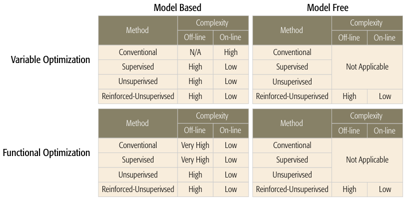
The on-line and off-line computational complexity of the DNN-based frameworks and the conventional optimization methods (e.g., convex optimization, SDR, and FEM) are summarized in Fig. 4.

References

- [1] F. Liang, C. Shen, W. Yu, and F. Wu, “Power control for interference management via ensembling deep neural networks,” in Proc. IEEE/CIC ICCC, 2019.
- [2] J. Gregory, Constrained optimization in the calculus of variations and optimal control theory. Chapman and Hall/CRC, 2018.
- [3] C. She, C. Yang, and T. Q. Quek, “Cross-layer optimization for ultra-reliable and low-latency radio access networks,” IEEE Trans. Wireless Commun., vol. 17, no. 1, pp. 127–141, Jan. 2017.
- [4] S. Boyd and L. Vandenberghe, Convex optimization. Cambridge Univ. Press, 2004.
- [5] O. C. Zienkiewicz, R. L. Taylor, P. Nithiarasu, and J. Zhu, The finite element method. McGraw-hill London, 1977, vol. 3.
- [6] C. Sun and C. Yang, “Unsupervised deep learning for ultra-reliable and low-latency communications,” in Proc. IEEE GLOBECOM, 2019.
- [7] H. Sun, X. Chen, Q. Shi, M. Hong, X. Fu, and N. D. Sidiropoulos, “Learning to optimize: Training deep neural networks for interference management,” IEEE Trans. Signal Process., vol. 66, no. 20, pp. 5438–5453, Oct. 2018.
- [8] M. Eisen, C. Zhang, L. F. Chamon, D. D. Lee, and A. Ribeiro, “Learning optimal resource allocations in wireless systems,” IEEE Trans. Signal Process., vol. 67, no. 10, pp. 2775–2790, May 2019.
- [9] L. Hoon, L. S. Hyun, and Q. Tony, “Constrained deep learning for wireless resource management,” in Proc. IEEE ICC, 2019.
- [10] F. D. Calabrese, L. Wang, E. Ghadimi, G. Peters, L. Hanzo, and P. Soldati, “Learning radio resource management in RANs: Framework, opportunities, and challenges,” IEEE Commun. Mag., vol. 56, no. 9, pp. 138–145, Sept. 2018.
- [11] R. S. Sutton and A. G. Barto, Reinforcement learning: An introduction. MIT Press Cambridge, 1998.
- [12] J. Garcıa and F. Fernández, “A comprehensive survey on safe reinforcement learning,” Journal of Machine Learning Research (JMLR), vol. 16, no. 1, pp. 1437–1480, 2015.
- [13] C. Sun and C. Yang, “Learning to optimize with unsupervised learning: Training deep neural networks for URLLC,” in Proc. IEEE PIMRC, 2019.
- [14] C. Sun, D. Liu, and C. Yang, “Model-free unsupervised learning for optimization problems with constraints,” in Proc. IEEE APCC, 2019.
- [15] T. P. Lillicrap, J. J. Hunt, A. Pritzel, N. Heess, T. Erez, Y. Tassa, D. Silver, and D. Wierstra, “Continuous control with deep reinforcement learning,” in Proc. ICLR, 2016.