Physically Plausible Spectral Reconstruction from RGB Images
Abstract
Recently Convolutional Neural Networks (CNN) have been used to reconstruct hyperspectral information from RGB images. Moreover, this spectral reconstruction problem (SR) can often be solved with good (low) error. However, these methods are not physically plausible: that is when the recovered spectra are reintegrated with the underlying camera sensitivities, the resulting predicted RGB is not the same as the actual RGB, and sometimes this discrepancy can be large. The problem is further compounded by exposure change. Indeed, most learning-based SR models train for a fixed exposure setting and we show that this can result in poor performance when exposure varies.
In this paper we show how CNN learning can be extended so that physical plausibility is enforced and the problem resulting from changing exposures is mitigated. Our SR solution improves the state-of-the-art spectral recovery performance under varying exposure conditions while simultaneously ensuring physical plausibility (i.e. the recovered spectra reintegrate to the input RGBs exactly).
I Introduction
Hyperspectral imaging devices are developed to capture high resolution radiance spectra at every pixel in an image, namely the hyperspectral images. These images often record additional scene information that are ‘invisible’ to human eyes and consumer RGB cameras (where the spectral information is recorded with only 3 intensity values per pixel), which has been found useful in numerous computer vision applications including remote sensing [40, 11, 19, 38, 10], anomaly detection [23] and medical imaging [44, 45], as well as computer graphics applications such as scene relighting [25] and digital art archiving [43].
Recent development in hyperspectral technology seeks faster image captures comparing to the conventional scanning-based techniques [18, 20]. Several attempts have been made for real-time multi-channel capturing [8, 42, 31, 37]. However, these devices are complicated and/or bulky that limits their usefulness. Other designs deploy novel optical components with specialized post-processing algorithms [12, 17, 6, 16, 27, 33, 47]. But, these devices trade off spatial resolution and/or light sensitivity for faster capturing speed.

Spectral reconstruction (SR) is an alternative approach to recording hyperspectral information, where hyperspectral images are recovered from RGB images [30, 3, 26, 24, 36, 15, 7, 26, 22, 4, 1, 15, 35, 5]. The idea is not as naïve as it might first appear. Indeed, we are expecting an RGB, which has just 3 numbers, to recover much more than 3 degrees of freedom in spectra. Fortunately, in natural scenes significant portion of the spectral variation is covered by its color appearance (i.e. the RGBs) [9], which makes it possible for learning approaches to give rather accurate spectral approximations. Recent approaches, leading by Convolutional Neural Networks (CNN), incorporate the images’ spatial context to further enhance the accuracy of spectral recovery.
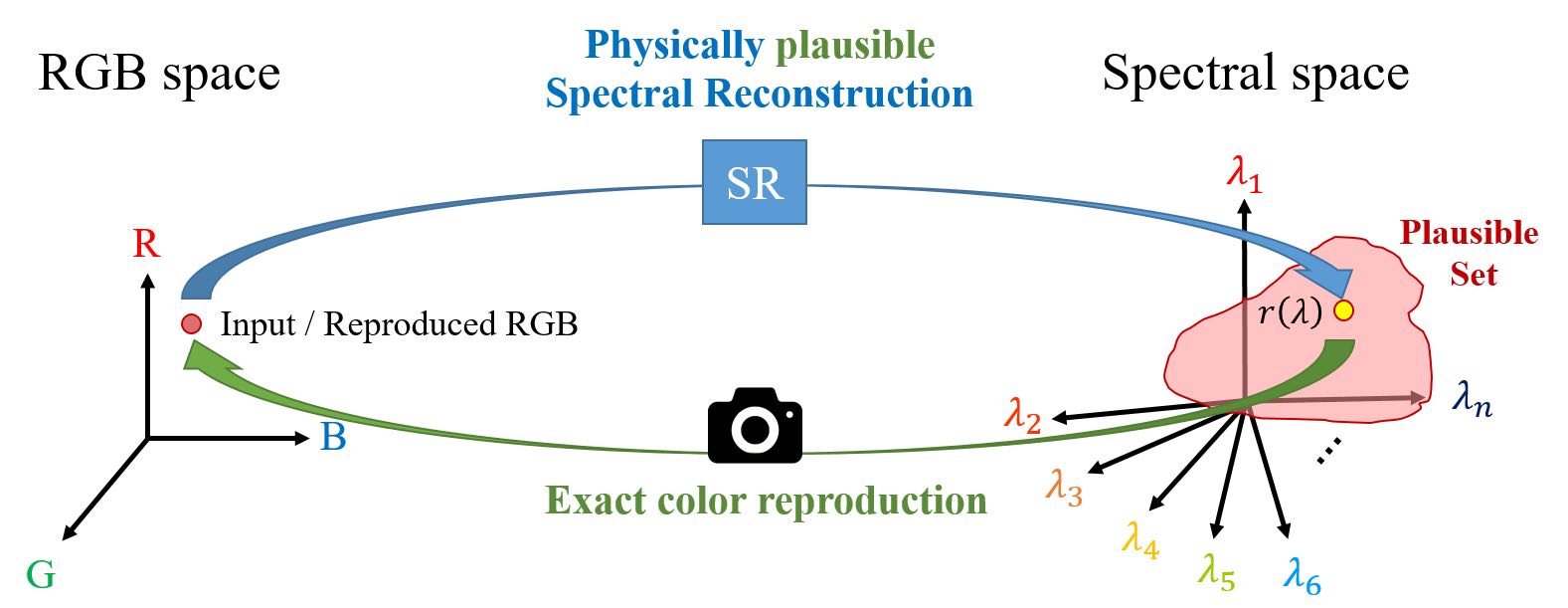
A key concern of this paper is the physical plausibility of the spectral reconstruction algorithms. If we physically measure the radiance spectra by an accurate hyperspectral camera, given the 3 spectral sensitivity functions of an RGB camera, we are guaranteed to produce the RGBs which the RGB camera will actually give. Unfortunately most - and all deep neural network based - spectral reconstruction algorithms do not ensure this property. Indeed, as we shall show in this paper, the predicted RGB can be quite far from the actual one. This is not just ‘unfortunate’ but completely missing out one of the key reasons we would like to use the spectral measurements: to predict what we see, for example to better predict our own color sensation when the viewing conditions change (i.e. the color correction problem).
In Figure 1 we illustrate the idea of ‘physical plausibility’. The physically plausible spectral reconstruction is illustrated in the top diagram. Here a radiance spectra (i.e. a spectral power distribution , see the right side of the image) is recovered from an RGB (the red point on the left in RGB space). Now we reintegrate the spectra with the camera’s spectral sensitivities - simulate taking a picture of this spectrum - which gives a predicted RGB. In this case the input RGB and the predicted counterpart are the same.
The diagram in the bottom half of Figure 1 shows a spectral recovery which produces incorrect color when reintegrated with the camera sensitivities. This ‘physically non-plausible spectral reconstruction’ is the norm (and is a feature exhibited by all deep network based algorithms we are aware of). Put bluntly, these algorithms provide the estimations of spectra which - because they do not reintegrate to the input RGB - must be the wrong answers.
In Figure 2 we show a pictorial example. In the bottom-middle panel we show two reconstructed spectra - red and purple dotted curves - having similar spectral difference from the ground-truth (blue solid curve). By integrating the sRGB display color matching functions given in the middle-top panel, the purple curve reproduces the background color exactly as the original painting on the left. In contrary, the red curve reproduces the image on the right, which shows significant background color shift.

The examples illustrated in Figures 1 and 2 show the advantage of incorporating the physics of image formation into learning-based methods for spectral reconstruction. Another related issue we also consider in this paper is exposure invariance. Clearly, if the light intensity in the scene changes, the ground-truth radiance spectra will be linearly scaled, and for linear RGB images (i.e. the camera raw data), the RGBs will also be scaled in the same way. However, as we later show in this paper this second physical reality is also not preserved in the state-of-the-art CNN models: these networks were trained for a single exposure condition and they perform poorly when a different exposure setting is tested.
This paper makes three main contributions:
- •
- •
We propose a novel framework which ensures exact color reproduction in CNN-based spectral reconstruction.
- •
We design a data augmentation process that maintains model stability over different exposure settings.
The rest of the paper is organized as follows. In section 2 we review the related field. In section 3 we show how we can solve the spectral reconstruction problem while ensuring physical plausibility. Implementation details are given in section 4. Experimental results are presented in section 5. The paper concludes in section 6.
II Related Work
Hyperspectral imaging. There exist technologies where hyperspectral images can be directly captured, and these include using a prism-mask system [8], multiple cameras [41, 31] and faced reflectors [37]. However, the practical applciation of these devices is limited by their complex configurations and/or their physical bulkiness. Alternately, in compressive imaging, a scene’s spectral information is encoded in alternative forms on the sensed 2-D images. But, there is the overhead of decompressing the signal. Examples include multi-spectral color filter array [12], coded aperture [6, 16, 17], diffractive gratings [27], digital micro-mirror device [33] and most recently random printed mask [47]. Other problems inherent in compressive sensing are the need for specialized optics and the inherent trade-off between the number of sensors and/or light sensitivity and the spatial resolution.
Spectral reconstruction (SR). Rather than building new hardware for capturing hyperspectral images, spectral reconstruction attempts to map RGB images to their spectral counterparts. Shallow-learned methods - of which sparse coding is the best example [4, 1] - have the advantage of model simplicity and quick training. However, these models is effectively implementing a ‘one-to-one’ lookup table, which contradicts the fact that many (in fact infinite) spectra can reproduce the same RGB.
In the CNN approach the implementation complexity is much higher as so the hardware requirements but the reconstruction is richer. The promise of these methods is that, in an intermediate representation, they might identify scene contents which are associated with the target spectra and then effectively use these information in the recovery process. Indeed, it is well known that faces, chlorophyl (in foliage) and daylights have very characteristic shapes (amongst other scene features). Of the current developments, deep neural networks [3, 24, 36, 15, 35] provide the leading performance in spectral reconstruction.
Physical plausibility. In this paper we address the importance that, as an alternative way of getting hyperspectral information, a spectral reconstruction algorithm should always produce physically plausible radiance predictions which can be reintegrated to the same RGB values as they are recovered from.
Interestingly, some of the early models can already provide accurate color reproduction (but much poorer spectral recovery comparing to the recent CNN methods). For example, using weighted-PCA based on color differences [2] and colorimetrically correcting the linear regression spectral recovery (i.e. pseudo-inverse) [46]. Furthermore, sparse coding methods [4, 1] can also provide rather accurate color reproduction by virtue of their fundamental ‘neighbor embedding’ assumption [39]. Finally, the complex and computationally laborious Bayesian inference method [29] was also introduced where physical plausibility is ensured.
However, in the recent NTIRE 2018 Challenge on Spectral Reconstruction from RGB Images (hereinafter abbreviated as NTIRE2018) [5], all 12 leading entries out of 73 attendants (on the ‘Clean Track’) involve the implementation of deep neural networks. None of these methods explicitly ensure the spectra can reintegrate to the input RGBs.
Exposure invariance. In many learning-based computer vision tasks, the model stability over intensity change are considered; that is, the model are ensured to work well even as the scene exposure changes. However, Lin and Finlayson [28] demonstrated that leading spectral reconstruction models in NTIRE2018 perform poorly in different exposure settings, and this has raised a concern that many modern developments of spectral reconstruction may not work in the wild where exposure can vary.
III Physically Plausible Spectral Reconstruction
At each pixel of a hyperspectral image, a high-resolution radiance spectrum is recorded. The corresponding RGB image is simulated by calculating the inner products between the measured radiance spectra and the spectral sensitivity functions of the RGB camera:
| (1a) | |||
| where refer to the red, green and blue channels of the RGB image, , and are respectively the -th camera response, the -th camera sensitivity function and the radiance function, denotes the wavelength dimension, and is the visible spectrum. Of course for this inner-product model (as oppose to an integral) of image formation to work, we must sample the spectra at a sufficient resolution across the visible spectrum. In all simulations we report later in this paper, we assume the visible spectrum runs from 400 through 700 nanometers, and the spectra are sampled every 10 nanometers (this is the common assumption made in most studies, including the NTIRE2018 [5]). | |||
Let us vectorize the above equation:
| (1b) |
where is the -dimensional RGB vector, is the -dimensional radiance spectra with to be the number of spectral bands, and is an matrix with its columns to be the three distinct camera sensitivity functions.
In the ordinary spectral reconstruction framework, the radiance spectrum is recovered from the RGB camera response : the spectral reconstruction algorithm searches for the best solution to within the entire spectral space (i.e. ) that statistically minimizes the distance error between the recovered and ground-truth radiance spectra. However, this framework does not ensure that the reconstructed must reproduce - the algorithm may find a solution which is spectrally close to the ground-truth but reproduces distant color (as per the example we showed in Figure 2).
Let us now develop a method to constrain the algorithm only to search for the estimated radiance within the set of spectra that integrates to the correct RGB. For this purpose, we propose a plausible set concept, which is defined as the set of all spectra that integrate to a target RGB.
The derivation of our plausible set is analogous to, but simpler than, the metamer set in [14, 29], while their focus was on the reflectance set instead of our case on the radiance set.
III-A The Plausible Set
Given known camera sensitivity functions , the plausible set is defined as:
| (2) |
Geometrically, the outcome of an inner product is only affected by the parts of the two vectors that are ‘parallel’ to each other, whereas the ‘perpendicular’ part do not contribute to the product.
Given this view, the constraint in effect separates into two parts: the part that is spanned by the column vectors of which contributes to , and the part lies in the null-space of which yields zero projection. That is,
| (3) |
subject to
| (4a) | ||||
| (4b) | ||||
| and | ||||
| (4c) | ||||
The component can be derived directly by the subspace projection. The projection matrix with respect to is written as:
| (5) |
such that
| (6) |
Next, we enforce our desired constraint on , which gives
| (7) |
It is important to see that the derived is fixed given and , which implies that all shares the same and only the component determines the difference between the radiance in set .
On the other hand, can be any vector in the null space of , which is spanned by linearly independent bases that are orthogonal to all column vectors of . This set of bases can be obtained by finding the non-trivial solutions of in Equation (4b), or by calculating the basis vectors that span ( is the identity matrix), which is the projection matrix with respect to all other dimensions in that are orthogonal to the column space of . In either way, we get a set of null-space bases, and every can be uniquely derived by a linear combination of them:
| (8) |
where is an matrix with its columns to be the null-space basis vectors. We call the null-space coefficients. Finally, we reach the following definition of :
| (9) |
where all , and are known factors, leaving to be the only variation within the plausible set .
In the next part of this section, we are going to introduce our physically plausible spectral reconstruction via the null-space coefficients reconstruction.
III-B Reconstructing the Null-space Coefficients
Recall Equation (1a) and (1b), given a ground-truth radiance , the corresponding RGB is calculated by . This indicates that is a member of , in which it corresponds to one unique , denoted as . Based on which, we further translate our goal of making the spectral reconstruction algorithm search for the reconstruction in , into seeking the null-space coefficients in which best approximates . Training the spectral reconstruction algorithm such that
| (10) |
the reconstructed spectrum is then derived by
| (11) |
So far, the idea behind our physically plausible framework for spectral reconstruction has been established. Still, for CNN models the ground-truth labels are necessary, which means we are yet to calculate from the in the hyperspectral images.
In Equation (5) we calculated the projection matrix which projects onto the column space of that derives . Likewise, to derive we seek the projection of onto the column space of the . The null-space projection matrix can be written as:
| (12) |
(which is equivalent to ), such that
| (13) |
Together with Equation (8), we get
| (14) |
Finally, since the columns of (i.e. the null-space basis vectors) are linearly-independent, we derive
| (15) |
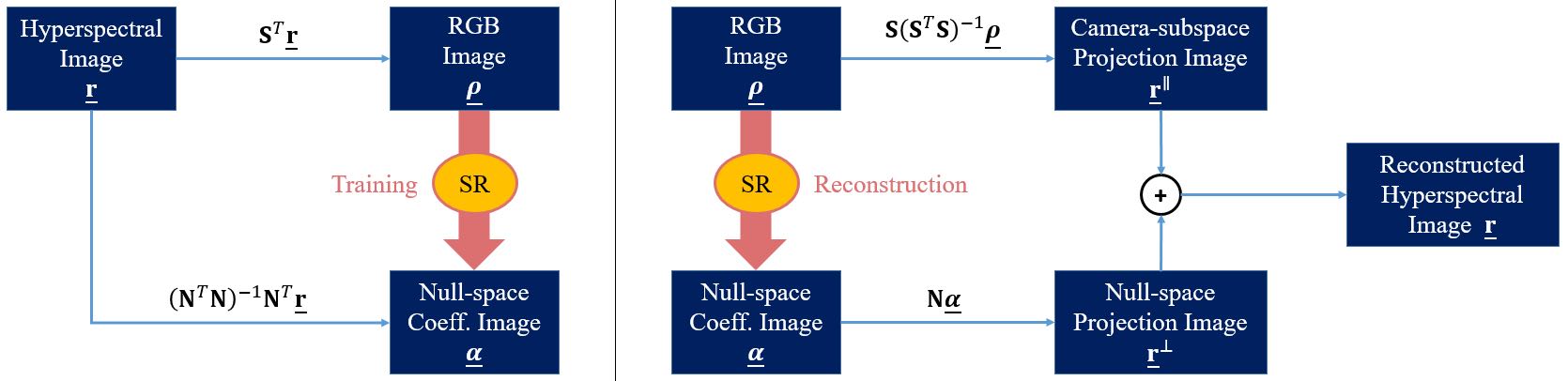
Figure 3 summarizes the framework of our physically plausible spectral reconstruction. In the reconstruction stage, the camera-subspace projection is calculated directly from the RGB input and the spectral reconstruction algorithm only concerns the recovery of the null-space projection . As the color reproduction of the reconstructed hyperspectral image only depends on (Equation (4a) and (4b)), the reconstructed hyperspectral image is ensured to reproduce exactly the input RGB image. In the next section we are going to integrate this framework with the state-of-the-art spectral reconstruction model based on CNN.
IV Implementation

We build our models based on the HSCNN-R architecture, which is the 2nd place entry of the NTIRE2018 [5, 35] (whose performance is similar to the 1st place HSCNN-D model; we use the 2nd place architecture simply because it was simpler in our development environment). As illustrated in Figure 4, the HSCNN-R model adopts a deep residual learning framework [21]. Each of the residual blocks is constructed with two convolutional layers and one ReLU layer. The model also adopts a global residual learning structure. All convolutional kernels are set to .
On training and reconstruction, the network maps RGB image patches to the corresponding -channel hyperspectral patches (the spectral dimension runs from 400 to 700 with 10 sampling intervals). The final image is decided by the reconstruction outcome of 3 HSCNN-R networks with different filter numbers in each layer (64, 256 and 256) and depths (34, 20, and 30).
In this paper, we aim for two improvements on HSCNN-R: (1) perfect color reproduction and (2) robustness against exposure change. For the former, we integrate our physically plausible framework to HSCNN-R, and for the latter, we propose a new data augmentation process. To study the effects of both improvements, 3 new models listed in Table I are trained.
| Model | Physically | Data |
|---|---|---|
| Plausible | Augmentation | |
| V | ||
| V | ||
| V | V |
IV-A Physically Plausible HSCNN-R
In the original HSCNN-R model, the output layer corresponds to a hyperspectral image patch with spectral dimensions. To accommodate our physically plausible framework in HSCNN-Rp and HSCNN-Rpd, we reduce the spectral dimension from to in the output layer for recovering the image of null-space coefficients ( is -dimensional with ).
Unlike the original hyperspectral data which only contains positive values, the null-space coefficients allow negative entries, and this is not permitted for the ReLU output layer in the HSCNN-R architecture. As a result, it is necessary to re-center the ground-truth such that the negative values are prevented.
In our implementation, we found that empirically the entries of the ground-truth range between and . Hence, in the training stage of HSCNN-Rp we adopt a re-centering:
| (16) |
The reverse function is used in the reconstruction stage to center the targeted back from . As we will mention later the HSCNN-Rpd model requires a different re-centering function due to the implementation of our data augmentation process.
The rest of the hyperparameters of HSCNN-Rp are kept the same as the original HSCNN-R model [35]. Our HSCNN-Rp is expected to provide absolute color reproduction. However, as shown in [28], the original HSCNN-R is not robust against intensity change, and this implies that HSCNN-Rp also may not perform well in spectral recovery when the testing exposure condition varies.
IV-B Intensity-scaling Data Augmentation
We create the augmented data by simulating ‘brighter’ and ‘dimmer’ RGB images from the ground-truth hyperspectral images. Instead of generating all the new data before training the model, we draw different scaling constants in real time during training: all input image patches (and the same patch in different training epochs) are scaled differently, which allows the network to see more intensity variation in the data.
Furthermore, since a spectral reconstruction algorithm can be potentially implemented on an RGB camera, we want to especially ensure that, when adjusting the standard exposure settings in the RGB cameras (i.e. the aperture size and shutter speed) the trained model performs equally well. We remind that these settings by convention follow geometric progressions; more precisely, the available aperture sizes normally follows a sequential scaling change by , and the shutter speed is adjusted by a factor of 2 between adjacent modes. Based on this fact, we propose to draw the scaling constants from a uniform distribution on a log scale:
| (17) |
In our implementation, we set such that the scaling factor is bounded by .
For comparison, we train another intermediate model, HSCNN-Rd, which only adopts the intensity-scaling data augmentation. This model is refined from the pre-trained HSCNN-R provided in [35], and all hyperparameters are kept the same.
Model Original exposure () Half exposure () Double exposure () MRAE () MRAE () MRAE () Mean WC Mean WC Mean WC Mean WC Mean WC Mean WC HSCNN-D 0.51 10.18 1.19 14.09 1.75 11.08 14.87 48.24 0.51 9.17 5.79 23.36 HSCNN-R 0.49 13.10 1.35 23.84 1.98 13.81 17.41 71.94 0.67 9.45 5.86 24.95 HSCNN-R 0.00 0.00 1.73 19.31 0.00 0.00 14.23 37.94 0.00 0.00 6.43 24.84 HSCNN-R 0.26 8.98 2.77 19.78 0.25 8.92 2.78 19.83 0.26 9.07 2.77 19.73 HSCNN-Rpd 0.00 0.00 2.80 23.93 0.00 0.00 2.91 23.89 0.00 0.00 2.78 24.09
On the other hand, to apply this new data augmentation framework on the physically plausible model, we need to adjust the re-centering function to accommodate the change in range of the entries of . In our case, as :
| (18) |
Additionally, to make the model converge efficiently, we set the adaptive learning rate to follow a polynomial decay with the power of (instead of the original ). This final model is referred to as HSCNN-Rpd.
V Experiment
V-A Experimental Setup
We trained our new models (as listed in Table I) based on the ICVL database [4] (201 hyperspectral images), where we randomly split the database into 100 images for training, 50 for validation and 50 for evaluation. The CIE 1964 color matching functions [13] were selected as the camera sensitivity functions, by which the ground-truth RGBs (i.e. the CIEXYZ color coordinates) were simulated. We also tested the original HSCNN-D and HSCNN-R models (the pre-trained networks in [35] were directly used) to compare with our new models.
Our experiment concerns the performances of the models in terms of (1) color reproduction, (2) spectral recovery and (3) both performances under different exposure settings. We select the following error metrics:
- •
Color difference: CIE 1976 color difference
(19)
- •
Spectral difference: Mean Relative Absolute Error
(20)
Equation (19) shows the definition of the CIE 1976 color difference formula [32], where and are the CIELAB color coordinates of the ground-truth and reconstructed RGB colors, respectively. The transformation between CIEXYZ and CIELAB requires the normalization by the ‘white point’ coordinates (i.e. the illumination color), for which we hand-craft the white points of each images by selecting the RGB of the brightest achromatic pixel.
In Equation (20), respectively and refers to the ground-truth and reconstructed radiance spectra, and is the number of spectral bands. The division is component-wise and the norm is calculated.
Note that both of the above metrics are pixel-wisely defined, which means the performance of each pixel in an image is considered independently. In addition, since both metrics involve normalization of the reference intensity: for the illumination white-point coordinates are divided, and for MRAE the spectral difference is divided by the ground-truth spectrum. This ensures that our performance measurements are independent to the overall intensity of the compared targets.
We test all models under 3 exposure settings: the original, half and double exposure. For each testing exposure, we uniformly scale-up all the evaluation images with the same scaling constant (respectively = 1, 0.5 and 2), and the reconstructed hyperspectral images are compared with the ground-truth hyperspectral images scaled by the same constant.
V-B Result and Discussion
The performance statistics are shown in Table II. We show the mean and the worst-case (WC) performance of the models. The ‘worst case’ is defined per image as the averaged error of ‘the worst 1000 pixels’ (the image dimension is around ), and the worst-case performance given in Table II refers to the mean worst-case error over all evaluation set.
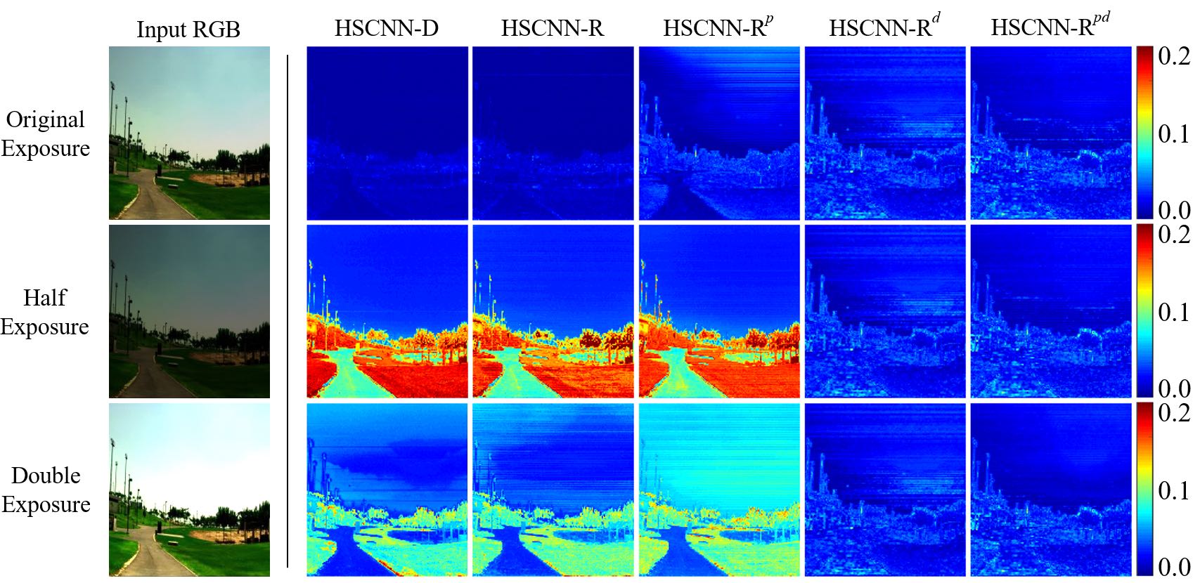
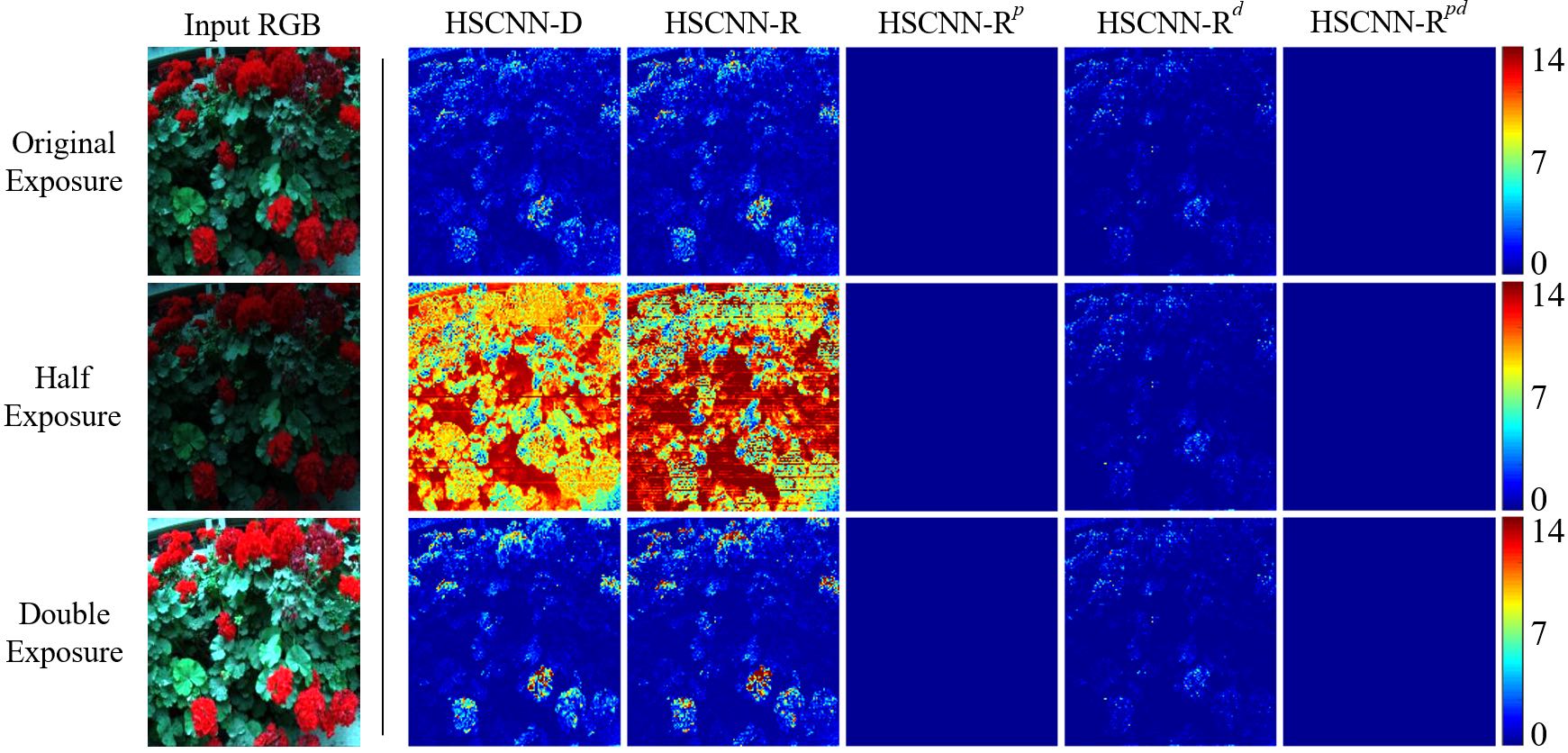
First, we see that the state-of-the-art HSCNN-D and HSCNN-R are not physically plausible. Indeed, the worst-case of these models are significant (referring to [34] human observers can sense noticeable difference above ). Our physically plausible HSCNN-Rp not only provides zero error in color reproduction, but also significantly improves the worst-case performance in terms of spectral recovery over the original HSCNN-R. However, as shown in Figure 6, HSCNN-Rp and the original models provide poor spectral recovery performance when half and double exposure settings are applied.
Next, we can see very clearly in Figure 6 and 7 that standalone HSCNN-Rd (without the physically plausible training) shows great advantage over original HSCNN-D and HSCNN-R in both the spectral recovery and color reproduction performance when exposure condition changes. However, the worst-case color reproduction performance of HSCNN-Rd is still sub-optimal.
Lastly, we want to ‘jointly’ consider the performance in spectral recovery and color reproduction. Frankly speaking, it is not possible to strictly say which performance is more important than the other. We also remark that depending on different applications, this relative importance can vary drastically. Despite of this, we can combine the two metrics with an adjustable relative weight, to see the model performance in all different cases of relative importance. Define a joint metric :
| (21) |
the joint metric in effect describes the ‘competition’ in importance between the two concerned metrics. We show two comparisons. First we show the mean MRAE against the mean in the top panel of Figure 5, and the worst-case MRAE competed with the worst-case in the bottom panel. Note that for each model we average the performances under the 3 testing exposure conditions, and we normalize all performances by the average performance across models (this is for making MRAE and in the same order of magnitude). We show that in both cases, either mean or worst-case performances, our proposed HSCNN-Rpd performs the best overall.


VI Conclusion
Spectral reconstruction (SR) studies the mapping from RGB to hyperspectral images, which is regarded as a promising solution to low-cost, snapshot and high resolution hyperspectral camera. In the recent development of spectral reconstruction, leading models are based on Convolutional Neural Networks (CNN), providing remarkable spectral recovery performance. However, these models only aim to minimize the spectral recovery errors without ensuring the physical plausibility of the output spectra. Physical plausibility is defined as ensuring the recovered spectrum integrates (using the underlying camera sensors) to the same RGB as it is recovered from. Existing method, which do not have this property, estimate RGBs which are significantly different from those found in the original image.
In this paper we developed a physically plausible Spectral reconstruction framework. Our insight is that all plausible spectra can be represented by a fixed camera-subspace projection spectrum defined by a linear combination of camera spectral sensitivities, and a null-space spectrum which do not contribute to the color formation. Relative to this insight, the spectral recovery problem sets out to reconstruct the null-space spectra from the RGB (instead of the original RGB to radiance mapping), such that the physical plausibility of the predicted radiance is guaranteed. Finally, we also addressed the issue of exposure invariance in spectral reconstruction [28], by proposing a new data augmentation framework to ensure the model robustness against intensity variations. As the exposure changes, our models provide leading performance considering both spectral recovery and color reproduction.
References
- [1] Jonas Aeschbacher, Jiqing Wu, and Radu Timofte. In defense of shallow learned spectral reconstruction from rgb images. In Proceedings of the IEEE International Conference on Computer Vision, pages 471–479, 2017.
- [2] Farnaz Agahian, Seyed Ali Amirshahi, and Seyed Hossein Amirshahi. Reconstruction of reflectance spectra using weighted principal component analysis. Color Research & Application, 33(5):360–371, 2008.
- [3] Aitor Alvarez-Gila, Joost Van De Weijer, and Estibaliz Garrote. Adversarial networks for spatial context-aware spectral image reconstruction from rgb. In Proceedings of the IEEE International Conference on Computer Vision, pages 480–490, 2017.
- [4] Boaz Arad and Ohad Ben-Shahar. Sparse recovery of hyperspectral signal from natural rgb images. In European Conference on Computer Vision, pages 19–34. Springer, 2016.
- [5] Boaz Arad, Ohad Ben-Shahar, and Radu Timofte. Ntire 2018 challenge on spectral reconstruction from rgb images. In Proceedings of the IEEE Conference on Computer Vision and Pattern Recognition Workshops, pages 929–938, 2018.
- [6] Henry Arguello and Gonzalo R Arce. Colored coded aperture design by concentration of measure in compressive spectral imaging. IEEE Transactions on Image Processing, 23(4):1896–1908, 2014.
- [7] Bin Cao, Ningfang Liao, and Haobo Cheng. Spectral reflectance reconstruction from rgb images based on weighting smaller color difference group. Color Research & Application, 42(3):327–332, 2017.
- [8] Xun Cao, Hao Du, Xin Tong, Qionghai Dai, and Stephen Lin. A prism-mask system for multispectral video acquisition. IEEE transactions on pattern analysis and machine intelligence, 33(12):2423–2435, 2011.
- [9] Ayan Chakrabarti and Todd Zickler. Statistics of real-world hyperspectral images. In CVPR 2011, pages 193–200. IEEE, 2011.
- [10] Chen Chen, Wei Li, Hongjun Su, and Kui Liu. Spectral-spatial classification of hyperspectral image based on kernel extreme learning machine. Remote Sensing, 6(6):5795–5814, 2014.
- [11] Yushi Chen, Xing Zhao, and Xiuping Jia. Spectral–spatial classification of hyperspectral data based on deep belief network. IEEE Journal of Selected Topics in Applied Earth Observations and Remote Sensing, 8(6):2381–2392, 2015.
- [12] Claudia V Correa, Henry Arguello, and Gonzalo R Arce. Snapshot colored compressive spectral imager. JOSA A, 32(10):1754–1763, 2015.
- [13] Commission Internationale de l’Eclairage. Cie proceedings (1964) vienna session, committee report e-1.4. 1. 1964.
- [14] Graham D Finlayson and Peter Morovic. Metamer sets. JOSA A, 22(5):810–819, 2005.
- [15] Ying Fu, Tao Zhang, Yinqiang Zheng, Debing Zhang, and Hua Huang. Joint camera spectral sensitivity selection and hyperspectral image recovery. In Proceedings of the European Conference on Computer Vision (ECCV), pages 788–804, 2018.
- [16] Laura Galvis, Daniel Lau, Xu Ma, Henry Arguello, and Gonzalo R Arce. Coded aperture design in compressive spectral imaging based on side information. Applied optics, 56(22):6332–6340, 2017.
- [17] Hans Garcia, Claudia V Correa, and Henry Arguello. Multi-resolution compressive spectral imaging reconstruction from single pixel measurements. IEEE Transactions on Image Processing, 27(12):6174–6184, 2018.
- [18] Nahum Gat. Imaging spectroscopy using tunable filters: a review. In Wavelet Applications VII, volume 4056, pages 50–64. International Society for Optics and Photonics, 2000.
- [19] Pedram Ghamisi, Mauro Dalla Mura, and Jon Atli Benediktsson. A survey on spectral–spatial classification techniques based on attribute profiles. IEEE Transactions on Geoscience and Remote Sensing, 53(5):2335–2353, 2014.
- [20] Robert O Green, Michael L Eastwood, Charles M Sarture, Thomas G Chrien, Mikael Aronsson, Bruce J Chippendale, Jessica A Faust, Betina E Pavri, Christopher J Chovit, Manuel Solis, et al. Imaging spectroscopy and the airborne visible/infrared imaging spectrometer (aviris). Remote sensing of environment, 65(3):227–248, 1998.
- [21] Kaiming He, Xiangyu Zhang, Shaoqing Ren, and Jian Sun. Deep residual learning for image recognition. In Proceedings of the IEEE conference on computer vision and pattern recognition, pages 770–778, 2016.
- [22] Ville Heikkinen, Reiner Lenz, Tuija Jetsu, Jussi Parkkinen, Markku Hauta-Kasari, and Timo Jääskeläinen. Evaluation and unification of some methods for estimating reflectance spectra from rgb images. JOSA A, 25(10):2444–2458, 2008.
- [23] James A Jablonski, Trevor J Bihl, and Kenneth W Bauer. Principal component reconstruction error for hyperspectral anomaly detection. IEEE Geoscience and Remote Sensing Letters, 12(8):1725–1729, 2015.
- [24] Sriharsha Koundinya, Himanshu Sharma, Manoj Sharma, Avinash Upadhyay, Raunak Manekar, Rudrabha Mukhopadhyay, Abhijit Karmakar, and Santanu Chaudhury. 2d-3d cnn based architectures for spectral reconstruction from rgb images. In Proceedings of the IEEE Conference on Computer Vision and Pattern Recognition Workshops, pages 844–851, 2018.
- [25] Antony Lam and Imari Sato. Spectral modeling and relighting of reflective-fluorescent scenes. In Proceedings of the IEEE Conference on Computer Vision and Pattern Recognition, pages 1452–1459, 2013.
- [26] Jinxing Liang and Xiaoxia Wan. Optimized method for spectral reflectance reconstruction from camera responses. Optics Express, 25(23):28273–28287, 2017.
- [27] Xing Lin, Yebin Liu, Jiamin Wu, and Qionghai Dai. Spatial-spectral encoded compressive hyperspectral imaging. ACM Transactions on Graphics (TOG), 33(6):233, 2014.
- [28] Yi-Tun Lin and Graham D Finlayson. Exposure invariance in spectral reconstruction from rgb images. In Color and Imaging Conference, volume 2019, pages 284–289. Society for Imaging Science and Technology, 2019.
- [29] Peter Morovic and Graham D Finlayson. Metamer-set-based approach to estimating surface reflectance from camera rgb. JOSA A, 23(8):1814–1822, 2006.
- [30] Rang MH Nguyen, Dilip K Prasad, and Michael S Brown. Training-based spectral reconstruction from a single rgb image. In European Conference on Computer Vision, pages 186–201. Springer, 2014.
- [31] Wug Seoung Oh, Michael S Brown, Marc Pollefeys, and Seon Joo Kim. Do it yourself hyperspectral imaging with everyday digital cameras. In Proceedings of the IEEE Conference on Computer Vision and Pattern Recognition, pages 2461–2469, 2016.
- [32] Alan R Robertson. The cie 1976 color-difference formulae. Color Research & Application, 2(1):7–11, 1977.
- [33] Hoover Rueda, Henry Arguello, and Gonzalo R Arce. Dmd-based implementation of patterned optical filter arrays for compressive spectral imaging. JOSA A, 32(1):80–89, 2015.
- [34] Gaurav Sharma and Raja Bala. Digital color imaging handbook. CRC press, 2002.
- [35] Zhan Shi, Chang Chen, Zhiwei Xiong, Dong Liu, and Feng Wu. Hscnn+: Advanced cnn-based hyperspectral recovery from rgb images. In Proceedings of the IEEE Conference on Computer Vision and Pattern Recognition Workshops, pages 939–947, 2018.
- [36] Tarek Stiebel, Simon Koppers, Philipp Seltsam, and Dorit Merhof. Reconstructing spectral images from rgb-images using a convolutional neural network. In Proceedings of the IEEE Conference on Computer Vision and Pattern Recognition Workshops, pages 948–953, 2018.
- [37] Tsuyoshi Takatani, Takahito Aoto, and Yasuhiro Mukaigawa. One-shot hyperspectral imaging using faced reflectors. In Proceedings of the IEEE Conference on Computer Vision and Pattern Recognition, pages 4039–4047, 2017.
- [38] Chao Tao, Hongbo Pan, Yansheng Li, and Zhengrou Zou. Unsupervised spectral–spatial feature learning with stacked sparse autoencoder for hyperspectral imagery classification. IEEE Geoscience and remote sensing letters, 12(12):2438–2442, 2015.
- [39] Radu Timofte, Vincent De Smet, and Luc Van Gool. A+: Adjusted anchored neighborhood regression for fast super-resolution. In Asian conference on computer vision, pages 111–126. Springer, 2014.
- [40] Miguel A Veganzones, Guillaume Tochon, Mauro Dalla-Mura, Antonio J Plaza, and Jocelyn Chanussot. Hyperspectral image segmentation using a new spectral unmixing-based binary partition tree representation. IEEE Transactions on Image Processing, 23(8):3574–3589, 2014.
- [41] Lizhi Wang, Zhiwei Xiong, Dahua Gao, Guangming Shi, and Feng Wu. Dual-camera design for coded aperture snapshot spectral imaging. Applied optics, 54(4):848–858, 2015.
- [42] Lizhi Wang, Zhiwei Xiong, Dahua Gao, Guangming Shi, Wenjun Zeng, and Feng Wu. High-speed hyperspectral video acquisition with a dual-camera architecture. In Proceedings of the IEEE Conference on Computer Vision and Pattern Recognition, pages 4942–4950, 2015.
- [43] Peng Xu, Haisong Xu, Changyu Diao, and Zhengnan Ye. Self-training-based spectral image reconstruction for art paintings with multispectral imaging. Applied optics, 56(30):8461–8470, 2017.
- [44] Yanbo Zhang, Xuanqin Mou, Ge Wang, and Hengyong Yu. Tensor-based dictionary learning for spectral ct reconstruction. IEEE transactions on medical imaging, 36(1):142–154, 2016.
- [45] Yi Zhang, Yan Xi, Qingsong Yang, Wenxiang Cong, Jiliu Zhou, and Ge Wang. Spectral ct reconstruction with image sparsity and spectral mean. IEEE transactions on computational imaging, 2(4):510–523, 2016.
- [46] Yonghui Zhao and Roy S Berns. Image-based spectral reflectance reconstruction using the matrix r method. Color Research & Application, 32(5):343–351, 2007.
- [47] Yuanyuan Zhao, Hui Guo, Zhan Ma, Xun Cao, Tao Yue, and Xuemei Hu. Hyperspectral imaging with random printed mask. In Proceedings of the IEEE Conference on Computer Vision and Pattern Recognition, pages 10149–10157, 2019.