3D UAV Trajectory and Communication Design for Simultaneous Uplink and Downlink TransmissionThanks: This paper has been accepted by IEEE Transactions on Communications. Manuscript received January 02, 2020; revised April 27, and accepted June 12, 2020. This work was supported by the National Natural Science Foundation of China under Grants U1936201 and 61971128, Scientific Research Foundation of Graduate School of Southeast University under Grand YBPY1859, and the National Key Research and Development Program of China under Grant SQ2019YFB180141-01. The associate editor coordinating the review of this paper and approving it for publication was Mehdi Bennis. (Corresponding author: Luxi Yang.)Thanks: M. Hua, and L. Yang are with the School of Information Science and Engineering, Southeast University, Nanjing 210096, China (e-mail: {mhua, lxyang}@seu.edu.cn).Thanks: Q. Wu is with the State Key Laboratory of Internet of Things for Smart City and Department of Electrical and Computer Engineering, University of Macau, Macao, China (email: qingqingwu@um.edu.mo).Thanks: A. L. Swindlehurst is with the Center for Pervasive Communications and Computing, University of California at Irvine, Irvine, CA 92697 USA (e-mail: swindle@uci.edu).

With continuing communication device miniaturization and the increased endurance of unmanned aerial vehicles (UAVs), new civilian-use markets are emerging for UAVs beyond military applications, including examples such as emergency search, forest fire detection, cargo transport, etc. Particularly, UAVs are envisioned as a key component of future wireless network technologies that will expand network coverage and improve system throughput [1, 2, 3]. Compared with terrestrial base stations (BSs) whose the locations are pre-determined and fixed, UAVs can adaptively control its position to react as needed to requests for on-demand services [4, 5, 6, 7, 8, 9, 10].

There are two main paradigms for the integration of UAVs in the traditional networks, namely UAV-aided wireless networks and cellular-connected UAV networks [11, 12, 13, 14, 15, 16, 17, 18]. In the UAV-aided wireless communication scenario, the UAV generally acts as a mobile BS equipped with a communication transceiver to provide seamless wireless services or to collect the data from the ground nodes. UAVs are especially well suited for data collection in sensor networks where the nodes are widely dispersed over a large area [11, 12, 13, 14]. The sensor nodes (SNs) are typically battery operated, and cannot transmit continuously. Rather than installing dedicated infrastructure, in delay-tolerant applications it is more cost effective to deploy UAVs to visit the SNs and collect the data in a sense-and-carry fashion. In the cellular-connected UAV communication networks, UAVs are regarded as new aerial users that access the cellular network from the sky for communications [15, 16, 17, 18]. In [19], an in-depth analysis of integration of cellular-connected UAV into the existing wireless networks is provided from the perspectives of multiple metrics. Such UAVs can achieve high data rates with low latency due to the high probability of dominant line-of-sight (LoS) propagation paths with its communication targets.

Despite promising opportunities for UAVs like those mentioned above, some key challenges remain to be addressed in order to effectively use them to realize seamless connectivity and ultra reliable communication in the future. Recently, UAV deployment and trajectory designs for sensing and communications have received great attention [20, 21, 22, 23, 24, 25, 26, 27, 28, 29, 30]. The deployment of a single UAV was investigated in [20, 21, 22], especially [22] derived analytical expressions for the optimal UAV altitude that minimizes the system outage probability by using stochastic geometry theory. The deployment of multiple UAVs for either maximizing the coverage area or system throughput was investigated in [23] and [24], respectively. The initial 2D UAV trajectory optimization was studied in [26], where the authors divided the continuous trajectory into multiple discrete segments and solved the discrete problem by convex optimization techniques. Then, 3D trajectory design has been studied in [27] and [28]. The goal of [27] was to maximize the minimum average data collection rate from all SNs by optimizing the 3D UAV trajectory under the assumption of Rician fading channels, while the optimal 3D trajectory was obtained by applying monotonic optimization theory in [28]. The problem of multiple UAVs simultaneously serving multiple SNs was first studied in [29] and [30]. In [29], the UAV transmit power and trajectory were optimized to alleviate the interference received by the SNs and maximize the minimum achieved rate from all the SNs. In [30], the authors studied multiple-UAV cooperative secure transmission problem by jointly optimizing the UAV trajectory and transmit power.

While the above work has studied the typical UAV-aided wireless communication network either in the uplink transmission or downlink transmission, question of how to integrate the operation of simultaneous uplink and downlink transmission has not been addressed and remains an open problem. To fill this gap, we study a general heterogeneous network that consists of these two networks. For the downlink transmission network, UAV acts as a disseminator, referred to as UAV-AP, to disseminate data to the ground access point (AP) (Note that the AP is also a type of SNs, we name it as AP to distinguish uplink SNs). For the UAV-BS based network, the UAV acts as a mobile base station (BS), referred to as UAV-BS, to collect data from the uplink SNs. We aim to maximize the sum system throughput, including contributions from both UAV-BS and UAV-AP operations, by jointly optimizing the 3D UAV-BS/UAV-AP trajectory, communication scheduling, and UAV-AP/SN transmit power. We propose an efficient iterative algorithm to address the problem and obtain a locally optimal solution. In addition, for the special case where both UAVs’ trajectories are pre-determined, we obtain a globally optimal solution by applying monotonic optimization theory.

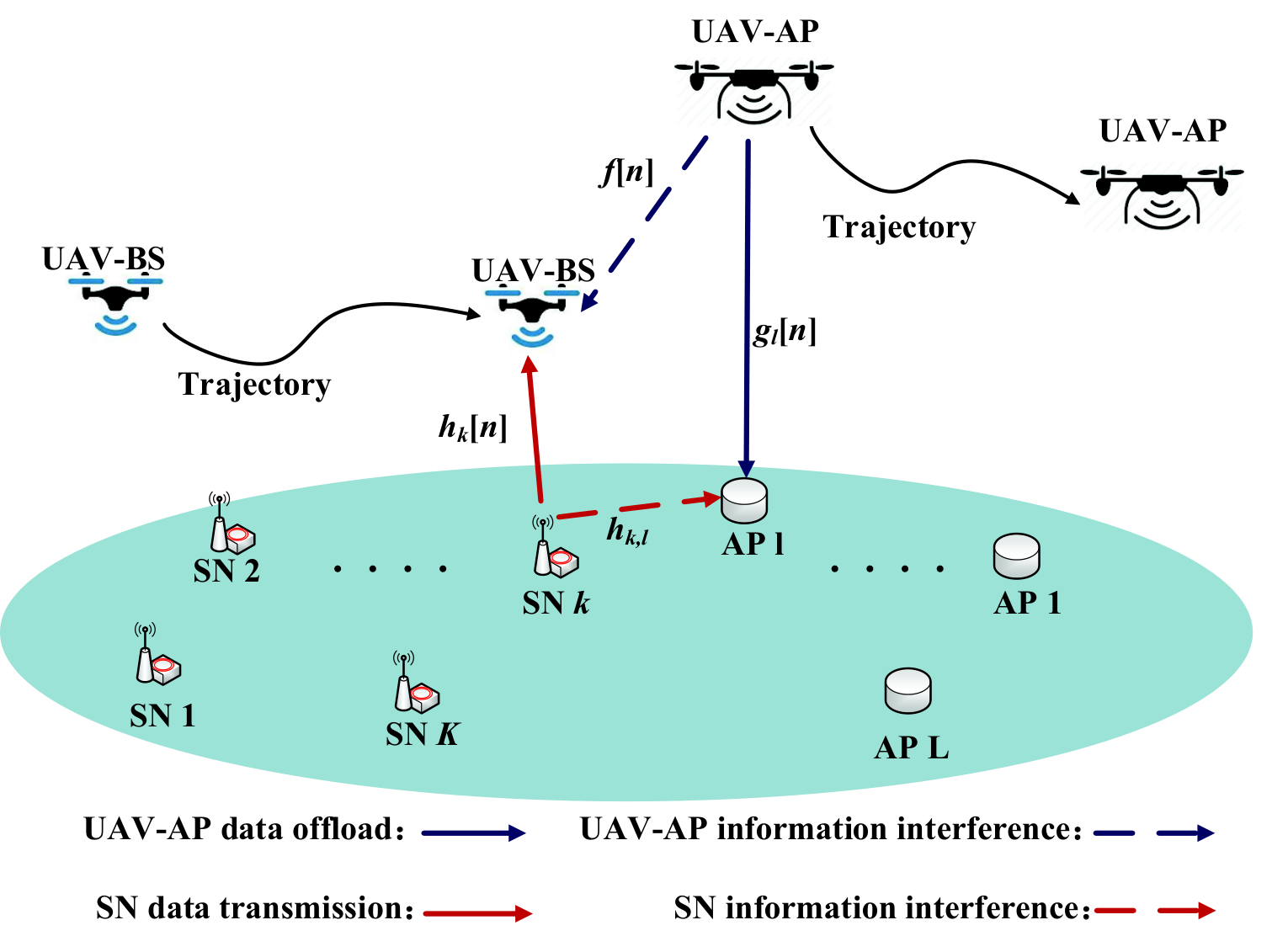
As shown in Fig. 1, several challenges must be addressed in order to achieve good performance for the simultaneous uplink and downlink transmission with the help of UAVs. First, in the UAV-AP based network, namely downlink transmission, the AP not only receives the desired signal from the UAV-AP but also suffers from interference from SNs. Second, in the UAV-BS based network, namely uplink transmission, the UAV-BS not only collects desired data from the SNs but also encounters interference from the UAV-AP. To enhance system performance, the UAV-BS/UAV-AP trajectories must be carefully designed since the UAV location determines its ability to mitigate interference and increase throughput. Furthermore, transmission power of UAV-AP and SN should be jointly optimized to alleviate the whole system interference. Note that this work is different from [31], where a single full-duplex UAV is used to transmit data to the downlink users and receive data from the uplink users simultaneously via a $2\rm D$ trajectory design. However, self-interference and multiple access delay issues impede its application for the single full-duplex UAV used in delay-sensitive tasks. In this paper, we consider multiple half-duplex UAVs to simultaneously serve downlink users and uplink users, the optimization of altitude and transmission power of UAVs resulting in a heterogeneous networks, which provides additional degrees of freedom for achieving low delay and ultra-reliable communications via a $3\rm D$ trajectory design. In addition, we propose a novel method to address the resulting problem, and a globally optimal solution is obtained here. It is worth pointing out that work [29] only focuses the case of multiple UAVs serving multiple users in downlink transmission, whereas the uplink transmission is not considered. To the best of our knowledge, this work is first to study simultaneous uplink and downlink transmission with help of multiple UAVs. Our main contributions are summarized as follows.

• •

  We investigate the scenario of simultaneous uplink and downlink transmission with help of multiple UAVs. We focus on maximizing the sum of the UAV-BS and UAV-AP based network throughput subject to the constraints of UAV mobility and SN/UAV-AP transmit power.

• •

  We first study the case that the UAV-BS and UAV-AP trajectories are pre-determined. We aim at maximizing the sum system throughput by jointly optimizing the SN/UAV-AP transmit power and communication scheduling. The resulting optimization problem is a non-convex integer optimization problem, whose solution is difficult to obtain. However, by exploiting the hidden monotonic nature of the problem, we find a globally optimal solution using the polyblock outer approximation (POA) method. Note that although [28] obtains a globally optimal solution to solar-powered UAV systems using POA method, it only focuses on a single UAV in the downlink transmission, we extend it to a more general case with multiple UAVs in the simultaneous uplink and downlink transmission. In addition, we also propose a suboptimal solution based on the successive convex approximation (SCA) technique. Our numerical results show that the SCA-based method can achieve nearly the same system performance as the POA-based method but with much lower computational complexity.

• •

  We then study a more general scenario in which the UAV-BS and UAV-AP trajectories are optimized. Our goal is to maximize the sum system throughput by jointly designing the UAV-BS/UAV-AP trajectories, SN/UAV-AP transmit power, and communication scheduling. The resulting optimization problem is much more challenging to solve. Nevertheless, we decompose the problem into three sub-problems: communication scheduling with fixed transmit power and UAV trajectory sub-problem, UAV trajectory with fixed transmit power and communication scheduling sub-problem, and transmit power with fixed UAV trajectory and communication scheduling sub-problem. A three-layer iterative algorithm is then proposed to alternately optimize the communication scheduling, UAV trajectory, and transmit power based on the SCA method.

• •

  To demonstrate our designs more clearly, we consider two simulation scenarios. In the first scenario, one UAV-BS collects data from one SN and one UAV-AP transmits its own data to one AP. In the second scenario, the UAV-BS and UAV-AP simultaneously serve multiple SNs and APs. The impact of the weighting factors, UAV trajectory, and transmit power on the system performance are also studied to reveal useful insights. Numerical results show that our proposed scheme achieves significantly higher system throughput compared with other benchmarks.

The rest of the paper is organized as follows. In Section II, we introduce our system model and formulate the system throughput maximization problem. Section III studies the optimal communication design problem. Section IV investigates the joint 3D UAV trajectory and communication design problem. In Section V, numerical results are presented to illustrate the superiority of our scheme. Finally, Section VI concludes the paper.

We consider an integrated network which consists of a UAV-AP and a UAV-BS based network, as shown in Fig. 1. Without loss of generality, we assume that there are $K$ SNs and $L$ APs, which are in fixed locations. The SN and AP sets are respectively denoted as $\cal K$ and $\cal L$. The horizontal coordinates of the $k$th SN and $l$th AP are respectively denoted as ${\bf w}_{bk},k\in\cal K$ and ${\bf w}_{ul},l\in\cal L$. We assume that the UAVs can adjust their heading as needed. The period $T$ is equally divided into $N$ time slots indexed by $n=1,...,N$, with duration $\delta$, i.e., $\delta=\frac{T}{N}$. Note that the duration $\delta$ should be chosen to be sufficiently small so that the UAV’s location can be considered unchanged within each time slot even at the maximum flying speed. As a result, the 3D UAV-AP location at any time slot $n$ is denoted by ${{\bf{w}}_{u}}\left[n\right]=\left[{{{\bf q}_{u}}\left[n\right]{\kern 1.0pt}{\kern 1.0pt}{\kern 1.0pt}{\kern 1.0pt}{H_{u}}\left[n\right]}\right]$, where ${\bf q}_{u}[n]$ and $H_{u}[n]$ denote the horizontal UAV-AP location and altitude, respectively. Similarly, the 3D UAV-BS location at any time slot $n$ is denoted by ${{\bf{w}}_{b}}\left[n\right]=\left[{{{\bf{q}}_{b}}\left[n\right]{\kern 1.0pt}{\kern 1.0pt}{\kern 1.0pt}{\kern 1.0pt}{H_{b}}\left[n\right]}\right]$, where ${\bf q}_{b}[n]$ and $H_{u}[n]$ denote the horizontal UAV-BS location and altitude, respectively.

For the UAV-to-ground (U2G) channel, ground-to-UAV (G2U) channel, and UAV-to-UAV (U2U) channel, the UAV is likely to establish LoS links for all U2G, G2U, and U2U channels as reported in [11], [32]. To capture the large-scale fading as well as small-scale fading, we model the U2G, G2U, and U2U channels as Rician models [14], [27], [33]¹¹ 1 Although Nakagmi-m also captures the LoS propagation [34], it is so sophisticated for analysis in our considered scenarios. To facilitate the system design, we consider a Rician fading model which is relative simple but still appealing in practice. Thus, the U2G channel coefficient, i.e., UAV-AP to AP $l$, $\forall l$, at time slot $n$ can be expressed as

where ${{\beta_{a,l}}\left[n\right]}$ represents its distance-dependent path-loss at time slot $n$, and ${\hat{g}_{l}}\left[n\right]$ is a complex-valued random variable that denotes the small-scale fading at time slot $n$. Specifically, ${{\beta_{a,l}}\left[n\right]}$ can be written as

where $\beta_{0}$ denotes the channel power gain at the reference distance of 1 meter, and $\kappa_{a}$ denotes the U2G path loss exponent. The small-scale fading, ${{\hat{g}}_{l}}\left[n\right]$, can be modeled as below

where ${{\tilde{g}}_{l}}\left[n\right]$ denotes the deterministic LoS channel component with $\left|{{{\tilde{g}}_{l}}\left[n\right]}\right|=1$, ${{\tilde{\tilde{g}}}_{l}}\left[n\right]\sim{\cal CN}\left({0,1}\right)$ denotes the small fading coefficient, and ${{K_{a}}}$ is the Rician factor for the U2G channel.

Similarly, the channel coefficient from SN $k$ to UAV-BS at time slot $n$ can be expressed as

where ${\beta_{s,k}}\left[n\right]={{{\beta_{0}}}\over{{{\left({{{\left\|{{{\bf{q}}_{b}}\left[n\right]-{{\bf{w}}_{bk}}}\right\|}^{2}}+H_{b}^{2}\left[n\right]}\right)}^{{{{\kappa_{s}}}\mathord{\left/{\vphantom{{{\kappa_{s}}}2}}\right.\kern-1.2pt}2}}}}}$, ${{\hat{h}}_{k}}\left[n\right]=\sqrt{{{{K_{s}}}\over{{K_{s}}+1}}}{{\tilde{h}}_{k}}\left[n\right]+\sqrt{{1\over{{K_{s}}+1}}}{{\tilde{\tilde{h}}}_{k}}\left[n\right]$, $\left|{{{\tilde{h}}_{k}}\left[n\right]}\right|=1$, ${{\tilde{\tilde{h}}}_{k}}\left[n\right]\sim{\cal CN}\left({0,1}\right)$, and $\kappa_{s}$ and $K_{s}$ denote the G2U path loss exponent and Rician factor, respectively.

Furthermore, the channel coefficient for the U2U channel, i.e., UAV-AP to UAV-BS channel, is given by

where ${\beta_{u}}\left[n\right]={{{\beta_{0}}}\over{{{\left({\left\|{{{\bf{w}}_{u}}\left[n\right]-{{\bf{w}}_{b}}\left[n\right]}\right\|}\right)}^{{{{\kappa_{u}}}\mathord{\left/{\vphantom{{{\kappa_{u}}}2}}\right.\kern-1.2pt}2}}}}}$, ${{\hat{f}}}\left[n\right]=\sqrt{{{{K_{u}}}\over{{K_{u}}+1}}}{{\tilde{f}}}\left[n\right]+\sqrt{{1\over{{K_{u}}+1}}}{{\tilde{\tilde{f}}}}\left[n\right]$, and $\left|{{{\tilde{f}}}\left[n\right]}\right|=1$, ${{\tilde{\tilde{f}}}}\left[n\right]\sim{\cal CN}\left({0,1}\right)$, and $\kappa_{u}$ and $K_{u}$ denote the U2U path loss exponent and Rician factor, respectively.

Note that the path loss exponents for all the channels depend on the environment. For example, it was shown in [35] that the path loss exponents for U2G/G2U and U2U are $2.32$/$2.51$ and $2.05$, respectively, and the results in [36] shown that the path loss exponents for U2G and U2U are $2.13$ and $1.92$, respectively. Therefore, in the sequel, we set path loss exponents as ${\kappa_{a}}={\kappa_{s}}={\kappa_{u}}=2$ that are consistent with the most existing works [37, 38, 39, 40, 41]. Although we assume that the path loss exponent is $2$, it can be easily extended to the other cases. In addition, we assume that the Rician factors ${{K_{a}}}$, ${{K_{s}}}$, and ${{K_{u}}}$ are all invariant over time slot $n$ by considering the following reasons. First, since our scenario is considered in the rural and/or suburban district, i.e., clear airspace, the Rician factor thus can be approximately treated to be independent of the varying UAV locations. Second, especially for the long period flying time $T$, the most time for UAV is to stay stationary above the ground nodes, and thus can be considered as invariant at most of the time.

In addition, for the ground-to-ground (G2G) channel, we assume that the G2G channel follows Rayleigh fading due to the rich scattering in the environment. Therefore, the channel coefficient from the $k$th SN to the $l$th AP can be expressed as

where ${{\tilde{h}}_{k,l}}={{{\beta_{0}}}\over{{{\left\|{{{\bf{w}}_{bk}}-{{\bf{w}}_{ul}}}\right\|}^{\alpha}}}}$ stands for the large-scale path loss, $\alpha$ represents the G2G path loss exponent, and ${{\hat{h}}_{k,l}}\sim{\cal CN}\left({0,1}\right)$ denotes the small-scale fading.

To facilitate the system design, we assume the widely used wake-up communication scheduling approach [29],[30], and [40], where the UAV-BS (UAV-AP) can only communicate with at most one SN (AP) in any time slot $n$. Define the indicator variable $y_{k}[n],\forall k,n$ and $x_{l}[n],\forall l,n$ for the UAV-BS and UAV-AP based network, respectively. The UAV-BS serves the $k$th SN if $y_{k}[n]=1$, otherwise, $y_{k}[n]=0$. Similarly, if $x_{l}[n]=1$, the UAV-AP migrates the data to the $l$th AP, and no data is transmitted if $x_{l}[n]=0$. Thus, we have the following scheduling constraints

If the $l$th AP is awakened to communicate with the UAV-AP at time slot $n$, the achievable downlink rate of the $l$th AP is given by

where $p^{u}[n]$ and $p_{k}^{s}[n]$ respectively denote the UAV-AP and $k$th SN transmit power at time slot $n$, and $\sigma^{2}$ represents the noise power at the receiver.

When $y_{k}[n]=1$, the uplink transmission rate of SN $k$ is given by

Obviously, (10) can be simplified as

This is because with (7), if AP $l$ is communicated with UAV-AP at time slot $n$, namely ${x_{l}}\left[n\right]=1$, we have $\sum\nolimits_{l=1}^{L}{{{\left|{{\bar{f}}\left[n\right]}\right|}^{2}}{x_{l}}\left[n\right]{p^{u}}\left[n\right]}={\left|{{\bar{f}}\left[n\right]}\right|^{2}}{p^{u}}\left[n\right]$; if no AP is activated, the transmission power of UAV-AP $p_{u}[n]$ must be zero.

Note that since the channels $\left\{{{{\bar{h}}_{k,l}},{{\bar{h}}_{k}}\left[n\right],{{\bar{g}}_{l}}\left[n\right],\bar{f}\left[n\right]}\right\}$ are the random variables, ${\bar{R}}_{k}^{s}\left[n\right]$ and ${\bar{R}}_{l}^{u}\left[n\right]$ are also the random variables. Additionally, since the probability distribution of ${\bar{R}}_{k}^{s}\left[n\right]$ and ${\bar{R}}_{l}^{u}\left[n\right]$ are challenging to obtain, we are interested in the expected/average achievable rate, defined as $R_{k}^{s}\left[n\right]={\mathbb{E}}\left\{{\bar{R}_{k}^{s}\left[n\right]}\right\}$ and $R_{l}^{u}\left[n\right]={\mathbb{E}}\left\{{\bar{R}_{l}^{u}\left[n\right]}\right\}$. However, the closed-form expressions of $R_{k}^{s}\left[n\right]$ and $R_{l}^{u}\left[n\right]$ are unsolvable due to the difficulty of deriving its probability distribution. To address this issue, we obtain their approximation results based on the following theorem.

In this section, we obtain the globally optimal solution to (15) for the particular case when the two UAV trajectories are pre-determined. In practice, for a large number of UAV applications, the flight paths are fixed, e.g., the UAV flies in a circular path along the cell edge to serve the cell-edge users, or the UAV flies in a straight line to communicate with the ground users [38],[42]. As a result, (15) is simplified as

Problem (16) is difficult to solve due to the coupled power and communication scheduling in (16a) and the binary variables in (15b) and (15c). However, we show how to optimally solve (16) by using monotonic optimization theory [43],[44]. First, it is observed that $y_{k}[n]$ and $x_{l}[n]$ in (16a) can be moved into the numerator of the logarithm terms since $y_{k}[n]=1$ for at most one $k$ ($x_{l}[n]=1$ for at most one $l$). Either way, the terms where $y_{k}[n]=0$ and $x_{l}[n]=0$ do not contribute to the objective valuable. Defining $\tilde{p}_{l}^{u}\left[n\right]={p^{u}}\left[n\right]{x_{l}}\left[n\right]$ for all $l$, $\tilde{p}_{k}^{s}\left[n\right]=p_{k}^{s}\left[n\right]{y_{k}}\left[n\right]$ for all $k$, and $\tilde{P}=\left\{{{{\tilde{p}}^{u}}\left[n\right],\tilde{p}_{k}^{s}\left[n\right],\forall k,n}\right\}$, we formulate the following problem:

where ${\cal{P}}=\left\{{\tilde{P}|0\leq\tilde{p}_{l}^{u}\left[n\right]\leq p_{\max}^{u},0\leq\tilde{p}_{k}^{s}\left[n\right]\leq p_{\max}^{s},\forall k,l,n}\right\}$, and $M$ is a sufficiently large penalty factor.

In this section, we investigate the joint 3D trajectory and communication design optimization for maximizing the system throughput using the low-complexity SCA method. Problem (15) is a mixed integer and non-convex optimization problem due to the objective function (15a), constraints (15b), (15c), and (15k). We decompose problem (15) into three sub-problems, and then optimize each sub-problem in an iterative way. Specifically, the three sub-problems are the communication scheduling optimization with fixed transmit power and 3D UAV trajectory; the 3D UAV trajectory optimization with fixed transmit power and communication scheduling; the transmit power optimization with fixed communication scheduling and 3D UAV trajectory. First, we relax the integer communication scheduling constraints (15b) and (15c) into continuous constraints as

References

- [1] M. Mozaffari, W. Saad, M. Bennis, Y. Nam, and M. Debbah, “A tutorial on UAVs for wireless networks: Applications, challenges, and open problems,” IEEE Commun. Surveys Tuts., vol. 21, no. 3, pp. 2334–2360, 3rd Quat. 2019.
- [2] Y. Zeng, R. Zhang, and T. J. Lim, “Wireless communications with unmanned aerial vehicles: Opportunities and challenges,” IEEE Commun. Mag., vol. 54, no. 5, pp. 36–42, May 2016.
- [3] M. M. Azari, H. Sallouha, A. Chiumento, S. Rajendran, E. Vinogradov, and S. Pollin, “Key technologies and system trade-offs for detection and localization of amateur drones,” IEEE Commun. Mag., no. 1, pp. 51–57, Jan. 2018.
- [4] F. Jiang and A. L. Swindlehurst, “Optimization of UAV heading for the ground-to-air uplink,” IEEE J. Sel. Areas Commun., vol. 30, no. 5, pp. 993–1005, Jun. 2012.
- [5] Z. Han, A. L. Swindlehurst, and K. R. Liu, “Optimization of MANET connectivity via smart deployment/movement of unmanned air vehicles,” IEEE Trans. Veh. Technol., vol. 58, no. 7, pp. 3533–3546, Sept. 2009.
- [6] G. Zhang, Q. Wu, M. Cui, and R. Zhang, “Securing UAV communications via joint trajectory and power control,” IEEE Trans. Wireless Commun., vol. 18, no. 2, pp. 1376–1389, Feb. 2019.
- [7] Q. Wu and R. Zhang, “Common throughput maximization in UAV-enabled OFDMA systems with delay consideration,” IEEE Trans. Commun., vol. 66, no. 12, pp. 6614–6627, Dec. 2018.
- [8] Q. Song, F.-C. Zheng, Y. Zeng, and J. Zhang, “Joint beamforming and power allocation for UAV-enabled full-duplex relay,” IEEE Trans. Veh. Technol., vol. 68, no. 2, pp. 1657–1671, Feb. 2018.
- [9] X. Li, H. Yao, J. Wang, X. Xu, C. Jiang, and L. Hanzo, “A near-optimal UAV-aided radio coverage strategy for dense urban areas,” IEEE Trans. Veh. Technol., vol. 68, no. 9, pp. 9098–9109, Sept. 2019.
- [10] X. Zhou, Q. Wu, S. Yan, F. Shu, and J. Li, “UAV-enabled secure communications: Joint trajectory and transmit power optimization,” IEEE Trans. Veh. Technol., vol. 68, no. 4, pp. 4069–4073, Apr. 2019.
- [11] Y. Zeng, Q. Wu, and R. Zhang, “Accessing from the sky: A tutorial on UAV communications for 5G and beyond,” Proc. IEEE, vol. 107, no. 12, pp. 2327–2375, Dec. 2019.
- [12] I. Jawhar, N. Mohamed, J. Al-Jaroodi, and S. Zhang, “A framework for using unmanned aerial vehicles for data collection in linear wireless sensor networks,” J. Intell. Robot. Syst., vol. 74, no. 1-2, pp. 437–453, Apr. 2014.
- [13] M. Dong, K. Ota, M. Lin, Z. Tang, S. Du, and H. Zhu, “UAV-assisted data gathering in wireless sensor networks,” J. Supercomput., vol. 70, no. 3, pp. 1142–1155, Apr. 2014.
- [14] C. Zhan, Y. Zeng, and R. Zhang, “Energy-efficient data collection in UAV enabled wireless sensor network,” IEEE Wireless Commun. Lett., vol. 7, no. 3, pp. 328–331, Jun. 2018.
- [15] Y. Zeng, J. Lyu, and R. Zhang, “Cellular-connected UAV: Potential, challenges, and promising technologies,” IEEE Wireless Commun., vol. 26, no. 1, pp. 120–127, Feb. 2018.
- [16] S. Zhang, Y. Zeng, and R. Zhang, “Cellular-enabled UAV communication: A connectivity-constrained trajectory optimization perspective,” IEEE Trans. Commun., vol. 67, no. 3, pp. 2580–2604, Mar. 2018.
- [17] S. Zhang, H. Zhang, B. Di, and L. Song, “Cellular UAV-to-X communications: Design and optimization for multi-UAV networks,” IEEE Trans. Wireless Commun., vol. 18, no. 2, pp. 1346–1359, Feb. 2019.
- [18] A. Fotouhi, H. Qiang, M. Ding, M. Hassan, L. G. Giordano, A. Garcia-Rodriguez, and J. Yuan, “Survey on UAV cellular communications: Practical aspects, standardization advancements, regulation, and security challenges,” IEEE Commun. Surveys Tuts., vol. 21, no. 4, pp. 3417–3442, 4th Quat. 2019.
- [19] M. M. Azari, F. Rosas, and S. Pollin, “Cellular connectivity for UAVs: Network modeling, performance analysis, and design guidelines,” IEEE Trans. Wireless Commun., vol. 18, no. 7, pp. 3366–3381, Jul. 2019.
- [20] M. Alzenad, A. El-Keyi, and H. Yanikomeroglu, “3-D placement of an unmanned aerial vehicle base station for maximum coverage of users with different QoS requirements,” IEEE Wireless Commun. Lett., vol. 7, no. 1, pp. 38–41, Feb. 2017.
- [21] A. Al-Hourani, S. Kandeepan, and S. Lardner, “Optimal LAP altitude for maximum coverage,” IEEE Wireless Commun. Lett., vol. 3, no. 6, pp. 569–572, Dec. 2014.
- [22] M. M. Azari, F. Rosas, K. Chen, and S. Pollin, “Ultra reliable UAV communication using altitude and cooperation diversity,” IEEE Trans. Commun., vol. 66, no. 1, pp. 330–344, Jan. 2018.
- [23] M. Mozaffari, W. Saad, M. Bennis, and M. Debbah, “Efficient deployment of multiple unmanned aerial vehicles for optimal wireless coverage,” IEEE Commun. Lett., vol. 20, no. 8, pp. 1647–1650, Aug. 2016.
- [24] J. Wang, C. Jiang, Z. Wei, C. Pan, H. Zhang, and Y. Ren, “Joint UAV hovering altitude and power control for space-air-ground IoT networks,” IEEE Internet of Things J., vol. 6, no. 2, pp. 1741–1753, Apr. 2018.
- [25] H. Dai, H. Zhang, M. Hua, C. Li, Y. Huang, and B. Wang, “How to deploy multiple uavs for providing communication service in an unknown region?” IEEE Wireless Commun. Lett., vol. 8, no. 4, pp. 1276–1279, Aug. 2019.
- [26] Y. Zeng and R. Zhang, “Energy-efficient UAV communication with trajectory optimization,” IEEE Trans. Wireless Commun., vol. 16, no. 6, pp. 3747–3760, Jun. 2017.
- [27] C. You and R. Zhang, “3D trajectory optimization in Rician fading for UAV-enabled data harvesting,” IEEE Trans. Wireless Commun., vol. 18, no. 6, pp. 3192–3207, Jun. 2019.
- [28] Y. Sun, D. Xu, D. W. K. Ng, L. Dai, and R. Schober, “Optimal 3D-trajectory design and resource allocation for solar-powered UAV communication systems,” IEEE Trans. Commun., vol. 67, no. 6, pp. 4281–4298, Jun. 2019.
- [29] Q. Wu, Y. Zeng, and R. Zhang, “Joint trajectory and communication design for multi-UAV enabled wireless networks,” IEEE Trans. Wireless Commun., vol. 17, no. 3, pp. 2109–2121, Mar. 2018.
- [30] M. Hua, Y. Wang, Q. Wu, H. Dai, Y. Huang, and L. Yang, “Energy-efficient cooperative secure transmission in multi-UAV-enabled wireless networks,” IEEE Trans. Veh. Technol., vol. 68, no. 8, pp. 7761–7775, Aug. 2019.
- [31] M. Hua, L. Yang, C. Pan, and A. Nallanathan, “Throughput maximization for full-duplex UAV aided small cell wireless systems,” IEEE Wireless Commun. Lett., vol. 9, no. 4, pp. 475–479, Apr. 2020.
- [32] A. A. Khuwaja, Y. Chen, N. Zhao, M. Alouini, and P. Dobbins, “A survey of channel modeling for UAV communications,” IEEE Commun. Surveys Tuts., vol. 20, no. 4, pp. 2804–2821, 4th Quat. 2018.
- [33] C. Zhan and Y. Zeng, “Aerial-ground cost tradeoff for multi-UAV-enabled data collection in wireless sensor networks,” IEEE Trans. Commun., vol. 68, no. 3, pp. 1937–1950, Mar. 2020.
- [34] M. M. Azari, G. Geraci, A. Garcia-Rodriguez, and S. Pollin, “UAV-to-UAV communications in cellular networks,” 2019. [Online]. Available: https://arxiv.org/abs/1912.07534
- [35] N. Ahmed, S. S. Kanhere, and S. Jha, “On the importance of link characterization for aerial wireless sensor networks,” IEEE Commun. Mag., vol. 54, no. 5, pp. 52–57, May 2016.
- [36] J. Allred, A. B. Hasan, S. Panichsakul, W. Pisano, and K. Mohseni, “Sensorflock: an airborne wireless sensor network of micro-air vehicles,” in Proc. SenSys, Nov. 2007, pp. 1937–1950.
- [37] J. Xu, Y. Zeng, and R. Zhang, “UAV-enabled wireless power transfer: Trajectory design and energy optimization,” IEEE Trans. Wireless Commun., vol. 17, no. 8, pp. 5092–5106, Aug. 2018.
- [38] J. Lyu, Y. Zeng, and R. Zhang, “UAV-aided offloading for cellular hotspot,” IEEE Trans. Wireless Commun., vol. 17, no. 6, pp. 3988–4001, Jun. 2018.
- [39] F. Zhou, Y. Wu, R. Q. Hu, and Y. Qian, “Computation rate maximization in UAV-enabled wireless-powered mobile-edge computing systems,” IEEE J. Sel. Areas Commun., vol. 36, no. 9, pp. 1927–1941, Sep. 2018.
- [40] M. Hua, Y. Wang, Z. Zhang, C. Li, Y. Huang, and L. Yang, “Power-efficient communication in UAV-aided wireless sensor networks,” IEEE Commun. Lett., vol. 22, no. 6, pp. 1264–1267, Jun. 2018.
- [41] Q. Wu, J. Xu, and R. Zhang, “Capacity characterization of UAV-enabled two-user broadcast channel,” IEEE J. Sel. Areas Commun., vol. 36, no. 9, pp. 1955–1971, Sep. 2018.
- [42] J. Lyu, Y. Zeng, and R. Zhang, “Cyclical multiple access in UAV-aided communications: A throughput-delay tradeoff,” IEEE Wireless Commun. Lett., vol. 5, no. 6, pp. 600–603, Dec. 2016.
- [43] H. Tuy, “Monotonic optimization: Problems and solution approaches,” SIAM J. Optimiz, vol. 11, no. 2, pp. 464–494, Feb. 2000.
- [44] Y. J. A. Zhang, L. Qian, J. Huang et al., “Monotonic optimization in communication and networking systems,” Found Trends Netw., vol. 7, no. 1, pp. 1–75, Oct. 2013.
- [45] A. Zappone, E. Björnson, L. Sanguinetti, and E. Jorswieck, “Globally optimal energy-efficient power control and receiver design in wireless networks,” IEEE Trans. Signal Process., vol. 65, no. 11, pp. 2844–2859, Jun. 2017.
- [46] S. Boyd and L. Vandenberghe, Convex optimization. Cambridge university press, 2004.
- [47] H. Wang, J. Wang, G. Ding, J. Chen, Y. Li, and Z. Han, “Spectrum sharing planning for full-duplex UAV relaying systems with underlaid D2D communications,” IEEE J. Sel. Areas Commun., vol. 36, no. 9, pp. 1986–1999, Sep. 2018.
- [48] J. Gondzio and T. Terlaky, “A computational view of interior point methods,” JE Beasley. Advances in linear and integer programming. Oxford Lecture Series in Mathematics and its Applications, vol. 4, pp. 103–144, 1996.
![[Uncaptioned image]](2001.00351v2/huameng.png) |
Meng Hua received the M.S. degree in electrical and information engineering from Nanjing University of Science and Technology, Nanjing, China, in 2016. Since September 2016, he is currently working towards the Ph.D. degree in School of Information Science and Engineering, Southeast University, Nanjing, China. His current research interests include UAV assisted communication, intelligent reflecting surface (IRS), backscatter communication, energy-efficient wireless communication, X-connectivity, cognitive radio network, secure transmission, and optimization theory. |
![[Uncaptioned image]](2001.00351v2/Yang.png) |
Luxi Yang (M’96-SM’17) received the M.S. and Ph.D. degrees in electrical engineering from Southeast University, Nanjing, China, in 1990 and 1993, respectively. Since 1993, he has been with the Department of Radio Engineering, Southeast University, where he is currently a Full Professor of information systems and communications, and the Director of the Digital Signal Processing Division. He has authored or co-authored of two published books and more than 200 journal papers, and holds 50 patents. His current research interests include signal processing for wireless communications, MIMO communications, intelligent wireless communications, and statistical signal processing. He received the first and second class prizes of science and technology progress awards of the State Education Ministry of China in 1998, 2002, and 2014. He is currently a member of Signal Processing Committee of the Chinese Institute of Electronics. |
![[Uncaptioned image]](2001.00351v2/Qingqingwu.png) |
Qingqing Wu (S’13-M’16) received the B.Eng. and the Ph.D. degrees in Electronic Engineering from South China University of Technology and Shanghai Jiao Tong University (SJTU) in 2012 and 2016, respectively. He is currently an Assistant Professor in the Department of Electrical and Computer Engineering at the University of Macau, China, and also with the State key laboratory of Internet of Things for Smart City. He was a Research Fellow in the Department of Electrical and Computer Engineering at National University of Singapore. His current research interest includes intelligent reflecting surface (IRS), unmanned aerial vehicle (UAV) communications, and MIMO transceiver design. He has published over 60 IEEE journal and conference papers. He was the recipient of the IEEE WCSP Best Paper Award in 2015, the Outstanding Ph.D. Thesis Funding in SJTU in 2016, the Outstanding Ph.D. Thesis Award of China Institute of Communications in 2017. He was the Exemplary Editor of IEEE Communications Letters in 2019 and the Exemplary Reviewer of several IEEE journals. He serves as an Associate Editor for IEEE Communications Letters and IEEE Open Journal of Communications Society. He is the Lead Guest Editor for IEEE Journal on Selected Areas in Communications on “UAV Communications in 5G and Beyond Networks”, and the Guest Editor for IEEE Open Journal on Vehicular Technology on “6G Intelligent Communications” and IEEE Open Journal of Communications Society on “Reconfigurable Intelligent Surface-Based Communications for 6G Wireless Networks”. He is the workshop co-chair for ICC 2019 and ICC 2020 workshop on “Integrating UAVs into 5G and Beyond”, and the workshop co-chair for GLOBECOM 2020 workshop on “Reconfigurable Intelligent Surfaces for Wireless Communication for Beyond 5G”. |
![[Uncaptioned image]](2001.00351v2/Swindlehurst.png) |
A. Lee Swindlehurst (F’04) received the B.S. (1985) and M.S. (1986) degrees in Electrical Engineering from Brigham Young University (BYU), and the PhD (1991) degree in Electrical Engineering from Stanford University. He was with the Department of Electrical and Computer Engineering at BYU from 1990-2007, where he served as Department Chair from 2003-06. During 1996-97, he held a joint appointment as a visiting scholar at Uppsala University and the Royal Institute of Technology in Sweden. From 2006-07, he was on leave working as Vice President of Research for ArrayComm LLC in San Jose, California. Since 2007 he has been a Professor in the Electrical Engineering and Computer Science Department at the University of California Irvine, where he served as Associate Dean for Research and Graduate Studies in the Samueli School of Engineering from 2013-16. During 2014-17 he was also a Hans Fischer Senior Fellow in the Institute for Advanced Studies at the Technical University of Munich. In 2016, he was elected as a Foreign Member of the Royal Swedish Academy of Engineering Sciences (IVA). His research focuses on array signal processing for radar, wireless communications, and biomedical applications, and he has over 300 publications in these areas. Dr. Swindlehurst is a Fellow of the IEEE and was the inaugural Editor-in-Chief of the IEEE Journal of Selected Topics in Signal Processing. He received the 2000 IEEE W. R. G. Baker Prize Paper Award, the 2006 IEEE Communications Society Stephen O. Rice Prize in the Field of Communication Theory, the 2006 and 2010 IEEE Signal Processing Society’s Best Paper Awards, and the 2017 IEEE Signal Processing Society Donald G. Fink Overview Paper Award. |