![[Uncaptioned image]](2001.00173v1/DOI.png)
|
Phases and excitations of active rod-bead mixtures: simulations and experiments† |
| Harsh Soni,a,b Nitin Kumar,a,c Jyothishraj Nambisan,a,d Rahul Kumar Gupta,b A.K. Sood,a and Sriram Ramaswamya,b | |
![[Uncaptioned image]](2001.00173v1/dates.png)
|
We present a large-scale numerical study, supplemented by experimental observations, of a quasi-two-dimensional active system of polar rods and spherical beads confined between two horizontal plates and energised by vertical vibration. For low rod concentrations we observe a direct phase transition, as bead concentration is increased, from the isotropic phase to a homogeneous flock. For above a threshold value, an ordered band dense in both rods and beads occurs between the disordered phase and the homogeneous flock, in both experiments and simulations. Within the size ranges accessible we observe only a single band, whose width increases with . Deep in the ordered state, we observe broken-symmetry “sound” modes and giant number fluctuations. The direction-dependent sound speeds and the scaling of fluctuations are consistent with the predictions of field theories of flocking, but sound damping rates show departures from such theories. At very high densities we see phase separation into rod-rich and bead-rich regions, both of which move coherently. |
1 Introduction
Active matter is the focus of intense current interest for its dramatic mechanical and statistical properties 1, 2, 3, 4 such as giant number fluctuations 5, 6, 7, 8, wave propagation without conventional inertia 9, 8, 10, 11, broken continuous symmetry in two dimensions, band formation 12, 13, 14, sustained spontaneous oscillations, instability of simple liquid-crystalline order in bulk fluid 15, motile topological defects 6, 7, 16, 17, 18, 19, 20, 21, Motility-Induced Phase Separation and its generalisations 22, 23, 24, 25 and viscosity reduction through internally generated stresses 26, 27, 28. The origin of these properties is the energy supply at the microscopic level, directly to the constituent particles, unlike in conventional nonequilibrium systems such as sheared fluids, which are powered through their periphery. The energy transduction responsible for the active character of a particle could be wholly internal, as in living organisms 29, 30, 31, or it could take place in the region of contact of the particle with its surroundings, as with self-phoretic colloids in a fluid 32, Quincke rollers 33 or vibrated grains 6, 34, 35. Active particles are commonly elongated and can therefore form orientationally ordered states, of which the simplest are nematic and polar uniaxial liquid crystals. Diverse mechanisms underlie the ordering of active particles: in living active systems like bird flocks 36, fish schools and herds the process is behavioural and based on mutual sensing. In active granular systems, which exemplify dry active matter 37, steric and collisional effects give rise to alignment 6, 38. In colloidal rollers a restricted version of the hydrodynamic interaction is responsible 33.
Considerable progress has been made towards understanding active polar systems since the discovery of a flocking phase transition in an agent-based model 39, including field-theoretic arguments towards the existence of long-range order in 2D flocks 40, 8, 3, 41, 11, and predictions of highly anisotropic sound waves – through the interplay of the concentration and broken-symmetry fields – and anomalously large number fluctuations in the ordered phase 9, 8, 3. Recently, Geyer et al. 10 observed sound waves in the suspension of active colloidal rollers. Bertin et al. 42, in a Boltzmann-equation construction of the Toner-Tu equations, discovered that the dependence of the local ordering tendency on the local density inevitably led to a linear instability of the ordered phase, with wavevector parallel to the ordering direction, just past the mean-field flocking transition. Indeed, a banded phase is widely observed to intervene between the isotropic and the uniform ordered phases in agent-based numerical simulations 12, 13, 14 and in experiments on rolling-colloid flocks 33, and arises as well in a variety of theoretical models 43, 44, 45.
Here we study a two-dimensional active polar monolayer consisting of tapered rods adrift in a sea of spherical beads. The energy input to the particles is provided by a vertically vibrated supporting surface, and the rods, by virtue of their shape, transduce this vibration into directed movement in the plane. The spherical beads mediate an aligning interaction between the rods, and otherwise behave like passive particles that move if pushed or dragged by the polar rods. In earlier work on this system 35, 46, 47, we discovered a nonequilibrium phase transition from the isotropic state to an ordered, coherently moving flock, which took place when the concentration of the spherical beads exceeded a critical value which decreased with increasing concentration of rods. Our experimental results were supported by a hydrodynamic theory and numerical simulations incorporating the detailed Newtonian mechanics of the particles and boundaries, including vibration, inelasticity and static friction. In this paper, we offer a a detailed exploration of the phase diagram, mode structure and spatiotemporal correlations of this system, primarily in simulations but supported by key experimental findings. There are of course many parameters one could consider varying, such as the concentrations of rods and beads, the rotational diffusivity of the rods, coefficients of friction between the particles and the substrate, several of which feed into the speed of the rods, and thus mainly change the effective clock speed of the dynamics. We restrict our studies to the dependence on rod area fraction and the bead area fraction . Our numerical studies all employ periodic boundary conditions (PBC) in the horizontal plane, thus eliminating the role of the lateral boundaries of the sample.
Here is a summary of our main results. (i) Large-scale simulation studies over a range of and , with periodic boundary conditions, reveal that a banded state intervenes between the isotropic state and the homogeneous ordered phase, for above a threshold value , as is increased. We see a single coherently moving band rich in both rods and beads, not a periodic array. Detailed studies of band morphology can be found in the body of the paper. Below , the system appears, within our resolution, to undergo a phase transition from a disordered to an ordered state directly, as discussed in 35. (ii) We present experimental evidence for a banded flock, to our knowledge for the first time in dry granular matter. (iii) In the homogeneous ordered state our numerical studies reveal giant number fluctuations and a spectrum of propagating modes. The observed wavevector dependence of the damping rates of the modes differs from the predictions of the Toner-Tu theory, which does however capture other broad features such as the scaling of the number fluctuations, and direction-dependent wavespeeds. (iv) At higher values of total concentration of the rods and the beads we observe phase segregation into bead-rich and aligned rod-rich regions, both moving coherently. The remainder of the paper is organised as follows: in section 2, we discuss our numerical and experimental methods. In section 3 we present our detailed results. We summarise and suggest future directions in the last section 4.
2 Methods
2.1 Experiment
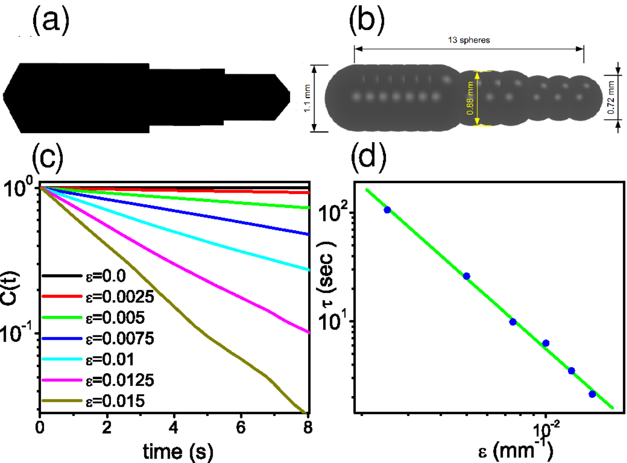
Our experimental cell is a shallow circular geometry, made of hardened aluminium alloy. The particles are confined to two dimensions using a glass lid, which is fixed on the external perimeter of the circle at a height of 1.2 mm above the base. We use the “flower” geometry 48, 35 to prevent clustering of particles on the cell boundary. The cell is mounted on a permanent magnet shaker (LDS 406/8) and is shaken at a fixed frequency and amplitude . The amplitude of the resulting sinusoidal acceleration , measured by an accelerometer (PCB Piezoelectronics 352B02), is chosen to be 7.0 in the units of the gravitational acceleration of the earth . Our “self-propelled” polar particle, which we call a “rod” henceforth, is a brass rod, 4.5 mm long and 1.1 mm in diameter at its thick end as shown in Fig. 1(a). The tilt of the rod with respect to the horizontal transduces the energy of vertical vibration into in-plane propulsion and its geometrical polarity, that is fore-aft asymmetry, ensures that this propulsion is biased towards one end of the rod, specifically, the narrow end. The other particles in our experiment are spherical beads of aluminium, 0.8 mm in diameter, which do not show any in-plane dynamics when vibrated vertically. We created an annular geometry by inserting a circular disk of 5 cm diameter in the middle of the experimental cell. We expected this geometry to stabilize flocking along the azimuthal direction and therefore to favour bands.

2.2 Simulation
Our numerical simulations are based on a mechanically faithful reproduction of the microscopic dynamics of each particle. We assume that all the particles and walls are perfectly rigid. Therefore, all interactions are instantaneous events. All the collisions are inelastic with prescribed restitution and Coulomb friction, and the gravitational acceleration of the earth is taken into account in our simulations. The vibrating base and lid are modelled as horizontal walls moving in the vertical direction with their -coordinates changing with time as and respectively. We do not use the event-driven method 49, often preferred for granular systems at low density, but use instead a time-driven algorithm 50. The latter is more appropriate for our dense system, where an event-driven approach would require a large number of computations to predict the time of the next particle-particle and particle-wall collision 46. Since the rod in experiments has a complicated shape(see Fig. 1a), several calculations are required to detect the collisions between the rods. Therefore, in order to simplify the collision rules and speed up the collision detection process, we construct the rod as an array of overlapping spheres (see Fig. 1b).
The ballistic motion of the particles is governed by Newtonian rigid body dynamics. The Impulse-Based Rigid Body Collision Model 51, 52 is implemented to calculate post collision velocities for all the collisions. We write an MPI-based parallel code to simulate our system: the simulation box is divided into many equal-sized sub-boxes and the dynamics of the particles in different sub-boxes are dealt with by different computer cores. At each step, data for the particles at the boundaries of each sub-box are communicated to the neighbour sub-boxes to execute the collisions between the particles across the sub-boxes. We use VMD software 53 to construct all the simulation movies and snapshots. To achieve the best imitation of the single-particle dynamics of rods and the beads in experiments, we choose the following values of restitution and friction coefficients and :
| Collision | ||
|---|---|---|
| Particle-particle | 0.05 | 0.3 |
| Rod-base(or lid) | 0.03 | 0.1 |
| Rod-boundary | 0.01 | 0.3 |
| Bead-wall(base,lid or boundary) | 0.01 | 0.3 |

We choose the size of the spheres such that the rod in simulations is a close mimic of the original rod in experiments: the tail of the rod is made of seven spheres of mm diameter, and the head and the middle parts each consist of three spheres of diameter mm and mm respectively (see Fig 1b). The beads are represented by spheres of diameter mm. The mass densities of the rods and beads are 8.7 gm/cm3 and 2.7 gm/cm3 corresponding to brass and aluminium respectively. The values of , and are set to 1.2 mm, 200 Hz and 0.04 mm respectively, as in experiments. In experiments, imperfections in shape of the rods and the substrate roughness lead to the diffusive nature of the orientation of the rods. Numerical simulations lack such imperfections. Therefore, we supply the rods with noisy angular velocity in the direction each time they collide with the base or the lid. Here, is the relative velocity at the contact point normal to the contact plane, is a control parameter and with equal probability. Fig 1c shows that the orientation autocorrelation function of a single rod decays exponentially with time , and the relaxation time is decreased with , going as (see Fig. 1d). The value of is set to 0.015, as in 35.
3 Results
We first present our findings from the numerical simulations and then discuss the bands seen in our experiments. In the rest of the paper, all lengths are scaled by the rod length .
3.1 Simulations
The simulations are performed with the periodic box of dimension unless otherwise mentioned. The largest systems we studied had , with 7,200 rods and 300,000 beads. We here discuss the observed phase diagram (see 3.1.1), examine the ordering transition at small (see 3.1.2), study the properties of bands (see 3.1.3), and then present the sound wave spectrum (see 3.1.4) and large density fluctuations (see 3.1.5) in the highly ordered phase.
3.1.1 Phase diagram
Fig. 2a, a phase diagram in the plane of and , gives an overview of the behaviour of the system in various regimes. We mainly observe four phases in our system: disordered, homogeneous ordered, banded, and phase-separated (see Fig 2b-e). The disordered phase, which is found at small values of and , is structureless at very low rod densities (see Fig. 2b) but displays a few randomly moving highly dense and locally ordered swarms at higher values of (see Fig. 11 of Appendix), presumably incomplete MIPS 54, 55. For the band phase is present between the ordered and disordered state (see Fig. 2c). In 3.1.3, we present detailed observations on this phase. Ordered states are observed at higher values of (see Fig. 2d). The velocity field of the bead medium plays an important role in achieving the ordered state 35, as can be seen strikingly through a careful choice of initial conditions. When we perform the simulation of a system which is initially at rest, with the rods in an aligned state, the rods immediately start moving with a constant speed but the beads take some time to pick up their steady state in-plane velocity. Therefore, initially the bead flow is not enough to keep the rods ordered, and the polar order parameter decreases because the rods start disordering. Since they are dragged and pushed by the rods, the beads acquire some speed after some time, and the polar order parameter again increases due to the ordering enhanced by the bead flow (see Fig. 12 of Appendix). More interestingly, the rods can flock at ultra-low (as low as ) if is high enough (see Fig. 13 of Appendix). At very high densities, phase segregation into bead-rich and (ordered) rod-rich regions is observed (see Fig. 2e and Supplementary Movie 1). This regime occurred in our earlier experiments 35, where it was characterised as jamming because the motile rods were immobilised as they pushed up against the sample boundary. A detailed study of the system in this regime will be presented in a separate paper. At higher values of () the rods are condensed into large dense ordered swarms for , through a MIPS-like mechanism (see Fig. 2f).
Finite-size effects are significant in our study. The observed value of and the boundaries of the phases are influenced by system size . We find that decreases as is increased but we find no banded state at even for the system size as big as (or around 457 rod diameters). We do not pursue the question of whether can reach zero for very large systems, as seen in agent based numerical simulations 14.

3.1.2 Phase transition at low
In order to measure the ordering of the rods, we first define the order parameter of the rods as , where is the orientation unit vector of the th rod and denotes the average over all rods and many configurations in the steady state. Our simulations suggest a direct disorder-to-order phase transition without bands at low , although we cannot strictly rule out bands on a much larger length scale. In Fig. 3a we plot the order parameter as a function of for and 0.11.: visibly increases with . In Fig 3b is plotted as the function for , 42, 84 and 112, at . The profile becomes sharper with increasing and the graphs for different don’t intersect with each other, this is consistent with a continuous phase transition, but our size range is limited to conclude. We now calculate the polar order parameter correlation function defined as . Here, the averaging is performed our all the pairs of the rods separated by distance . Fig. 3c, which shows vs for different values of at and L = 112, illustrates that decays to a nonzero constant at high corresponding to the long range ordering, and vanishes for large at low in disordered states 35. Thus, our numerical experiments are consistent with long-range ordering in two dimensions as argued by Toner et al. 40, 41.
3.1.3 Properties of bands
At high rod densities a phase is seen between the order and the disordered states in which a single highly ordered and highly dense stripe of the rods and the beads extended over the length of the simulation box -band- is observed to be moving perpendicular to its own long axis, amidst a disordered background also consisting of of a bead-rod mixture (see Fig. 2e, and Supplementary Movie 2). In this system, up to , the segregation results in a single band unlike the periodically arranged many bands demonstrated by Vicsek particles et al. 12, 14, 56. The bands are generally aligned along the sides of the simulation box but also could be in arbitrary direction at large values of (see Fig. 14 of Appendix). For convenience of analysis we study the regime in which the bands are parallel to the length of the simulation box. Let and be the positions of th rod and th bead respectively, and the velocity of the th bead, at time . Respectively, the coarse grained number densities for the rods and beads are defined as
| (1) | |||
| (2) |
where stands for a sum over all the particles and the integration is taken over a square cell of length centred at position r. Similarly, the polar order parameter field for the rods and the velocity field for the beads are given by
| (3) | |||
| (4) |
In order to quantify the density and ordering profile of the rods we define d and , where we assume that the band is moving along the X axis and the angle bracket represents the average over the direction and time in a frame moving with the band. Similarly, the density profile and the velocity profile of the beads are measured by and . We divide the simulation box into the cells of length one to calculate the value of these functions.

A graphical representation of the bands can be found in Fig. 4a showing the typical density profile of the rods in a band moving in the direction: the scaled density profile of the rods decays faster at the front than at the back i.e. the band is asymmetric with the front sharper than the back. The value of is close to 1 in the band region and fluctuates around 0 elsewhere, and remains close to zero everywhere in the simulation box, indicating that the rods in the band region are aligned along the direction of the motion of the band and randomly oriented elsewhere. An interesting feature of these bands is that even the medium particles, the beads, form bands co-centred with the band of the rods (see Fig. 4b), which is an aspect that cannot arise in the related colloidal rollers 33. In Fig. 4c we plot and as the function of , for and . Again in the band region the average velocity of beads is high and along the direction of the band and vanishingly small elsewhere. Also the profile of is quite similar to of . We further explore the effect of the and total area fraction on the bands. The band becomes wider and denser with increasing at fixed (see Fig. 4d). The condensation of the particles in a single band has also been observed in the active Ising systems 43, 14, but, in contrast, more than one band were observed in Vicsek systems 14 with the number of bands increasing with system size and particle density. The velocity of the bands doesn’t change significantly with but the average velocity of the rods lying in the band region increases, probably because of the suppression of the transverse fluctuations of the orientation of the rods due to the increasing density in the band region (see Fig. 4e). The band moves faster than the rods occupying the band because of the significant velocity gradient at its boundaries. For a given value of , the band widens with increasing , suggesting a tendency to dissolve the band into a homogeneous ordered state at high enough (see Fig. 4f). Correspondingly, goes down with due to enhancement in the transverse fluctuations and rises due to decreasing the density gradient across the band boundaries (see Fig. 4g). A shoulder-like trend is found in vs as a result of the rectangular shape of the bands, indicating the typical width of the band (see Fig. 15 of Appendix). The nature of the phase transition at the boundaries of the segregated regime remains unclear.
Bands in our system do not appear to arise through the instability proposed in 42. Supplementary Movie 2 suggests a different mechanism. Initially small swarms with internal alignment are observed, moving randomly in the isotropic background, with both rods and beads joining and leaving them at their boundary. When the swarms come alongside one another, they unite through lateral exchange of particles to form a band.
In order to explore the possibility of the bands in experiments, we execute the simulations with the annular geometry with outer boundary same as in our experiments 35. Fig. 5 and Supplementary Movie 3 show that the bands should be seen in experiments as well. We will present our experimental result on the bands in subsection 16.
3.1.4 Sound waves
Fig. 2f and Supplementary Movie 4 are evidence for the propagating waves predicted by Toner et al. 8 in the uniform ordered state. In order to measure these waves we calculate the dynamic and static orientation structure factors. Let be the component of the orientation of th rod normal to the direction of the flock. The field for the normal orientation fluctuations is then given by
| (5) |

where sum is taken over all the rods. The static orientation structure factor is defined as
| (6) |
where stands for average over time and
| (7) |
is the Fourier transform of in space. The expression for the dynamic orientation structure factor reads
| (8) |
where angle bracket stands for an average over time or configuration and is the Fourier transform of in time:
| (9) |

In Fig. 6a, vs is reported for modes with wavevectors q parallel and antiparallel to the directions , and with respect to the flocking direction, for , and . We also construct the heat maps for as the function and these three directions (see Fig. 6b): single mode for and two modes for the other cases are clearly visible. Correspondingly, as the function of shows two peaks in all the directions which merge into one along the direction of the flock. The heat map for the static structure factor for orientation is presented in the bottom-right panel of the Fig. 6b, which reveals that the waves are highly anisotropic. Fig. 6c points out that goes as with and along and normal to the flock, respectively. These exponent values are consistent with the Toner-Tu theory 8 which predicts and . The speed of the propagating mode of wave vector q is defined as
| (10) |
where is the position of the peak corresponding to the mode in vs plot. We find that is proportional to for small (see Fig. 7a, b and c for , and respectively), except where is very small, e.g., wavevectors at to the flocking direction. The width of the peak displays a dependence consistent with a power law . The value of is for , 0.6 and 0.9 for the two peaks at and for both the peaks at (insets of Fig. 7a-c). This is in contrast to the Toner-Tu 8 prediction and . Fig. 7d shows the angular dependence of at . Two loops intersecting at correspond to two wave modes. All these observations fairly agree with the theoretical predictions 8 except the wavenumber dependence of the sound peak widths. These waves have been already detected in the numerical simulations of Vicsek-style models 9 but observing them in our numerical model, which is mechanically realistic rather than agent-based, suggests that these modes should exist in real granular-matter experiments. For a systematic evaluation of the Toner-Tu predictions against large-scale numerical studies of the Vicsek model see 57.
3.1.5 Large density fluctuations

In the thermal equilibrium systems away from critical points, in the thermodynamic limit, the particle number fluctuations in the grand canonical ensemble grow as the square root of the average number of the particle as the system size is increased i.e. root-mean-square deviation
| (11) |
where is the instantaneous number of the particles and represents the ensemble average for a given system size. In contrast, active systems show anomalous number fluctuation properties: hydrodynamical theories 8, 15, 5 suggest that for active polar and apolar systems is proportional to in isotropic states but the broken-symmetry states demonstrate large number fluctuations growing as 8, 15, 5
| (12) |
where in mean field theory and has smaller values in renormalization-group treatments of active polar 8 and nematic 58 phases. We construct series of the number of the particles inside the subsystems of different sizes co-centred with the original system, from many statistically independent realizations. We then calculate and for each subsystems. At low , in the disordered isotropic state, is proportional to (see Fig. 8a for and ). Fig. 8a presents vs for three different ordered states: the number fluctuations are larger than the thermal systems with but weaker than the ones predicted by Toner-Tu theory. More detailed studies with finite-size scaling are required for a definitive exponent estimate. Here we should make it clear that the large number fluctuations in order states are not due to a segregation as seen in Fig. 2e & h: a typical ordered state has homogenous rod density (see Fig. 8b).
In order to quantify the lifetime of the number fluctuations we also calculate the density autocorrelation function defined as
| (13) |
where is the average density at the position r and represent the average over space. The coarse-grained number density for the rods has been defined in 3.1.3.Fig. 9 suggests that shows two exponential decays. We do not understand this observation. A linearized treatment as in Narayan et al. 6 would give a logarithmic decay, while the Toner-Tu theory 8 would give a slower in two dimensions. Neither of these forms gives a reasonable fit to our data.

3.2 Experiments

As we showed in earlier work 35, a flocking transition can be triggered at very low area fraction of motile polar rods by increasing the concentration of non-motile beads (see Fig. 16 of Appendix). Here, motivated by our simulations, we perform the experiments in annular geometry at varying and and find that for parameter values shortly past onset of flocking a band does emerge, with appearance typically as in Fig. 10b-f and Supplementary Movie 5. The band is identified as the area of high density of rods and beads with high degree of orientational order which is moving in the direction of its order, with a background of isotropic mixture with low concentration of both rods and beads. Fig. 10 indicates that, at fixed , the band becomes wider as increased, which is consistent with our simulation results. The location of the bands in the plane is depicted in the phase diagram in Fig. 2a. Although the observation of band formation in our experiments is robust, limitations on system size make a more systematic study impractical.
4 Future directions and summary
The research presented in this article was motivated by multiple aims. One was to study collective motion with both self-propulsion and alignment arising for purely mechanical rather than behavioural reasons. The second was to carry out such a study in a system in which – unlike in the Quinke rollers 33 – the strength of interactions could be tuned simply, in this case by changing the bead concentration. Third was to see if the band formation just past ordering onset could be modulated or suppressed. Despite the limitations on system size, we believe we have succeeded in the above aims. Two regimes remain to be explored in more detail. One is the limit of no beads, not discussed here where a patchy MIPS precursor possibly leads to a dilute flock at low noise (see Fig. 17 of Appendix and Supplementary Movie 6). The other is the bead-rod phase separation that occurs at high area fraction of both species.
We close with a summary. In our detailed numerical simulations, we observed four distinct phases of our system: disordered, banded and ordered, homogeneous and ordered, and bead-rod phase separated. The existence of the broken symmetry state at very low rod concentration is a key result. The banded state is similar to the one seen in a system of the polar disks 13 or in the rolling colloids 33: only single bands are observed which are generally aligned with the boundary of the periodic box but also could be in an arbitrary direction at high rod concentration. This is in contrast to the density waves exhibited by the Vicsek model 14. Moreover, in these systems, the band absorbs the bead medium as well, for which there is no equivalent in the other systems like polar disks and colloidal rollers 33. The width of the bands increases with the rod concentration. We also find the first experimental realisation of bands in a dry granular flocking system. We also explore the anisotropic propagating waves and large number fluctuations in the highly ordered state. Some interesting departures are observed with respect to the Toner-Tu theory 8, especially as regards the scaling of damping rate with wavenumber.
Conflicts of interest
There are no conflicts to declare.
Appendix


Acknowledgements
NK, HS and JN thank the UGC, the CSIR and the Science Academies’ Summer Research Fellowship respectively for support. AKS was supported by a Year of Science Professorship by Department of Science and Technology, India and SR by the Tata Education and Development Trust and a J C Bose Fellowship of the SERB.
Notes and references
- Marchetti et al. 2013 M. C. Marchetti, J. F. Joanny, S. Ramaswamy, T. B. Liverpool, J. Prost, M. Rao and R. A. Simha, Rev. Mod. Phys., 2013, 85, 1143–1189.
- Ramaswamy 2010 S. Ramaswamy, Annual Review of Condensed Matter Physics, 2010, 1, 323–345.
- Toner et al. 2005 J. Toner, Y. Tu and S. Ramaswamy, Annals of Physics, 2005, 318, 170 – 244.
- Bechinger et al. 2016 C. Bechinger, R. Di Leonardo, H. Löwen, C. Reichhardt, G. Volpe and G. Volpe, Rev. Mod. Phys., 2016, 88, 045006.
- Ramaswamy et al. 2003 S. Ramaswamy, R. A. Simha and J. Toner, EPL, 2003, 62, 196.
- Narayan et al. 2007 V. Narayan, S. Ramaswamy and N. Menon, Science, 2007, 317, 105–108.
- Narayan 2008 V. Narayan, PhD thesis, Indian Institute of Science, 2008.
- Toner and Tu 1998 J. Toner and Y. Tu, Phys. Rev. E, 1998, 58, 4828–4858.
- Tu et al. 1998 Y. Tu, J. Toner and M. Ulm, Phys. Rev. Lett., 1998, 80, 4819–4822.
- Geyer et al. 2018 D. Geyer, A. Morin and D. Bartolo, Nature materials, 2018, 17, 789.
- Toner 2018 J. Toner, arXiv preprint arXiv:1812.00310, 2018.
- Chaté et al. 2008 H. Chaté, F. Ginelli, G. Grègoire, F. Peruani and F. Raynaud, The European Physical Journal B, 2008, 64, 451–456.
- Weber et al. 2013 C. A. Weber, T. Hanke, J. Deseigne, S. Léonard, O. Dauchot, E. Frey and H. Chaté, Phys. Rev. Lett., 2013, 110, 208001.
- Solon et al. 2015 A. P. Solon, H. Chaté and J. Tailleur, Phys. Rev. Lett., 2015, 114, 068101.
- A. Simha and Ramaswamy 2002 R. A. Simha and S. Ramaswamy, Phys. Rev. Lett., 2002, 89, 058101.
- Sanchez et al. 2012 T. Sanchez, D. T. Chen, S. J. DeCamp, M. Heymann and Z. Dogic, Nature, 2012, 491, 431.
- Giomi et al. 2013 L. Giomi, M. J. Bowick, X. Ma and M. C. Marchetti, Phys. Rev. Lett., 2013, 110, 228101.
- Giomi et al. 2014 L. Giomi, M. J. Bowick, P. Mishra, R. Sknepnek and M. Cristina Marchetti, Philosophical Transactions of the Royal Society A: Mathematical, Physical and Engineering Sciences, 2014, 372, 20130365.
- Shankar et al. 2018 S. Shankar, S. Ramaswamy, M. C. Marchetti and M. J. Bowick, Phys. Rev. Lett., 2018, 121, 108002.
- Doostmohammadi et al. 2018 A. Doostmohammadi, J. Ignés-Mullol, J. M. Yeomans and F. Sagués, Nature communications, 2018, 9, 1–13.
- Kumar et al. 2018 N. Kumar, R. Zhang, J. J. de Pablo and M. L. Gardel, Science advances, 2018, 4, eaat7779.
- Cates and Tailleur 2015 M. E. Cates and J. Tailleur, Annual Review of Condensed Matter Physics, 2015, 6, 219–244.
- Cates 2019 M. Cates, arXiv preprint arXiv:1904.01330, 2019.
- Kumar et al. 2019 N. Kumar, R. K. Gupta, H. Soni, S. Ramaswamy and A. Sood, Physical Review E, 2019, 99, 032605.
- Redner et al. 2013 G. S. Redner, M. F. Hagan and A. Baskaran, Physical review letters, 2013, 110, 055701.
- López et al. 2015 H. M. López, J. Gachelin, C. Douarche, H. Auradou and E. Clément, Phys. Rev. Lett., 2015, 115, 028301.
- Sokolov and Aranson 2009 A. Sokolov and I. S. Aranson, Phys. Rev. Lett., 2009, 103, 148101.
- Ryan et al. 2011 S. D. Ryan, B. M. Haines, L. Berlyand, F. Ziebert and I. S. Aranson, Phys. Rev. E, 2011, 83, 050904.
- Bray 2000 D. Bray, Cell movements: from molecules to motility, Garland Science, 2000.
- Alberts et al. 1994 B. Alberts, D. Bray, J. Lewis, M. Raff, K. Roberts and J. Watson, New York, 1994, 18–19.
- Jülicher et al. 2018 F. Jülicher, S. W. Grill and G. Salbreux, Reports on Progress in Physics, 2018, 81, 076601.
- Saha et al. 2014 S. Saha, R. Golestanian and S. Ramaswamy, Phys. Rev. E, 2014, 89, 062316.
- Bricard et al. 2013 A. Bricard, J.-B. Caussin, N. Desreumaux, O. Dauchot and D. Bartolo, Nature, 2013, 503, 95–98.
- Narayan et al. 2006 V. Narayan, N. Menon and S. Ramaswamy, Journal of Statistical Mechanics: Theory and Experiment, 2006, 2006, P01005.
- Kumar et al. 2014 N. Kumar, H. Soni, S. Ramaswamy and A. Sood, Nature communications, 2014, 5, 4688.
- Cavagna and Giardina 2014 A. Cavagna and I. Giardina, Annu. Rev. Condens. Matter Phys., 2014, 5, 183–207.
- Chaté 2020 H. Chaté, Annual Review of Condensed Matter Physics, 2020, 11, .
- Deseigne et al. 2012 J. Deseigne, S. Leonard, O. Dauchot and H. Chaté, Soft Matter, 2012, 8, 5629–5639.
- Vicsek et al. 1995 T. Vicsek, A. Czirók, E. Ben-Jacob, I. Cohen and O. Shochet, Physical Review Letters, 1995, 75, 1226.
- Toner and Tu 1995 J. Toner and Y. Tu, Phys. Rev. Lett., 1995, 75, 4326–4329.
- Toner 2012 J. Toner, Phys. Rev. Lett., 2012, 108, 088102.
- Bertin et al. 2006 E. Bertin, M. Droz and G. Grégoire, Phys. Rev. E, 2006, 74, 022101.
- Solon and Tailleur 2013 A. P. Solon and J. Tailleur, Phys. Rev. Lett., 2013, 111, 078101.
- Chen and Toner 2013 L. Chen and J. Toner, Phys. Rev. Lett., 2013, 111, 088701.
- Caussin et al. 2014 J.-B. Caussin, A. Solon, A. Peshkov, H. Chaté, T. Dauxois, J. Tailleur, V. Vitelli and D. Bartolo, Phys. Rev. Lett., 2014, 112, 148102.
- Soni 2015 H. Soni, PhD thesis, Indian Institute of Science, 2015.
- Kumar 2015 N. Kumar, PhD thesis, Indian Institute of Science, 2015.
- Deseigne et al. 2010 J. Deseigne, O. Dauchot and H. Chaté, Phys. Rev. Lett., 2010, 105, 098001.
- Pöschel and Schwager 2005 T. Pöschel and T. Schwager, Computational granular dynamics: models and algorithms, Springer Science & Business Media, 2005.
- 50 Understanding Molecular Simulation (Second Edition), ed. D. Frenkel and B. Smit, Academic Press, San Diego, Second Edition edn, 2002, pp. 1 – 661.
- Stronge 1994 W. J. Stronge, Journal of Applied Mechanics, 1994, 61, 605–611.
- Stronge 2000 W. J. Stronge, Impact Mechanics, Cambridge University Press, Cambridge, United Kingdom, 2000.
- Humphrey et al. 1996 W. Humphrey, A. Dalke and K. Schulten, Journal of Molecular Graphics, 1996, 14, 33–38.
- Cates and Tailleur 2015 M. E. Cates and J. Tailleur, Annu. Rev. Condens. Matter Phys., 2015, 6, 219–244.
- 55 In the present context MIPS is simply joint condensation of rods and beads, and should not be confused with the demixing of the two species, which we call segregation, observed at higher area fraction.
- Chaté et al. 2008 H. Chaté, F. Ginelli, G. Grégoire and F. Raynaud, Phys. Rev. E, 2008, 77, 046113.
- Mahault et al. 2019 B. Mahault, F. Ginelli and H. Chaté, Phys. Rev. Lett., 2019, 123, 218001.
- Shankar et al. 2018 S. Shankar, S. Ramaswamy and M. C. Marchetti, Phys. Rev. E, 2018, 97, 012707.