Exact Hyperuniformity Exponents and Entropy Cusps in
Models of Active-Absorbing Transition
Abstract
Recent studies of nonequilibrium phase transitions have shown that in many systems which have transitions involving an arrested phase, the arrested states show suppressed density fluctuations and a cusp in the configurational entropy at the transition point. We study quasistatic driving in the 1D fixed-energy abelian sandpile model, and in conserved lattice gases with range in 1D, and exactly determine the measure over the absorbing states for both cases, along with the behaviour of density fluctuations and the configurational entropy of absorbing states. We show that both models exhibit hyperuniformity near the transition, and also that the configurational entropy shows a cusp at the transition point in the conserved lattice gases.
Introduction Models of active-absorbing phase transitions lubeck2004universal; henkel2008non exhibit a change in the dynamical behaviour of the system from a phase where after a finite time the dynamics is arrested or dies, falling into what are called absorbing states, to a phase where a steady state with finite activity is reached in the thermodynamic limit, as a parameter is varied across the transition point . For , if there are infinitely many absorbing states, the measure over them can depend on the initial conditions. The measurement of near-critical properties in the absorbing phase is thus complicated by the necessity of defining a measure over the absorbing states. The construction of a ‘natural’ measure over absorbing states is an important issue in current debates over the universality class of models with a conserved field basu2012fixed; le2015exact; dickman2015particle. It should be noted that in models of self-organized criticality the presence of an infinitesimal drive and boundary dissipation leads to a unique measure over absorbing states that can, in many cases, be exactly determineddhar1999abelian, and such a measure can exhibit hyperuniformity that is analytically tractable grassberger2016oslo.
In this letter, we study two models with a conserved density that show an active-absorbing phase transition in one dimension. The first model is the abelian sandpile model (ASM), while the second is the class of conserved lattice gases with extended range (CLGs) whose the active steady state behaviour was exactly solved in dandekar2013class. We show that the introduction of a quasistatic drive leads to an exactly solvable measure on the absorbing states in these models. In glassy and jammed systems, such a drive corresponds either to very slow external driving, or to the limit , and is a natural way to study arrested states in these systems radjai2002turbulentlike; howell1999stress; maloney2006amorphous. The external drive we introduce does not break any symmetries of the original dynamics, and allows us to characterize the near critical properties of the absorbing states exactly.
Two interesting characterizations of absorbing or arrested states that have attracted attention in recent years are the hyperuniformity of particle number fluctuations and the configurational entropy.
Translationally invariant arrangements of points in space, or occupied sites on a lattice, can be classified on a scale from regular to random based on the scaling of the number fluctuations in a large probe length scale . For a periodic pattern, the number fluctuations scale as the surface area of the probe volume, . In contrast, when particles are arranged randomly in space, the number fluctuations scale as . In general, if number fluctuations scale as as with between and , the system is said to exhibit hyperuniformityhexner2015hyperuniformity; torquato2016hyperuniformity; torquato2003local; ghosh2017fluctuations. Several studies have found hyperuniformity in jammed packing and athermal structures atkinson2016critical; weijs2015emergent; tjhung2015hyperuniform; gradenigo2015edwards; hexner2018two. Numerical simulations of models of active-absorbing phase transitions with a conserved density have been shown to have hyperuniform fluctuations at the critical point hexner2015hyperuniformity; hexner2017noise. Away from the critical point, hyperuniformity is seen only over a finite length scale, the divergence of which as the critical point is approached defines the hyperuniformity correlation exponent . The exponents and are believed to depend only on the universality class, but so far there are no models for which they can be exactly determined.

Martiniani et al. martiniani2019quantifying measured the behaviour of a measure of configurational entropy, the computable information density (CID), for various active-absorbing phase transitions and found that the behaviour of the entropy of a typical configuration generically shows a cusp at the transition. Other studies since have extended this result to other measures of configurational entropy and more systems avinery2019universal; zu2019information. However, the existence of a cusp has not previously been shown exactly for any model.
We show that for the Abelian Sandpile Model in 1D and Conserved Lattice Gases with extended range, the measure over absorbing states obtained under quasistatic drive exhibits hyperuniformity. We analytically determine the hyperuniformity exponents, and demonstrate exactly the existence of an entropy cusp at the transition point.
1D Conserved Lattice Gases with extended range Conserved Lattice gases are models of particles on the lattice with exclusion interaction, and the property that particles can only move if another particle is present within a specified range. The class of conserved lattice gases we study in this section was defined in dandekar2013class, where the properties of the active steady state were characterised exactly. Consider particles on sites on a 1D ring, such that each site can have no more than 1 particle. The notation denotes a configuration with a contiguous cluster of particles, followed by a contiguous cluster of empty sites, and so on. The allowed transitions for the model with range are (all transitions happen at rate )
| (1) | |||||
For , this is the model known as the Conserved Lattice Gas. It can be seen that for this model, clusters of s of length are transient, since they are not created by the dynamics, and their number reduces monotonically with time. Only for , all transient clusters of s vanish until there are only isolated s in the system, while for , the dynamics eventually enters an absorbing configuration with only isolated s.
In the model with range , if a particle is either right next to another particle, or the total number of s immediately to the left and right is not greater than , the particle is ’active’, and hops to a neighbouring empty site at rate . For the model with range , clusters of s of length are transient. A active steady state exists for , and consists of all configurations with no clusters of length , with equal weight. Using a generating function formalism, the properties of the active steady state were determined in dandekar2013class. Denoting the grand canonical partition function by , where is the fugacity of particles and the fugacity of sites, it was shown that
| (2) | |||||
where is the density of active (moveable) particles at density , and is the correlation length. Hence the critical exponents for the model with range are and .
Transience field We now introduce a field which simulates an external drive, with the limit being equivalent to quasistatic driving. The field is defined by two additional rates
| (3) |
These reactions only apply to isolated particles which cannot move according to the rates in eqns. (1).
It is convenient to think of the transient dynamics of the CLG models as the system going down a ’transience ladder’, with the height of the ladder being the total length of clusters of length . The usual CLG dynamics takes the system down the ladder one step when a hop occurs into one of these clusters, reducing its length by 1. The external field dynamics allows the system to take reverse steps up the ’transience ladder’, at a rate . As , the system settles down on the lowest rung on the transience ladder available at that density. Earlier studies have introduced a field in active-absorbing models which couples to the activity lubeck2002mean; lubeck2002scaling. However, a transience field couples to the position of the system on the transience ladder, and hence is relevant to understanding the nature of the absorbing and transient states.
For any , the dynamics obeys detailed balance, and the equilibrium measure is given by (the s below can be zero)
| (4) |
Defining is the partition function of the system of particles on sites with field , we have the grand canonical partition function,
| (5) |
The grand canonical partition function allows us to analyse the system using methods from generating function theory wilf2005generatingfunctionology, see Appendix A for details. Using the notation , let us denote the largest pole of as . Then, in the thermodynamic limit, a fugacity is equivalent to a density
| (6) |
Hyperuniformity If the initial density is greater than , and we set , the system goes to the active state described in eqn. (2). However, if and we take the limit of quasistatic driving, , the measure concentrates on absorbing states which are on the lowest accessible rung of the transience ladder. These are configurations have, for that and , the minimal number of s in clusters of length , since these have weight or less. Thus the system tries to put as many s as possible into clusters of length , which implies that clusters must be of length or greater. The same effect was seen to arise due to repulsion in the lowest density regime in the generalized repulsion processes studied in krapivsky2013dynamics. The generating function of the measure on the absorbing states is given by
| (7) |
Thus we need to analyse the largest roots of the equation
| (8) |
Now,
| (9) |
The near-critical limit thus corresponds to . The roots of eqn. (8), to order , lie on a circle in the complex plane with the same radius. The largest root is
| (10) |
The roots with the next largest real part are
| (11) |
The correlation length in the system is given in terms of the leading poles of the generating function by
| (12) |
At the critical point, there is only one allowed configuration, , which is periodic. Working slightly below the critical point, one expects that on short lengths , the system will look critical, and hence periodic. At length scales , the different parts of the system are uncorrelated with each other. Thus is precisely the hyperuniformity crossover length.
Similar scaling behaviour of the number fluctuations is expected approaching from the active side as well. As was shown in dandekar2013class, the correlation length in the active state also diverges as . Thus, we have for the conserved lattice gases, for all ranges ,
| (13) |
Entropy cusp at the transition Define the configurational entropy per unit length of a system as
| (14) |
where , where is the microcanonical partition function. The average is over the ensemble with fixed and . As shown in Appendix B, one can write this entropy in terms of largest pole of the grand partition function,
| (15) |
where the energy density of the system. If is the weight of the configuration , is defined as
| (16) |
The second equality follows from the definition of the weights of the CLG, eqn. (4).
In the limit , the system has an equal measure on all allowed states, on both sides of the transition. Thus we can set in eqn. (15). From eqns. (9) and (10), we obtain the entropy of absorbing states slightly below ,
| (17) |
From the generating function for the active steady state, eqn. (2), it was calculated in dandekar2013class that near ,
Giving the entropy of near-critical active states to be
| (18) |
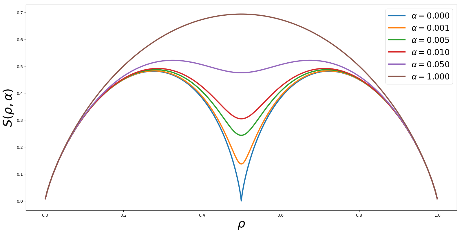
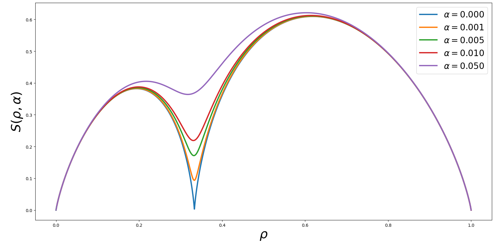
Thus, we see that the entropy goes to on both sides of the transition. At there is only one allowed configuration, , and .
For , we can still obtain parametric equations for , and , which are given in Appendix C. There we also calculate that for at , the entropy is given by
| (19) |
Thus the entropy has a square root cusp along the direction, for all .
The entropy for the and cases is plotted in fig. 2. We see that is non-monotonic in for a given , with a minimum at . The non-monotonicity becomes more pronounced as is decreased, finally developing into the cusp at . Thus, not only does the transience field allow us the analyse the measure over the absorbing states in the quasistatic limit, but even for finite values of the field when there are no absorbing states, we can see that the available phase space shrinks for a certain range of and then increases again. Even though the measure for any finite is an equilibrium measure, it seems the presence of a transience ladder and the incipient active-absorbing phase transition are signalled by this non-monotonicity.
Hyperuniformity in the 1D Abelian Sandpile The Abelian Sandpile model was one of the earliest models discovered to show self-organised criticality in its driven-dissipative versionbak1987self; dhar1999abelian. The version with closed boundaries shows an active-absorbing transition as the total number of particles on the lattice is increased. The transition point is known exactly only for some simple classes of graphs, and can depend on the preparation protocol fey2010driving; fey2010approach. Due to the deterministic nature of the model, the active steady state exhibits several unusual features, such as ergodicity breaking dall2006exact. We study the model below on the 1D ring, where there is no active state.
Consider the ASM with particles on a ring of sites. The number of particles on the site is denoted . If , this site is unstable, and a toppling move occurs (at rate ):
| (20) |
For the ASM, we introduce a quasistatic drive such that for all non-empty sites, one particle jumps from the site to a random neighbour at rate . We refer to this as the ‘ process’. We only work in the quasistatic limit , for , in which case, the process happens only after all sites have stabilised under the ASM rules. However, if the hop takes a particle to an already occupied site, this creates an unstable site, leading to an avalanche of ASM topplings, ending with the system reaching another absorbing state. We now determine the steady-state measure on absorbing configuration induced by the process.
Consider a contiguous cluster of s on the lattice, of length . Say the particle in the cluster moves to the site, due to the process. This makes site unstable, and it topples, transferring one particle to the (now empty) site, and one to the site, making this site unstable in turn. This process continues until the avalanche reaches the right end of the cluster. A toppling at the right end of the cluster results in one particle being thrown out of the cluster to the right, and the cluster length reducing by 1.
Note that the same final state (the cluster length reducing by , one particle thrown out to the right) is reached if any of the particles in the cluster hops to the right. Similarly, if any of the particles in the cluster hops to the left, the clusters throws out a particle to the left. Thus the cluster length reduces by at rate .
Thus the quasistatically driven ASM can be mapped to a zero-range process with out-rates for a site with particles. (To map an ASM absorbing configuration to a ZRP state, the 0’s become sites and the 1-cluster following a 0 becomes the mass on that site.) The steady-state for the ZRP is known exactly, and thus we get the same measure on absorbing configurations for the quasistatically driven ASM:
| (21) |
for a configuration with -clusters of lengths . The grand canonical partition function is given by
| (22) |
We again denote . The largest pole of gives the asymptotic behavior of the canonical partition for sites, for large . As shown in Appendix D, the poles of the generating function are given by
| (23) |
where is the branch of the Lambert function , and is an integer in the range to . The Lambert function veberic2010having is defined though,
| (24) |
which has an infinity of roots in the complex plane, labeled by .
Now, the ASM at has a single absorbing state, , and is trivially periodic. As the transition point at is approached, we expect the correlation length of the system to diverge. The leading pole is given the real branch of eqn. (23), . The next largest roots of the denominator of the generating function are the pair of conjugate roots with . Now, we have for large ,
| (25) |
Since , we have that the correlation length near is
| (26) |
while over shorter distances the system is periodic with a periodicity given the imaginary part . Hence, the hyperuniformity correlation exponent is . As the system is periodic on length scales , we have that the hyperuniformity exponent .
Entropy of Absorbing States Since the distribution of gaps between s, eqn. 21, is a Bernoulli measure, we know that in the grand canonical emsemble this splits into independent Poisson measures for each individual gap. Near , each gap is Poisson-distributed with mean . Thus the total entropy of the system is
| (27) |
where is the number of s in the system, and is the entropy of a Poisson distribution with mean . Although no closed form expression exists for , in the limit of large , it can be written as a series in ,
| (28) |
Hence, we have that,
| (29) |
Thus the entropy goes to at as . A different method for calculating the entropy is given in Appendix E.
Conclusions We have shown that for the class of longer-ranged Conserved Lattice Gases defined in dandekar2013class, and the fixed energy Abelian Sandpile Model in 1D, an exactly calculable measure over the absorbing states can be defined using an external field to induce quasistatic driving. We calculated the hyperuniformity exponents for both cases and showed that the entropy goes to zero as . For the Conserved Lattice Gases, we could calculate the measure exactly even for a finite external field, and showed that the entropy of configurations shows nonmonotonic behaviour around the zero-field transition point, developing into a cusp as the drive is tuned to zero.
The calculation of hyperuniformity in the ASM offers a concrete example of a model where a nontrivial hyperuniformity exponent () can be calculated exactly, and is the first known result of this sort, to our knowledge.
For the CLGs, the non-monotonic behaviour of the entropy even for finite where there are no transient states offers an understanding of the entropy cusp seen in studies of active-absorbing transitions martiniani2019quantifying is not dependent on the exact nature of the measure on the absorbing states (and hence the particular initial conditions employed) but originates simply in the squeezing of the available phase space, seen even in the driven system which has no absorbing states. As the drive is taken to zero, for values before the cusp, this driven measure concentrates on absorbing states, while after the cusp it concentrates on active states. Thus, we believe this allows us to understand active-absorbing phase transitions generically in terms simply of the relative available phase space for absorbing and active states, which switches from being in favour of one to the other at . Since active-absorbing transitions break no symmetries, an thermodynamic understanding of their origin is lacking, and the transience field provides a potential route to the resolution of such an origin.
Acknowledgements I would like to thank Deepak Dhar for suggesting the idea of the slow drive in the ASM, and his constant encouragement and guidance.
References
- [1] Sven Lübeck. Universal scaling behavior of non-equilibrium phase transitions. International Journal of Modern Physics B, 18(31n32):3977–4118, 2004.
- [2] Malte Henkel, Haye Hinrichsen, Sven Lübeck, and Michel Pleimling. Non-equilibrium phase transitions, volume 1. Springer, 2008.
- [3] Mahashweta Basu, Urna Basu, Sourish Bondyopadhyay, PK Mohanty, and Haye Hinrichsen. Fixed-energy sandpiles belong generically to directed percolation. Physical review letters, 109(1):015702, 2012.
- [4] Pierre Le Doussal and Kay Jörg Wiese. Exact mapping of the stochastic field theory for manna sandpiles to interfaces in random media. Physical review letters, 114(11):110601, 2015.
- [5] Ronald Dickman and SD da Cunha. Particle-density fluctuations and universality in the conserved stochastic sandpile. Physical Review E, 92(2):020104, 2015.
- [6] Deepak Dhar. The abelian sandpile and related models. Physica A: Statistical Mechanics and its Applications, 263(1-4):4–25, 1999.
- [7] Peter Grassberger, Deepak Dhar, and PK Mohanty. Oslo model, hyperuniformity, and the quenched edwards-wilkinson model. Physical Review E, 94(4):042314, 2016.
- [8] Rahul Dandekar and Deepak Dhar. A class of exactly solved assisted-hopping models of active-inactive state transition on a line. EPL (Europhysics Letters), 104(2):26003, 2013.
- [9] Farhang Radjai and Stéphane Roux. Turbulentlike fluctuations in quasistatic flow of granular media. Physical review letters, 89(6):064302, 2002.
- [10] Daniel Wyatt Howell. Stress distributions and fluctuations in static and quasi-static granular systems. 1999.
- [11] Craig E Maloney and Anaël Lemaître. Amorphous systems in athermal, quasistatic shear. Physical Review E, 74(1):016118, 2006.
- [12] Daniel Hexner and Dov Levine. Hyperuniformity of critical absorbing states. Physical review letters, 114(11):110602, 2015.
- [13] Salvatore Torquato. Hyperuniformity and its generalizations. Physical Review E, 94(2):022122, 2016.
- [14] Salvatore Torquato and Frank H Stillinger. Local density fluctuations, hyperuniformity, and order metrics. Physical Review E, 68(4):041113, 2003.
- [15] Subhroshekhar Ghosh and Joel L Lebowitz. Fluctuations, large deviations and rigidity in hyperuniform systems: a brief survey. Indian Journal of Pure and Applied Mathematics, 48(4):609–631, 2017.
- [16] Steven Atkinson, Ge Zhang, Adam B Hopkins, and Salvatore Torquato. Critical slowing down and hyperuniformity on approach to jamming. Physical Review E, 94(1):012902, 2016.
- [17] Joost H Weijs, Raphaël Jeanneret, Rémi Dreyfus, and Denis Bartolo. Emergent hyperuniformity in periodically driven emulsions. Physical review letters, 115(10):108301, 2015.
- [18] Elsen Tjhung and Ludovic Berthier. Hyperuniform density fluctuations and diverging dynamic correlations in periodically driven colloidal suspensions. Physical review letters, 114(14):148301, 2015.
- [19] Giacomo Gradenigo, Ezequiel E Ferrero, Eric Bertin, and Jean-Louis Barrat. Edwards thermodynamics for a driven athermal system with dry friction. Physical review letters, 115(14):140601, 2015.
- [20] Daniel Hexner, Andrea J Liu, and Sidney R Nagel. Two diverging length scales in the structure of jammed packings. Physical review letters, 121(11):115501, 2018.
- [21] Daniel Hexner and Dov Levine. Noise, diffusion, and hyperuniformity. Physical review letters, 118(2):020601, 2017.
- [22] Stefano Martiniani, Paul M Chaikin, and Dov Levine. Quantifying hidden order out of equilibrium. Physical Review X, 9(1):011031, 2019.
- [23] Ram Avinery, Micha Kornreich, and Roy Beck. Universal and accessible entropy estimation using a compression algorithm. Physical review letters, 123(17):178102, 2019.
- [24] Mengjie Zu, Arunkumar Bupathy, Daan Frenkel, and Srikanth Sastry. Information density, structure and entropy in equilibrium and non-equilibrium systems. arXiv preprint arXiv:1912.03876, 2019.
- [25] S Lübeck and A Hucht. The mean-field scaling function of the universality class of absorbing phase transitions with a conserved field. Journal of Physics A: Mathematical and General, 35(23):4853, 2002.
- [26] S Lübeck. Scaling behavior of the order parameter and its conjugated field in an absorbing phase transition around the upper critical dimension. Physical Review E, 65(4):046150, 2002.
- [27] Herbert S Wilf. generatingfunctionology. AK Peters/CRC Press, 2005.
- [28] PL Krapivsky. Dynamics of repulsion processes. Journal of Statistical Mechanics: Theory and Experiment, 2013(06):P06012, 2013.
- [29] Per Bak, Chao Tang, and Kurt Wiesenfeld. Self-organized criticality: An explanation of the 1/f noise. Physical review letters, 59(4):381, 1987.
- [30] Anne Fey, Lionel Levine, and David B Wilson. Driving sandpiles to criticality and beyond. Physical review letters, 104(14):145703, 2010.
- [31] Anne Fey, Lionel Levine, and David B Wilson. Approach to criticality in sandpiles. Physical Review E, 82(3):031121, 2010.
- [32] Luca Dall’Asta. Exact solution of the one-dimensional deterministic fixed-energy sandpile. Physical review letters, 96(5):058003, 2006.
- [33] Darko Veberic. Having fun with lambert w (x) function. arXiv preprint arXiv:1003.1628, 2010.
Appendix A The grand canonical partition function
The microcanonical partition function is defined as the sum of the weights of all configurations on a ring of sites, with particles, with denoting the number of particles on site in configuration ,
| (30) |
For a lattice of sites we set by definition. The canonical partition function, is defined for a lattice of fixed size , while the number of particles is allowed to vary:
| (31) |
The grand canonical partition is defined as
| (32) |
Let us suppose that the weights break up into products of weights of subconfigurations, as happens for the models studied in this paper. Consider the minimal set of subconfigurations needed to define the weights in this fashions. This implies that every given configuration can be formed from the minimal set in a unique way. For example, in the conserved lattice gas with and , the minimal set is simply and . Denote the minimal set of subconfigurations by , and let and denote the number of particles and length respectively of subconfiguration . We define
| (33) |
By using the fact that the configurations summed over in are sequences of all allowed subconfigurations with the correct weights, one has
| (34) |
where depends only on the boundary condition. Consider the poles of , which are the roots of ,
| (35) |
Then,
| (36) |
For convenience of notation we denote as , and this implies
| (37) |
Let . Then, we have
| (38) |
And the subleading correction to this ‘free energy’ is
| (39) |
where is the largest correlation length in the system, and which is thus given by
| (40) |
Appendix B Configurational Entropy from the partition function
The canonical partition function can be written as
| (41) |
Changing variables to and , converting the sum to an integral, and using a saddle point approximation, and the typical value of in the system is
| (42) |
If the saddle-point approximation is valid, is also the mean density of the system with fugacity ,
| (43) |
Taking logarithms of both sides of eqn. (41),
| (44) |
Now, for a system with fixed and , the probabilities of various configurations are given as . The configurational entropy is
| (45) |
Defining the energy density , and the entropy density , we have
| (46) |
Therefore, we have
| (47) |
Appendix C Parametric expressions for , and for the CLG for general and
| (48) | |||||
| (49) | |||||
| (50) |
To get the behaviour of at the critical point, we set in the first equation and solve for . Expanding this for (which is the correct limit near the critical point), as for , at in the active steady state [8]), we get
Appendix D Poles of the generating function for the 1D ASM
The grand canonical partition function for the 1D ASM is given by
| (55) |
We again denote . The largest pole of gives the asymptotic behavior of the canonical partition for sites, for large . The equation for the poles can be solved in terms of the Lambert function ,
| (56) | |||||
| (57) | |||||
| (58) |
Where is the Lambert function, defined implicitly through
| (59) |
The equation thus has an infinity of roots, given by all the branches of the Lambert function in the complex plane. The density is related to the fugacity and the partition function via
| (60) | |||||
| (61) |
The last equality follows from the definition of the Lambert function, and is valid for the real branch and hence the root , which is also the root with the lartgest real part. Thus, we get
| (62) |
Which gives
| (63) | |||||
| (64) |
Appendix E Entropy of absorbing states for the 1D ASM
Knowing the dependence of the largest pole of grand canonical partition function, and the fugacity on density, one can determine the entropy of absorbing states from eqn. (15). However, since we determine the measure only in the limit , the function has to be determined using a different method. We define a parameter by generalising the weights in eqn. (21) to
| (65) |
for a configuration with -clusters of lengths . The ASM measure is the limit . The grand canonical partition function for general can we written as
| (66) |
where we have defined
| (67) |
Denote by the leading solution to the equation . From the definition of the energy, we have
| (68) |
Although the properties of the generalized exponential are not expressible in a closed form, we only need the behaviour near and near the transition point . We use a saddle-point expansion to approximate the sum over , and Stirling’s approximation for the factorials appearing in the sum. The final result for the energy density is that
| (69) |
And hence
| (70) |