Robust Positioning Patterns with Low RedundancyThanks: Part of results in this paper were presented at SODA 2019.

Yeow Meng Chee Email: pvocym@nus.edu.sg Thanks: Department of Industrial Systems Engineering and Management, National University of Singapore, Singapore (). This work was done while the author was with School of Physical and Mathematical Sciences, Nanyang Technological University, Singapore. Duc Tu Dao Email: daoductu001@ntu.edu.sg, hmkiah@ntu.edu.sg, lingsan@ntu.edu.sg Thanks: School of Physical and Mathematical Sciences, Nanyang Technological University, Singapore (). Han Mao Kiah³³footnotemark: 3 San Ling³³footnotemark: 3 Hengjia Wei Email: hjwei05@gmail.com Thanks: Department of Electrical and Computer Engineering, Ben-Gurion University of the Negev, Israel (). This work was done while the author was with School of Physical and Mathematical Sciences, Nanyang Technological University, Singapore.

Abstract

A robust positioning pattern is a large array that allows a mobile device to locate its position by reading a possibly corrupted small window around it. In this paper, we provide constructions of binary positioning patterns, equipped with efficient locating algorithms, that are robust to a constant number of errors and have redundancy within a constant factor of optimality. Furthermore, we modify our constructions to correct rank errors and obtain binary positioning patterns robust to any errors of rank less than a constant number. Additionally, we construct $q$ -ary robust positioning sequences robust to a large number of errors, some of which have length attaining the upper bound.

Our construction of binary positioning sequences that are robust to a constant number of errors has the least known redundancy amongst those explicit constructions with efficient locating algorithms. On the other hand, for binary robust positioning arrays, our construction is the first explicit construction whose redundancy is within a constant factor of optimality. The locating algorithms accompanying both constructions run in time cubic in sequence length or array dimension.

keywords

Robust positioning patterns, Gray codes, Reed-Solomon codes, maximum rank distance codes

^†^†runningheads: Robust Positioning Patterns / Y. M. Chee, D. T. Dao, H. M. Kiah, S. Ling, and H. Wei

AMS

05B30, 94C30

1 Introduction

Consider the problem of determining the global position of a mobile device in a wide environment by simply sensing a small local area around the device. This problem is fundamental in robotics and have practical applications in areas, such as robot localization [17], camera localization [19], 3D surface imaging by structured light [7], projected touchscreens [4] and smart styli [18].

A classic solution is via the use of positioning patterns. A positioning pattern is a large array of dimension $N_{1}\times N_{2}$ , in which all contiguous subarrays of dimension $n_{1}\times n_{2}$ are distinct from each other. The dimension $n_{1}\times n_{2}$ is called the strength of the positioning pattern. In the special case where $N_{1}=n_{1}=1$ , we refer to the one-dimensional positioning pattern as positioning sequence. In practical applications, the positioning pattern is embedded in the wide area, and the mobile device reads a small window of the pattern, i.e., a subword of length $n$ or a subarray of dimension $n_{1}\times n_{2}$ . Then due to the uniqueness of the window’s subpattern, we are able to infer the position of the device. Positioning patterns have been extensively studied [13, 10, 15, 14, 5] and classical examples include de Bruijn sequences, $m$ -sequences, perfect maps (also known as de Bruijn tori) and pseudorandom arrays.

In reality, physical devices are prone to error and we want to locate a device even when we read a small window erroneously. To this end, we study a class of positioning patterns, called robust positioning patterns, where the subpatterns in distinct windows are far apart from each other. In other words, the subpatterns in all windows of a robust positioning pattern form an error-correcting code.

The study on robust positioning focuses on arrays or sequences in the Hamming metric and history can be traced back to the work of Kumar and Wei [10] on the minimum distance of partial periods of an $m$ -sequence. Recently, Berkowitz and Kopparty [2] presented explicit constructions of robust positioning patterns, along with efficient locating algorithms. In particular, Berkowitz and Kopparty constructed high-rate $q$ -ary robust positioning patterns (both one- and two-dimensional patterns) that locate a position even if a constant fraction of entries in a window are erroneous. In the regime where a constant number of errors are present in a window, the authors provided constructions with redundancy within a constant factor of optimality when the alphabet size is sufficiently large. When $q=2$ , the authors provided one-dimensional positioning patterns robust to a constant number of errors, but the result relies on the existence of suitable Mersenne-like primes. Efficient positioning in binary two-dimensional patterns robust to a constant number of errors remains open.

In this paper, we study both binary positioning patterns and $q$ -ary positioning sequences. For binary positioning patterns that are robust to a constant number of errors, without relying on any unproven conjectures, we provide constructions for both one- and two-dimensional patterns whose redundancies are within a constant factor of optimality (in fact, we reduce the constant factor in the case for the one-dimensional pattern). Along with these patterns, we propose efficient locating algorithms with complexity $O(n^{3})$ or $O((n_{1}n_{2})^{3})$ , where $n$ or $n_{1}\times n_{2}$ is the strength of the pattern. Our construction is based on $d$ -auto-cyclic vectors, Reed-Solomon codes and Gray codes, and can be further modified to correct errors of rank less than a constant number. For $q$ -ary positioning sequences, we modify Berkowitz and Kopparty’s construction to produce sequences robust to larger fraction of errors. We also determine the maximum length of some robust positioning sequences when the distance is large enough.

2 Preliminaries and Contributions

For integers $i,j$ with $i<j$ , let $[i,j]$ denote the set of integers $\{i,i+1,i+2,\ldots,j\}$ . For an integer $N\geq 2$ , let $\llbracket N\rrbracket$ denote the set $[0,N-1]$ . Let $\Sigma$ be an alphabet with $q$ symbols and we index an array of dimension $N_{1}\times N_{2}$ using the set $\llbracket N_{1}\rrbracket\times\llbracket N_{2}\rrbracket$ . In particular, for an array $\mathbb{A}=(a_{ij})\in\Sigma^{N_{1}\times N_{2}}$ , we use $\mathbb{A}[i,i+n_{1}-1][j,j+n_{2}-1]$ to denote the $n_{1}\times n_{2}$ cyclical contiguous subarray of $\mathbb{A}$ whose top-left cell is $a_{ij}$ ; in the one-dimensional case, for a sequence $\mathbfsl{s}=s_{0}s_{1}s_{2}\cdots s_{N-1}\in\Sigma^{N}$ , we use $\mathbfsl{s}[i,i+n-1]$ to denote the length- $n$ cyclical contiguous subword of $\mathbfsl{s}$ starting at $s_{i}$ .

Denote the Hamming weight of a matrix $\mathbb{V}$ by $w_{H}(\mathbb{V})$ . For two matrices $\mathbb{V}$ and $\mathbb{W}$ of the same dimension $N_{1}\times N_{2}$ , let ${\rm agree}(\mathbb{V},\mathbb{W})$ be the number of positions at which the corresponding entries are the same and $d_{H}(\mathbb{V},\mathbb{W})$ be the Hamming distance between them. In other words, ${\rm agree}(\mathbb{V},\mathbb{W})+d_{H}(\mathbb{V},\mathbb{W})=N_{1}N_{2}$ .

Without loss of generality, we assume that $n_{1}\leq n_{2}$ . For an $n_{1}\times n_{2}$ window, define its area to be $n_{1}n_{2}$ and its thickness to be $(\log_{q}n_{1})/(\log_{q}n_{2})$ .

A $q$ -ary robust positioning array (RPA) of strength $n_{1}\times n_{2}$ and distance $d$ is an array $\mathbb{A}$ over $\Sigma$ in which every pair of rectangular subarrays of dimension $n_{1}\times n_{2}$ is of Hamming distance at least $d$ apart. In other words, $d_{H}(\mathbb{A}[i,i+n_{1}-1][j,j+n_{2}-1],\mathbb{A}[i^{\prime},i^{\prime}+n_{1}-1][j^{\prime},j^{\prime}+n_{2}-1])\geq d$ for all distinct $(i,j),(i^{\prime},j^{\prime})\in\llbracket N_{1}-n_{1}+1\rrbracket\times\llbracket N_{2}-n_{2}+1\rrbracket$ . We denote such array as an $(n_{1}\times n_{2},d)_{q}$ -RPA. For an $(n_{1}\times n_{2},d)_{q}$ -RPA of dimension $N_{1}\times N_{2}$ , define its rate to be $(\log_{q}N_{1}N_{2})/(n_{1}n_{2})$ and define its redundancy to be $n_{1}n_{2}-\log_{q}(N_{1}N_{2})$ . Given $q$ , $n_{1}$ , $n_{2}$ and $d$ , we are interested in the minimum redundancy of an $(n_{1}\times n_{2},d)_{q}$ -RPA of dimension $N_{1}\times N_{2}$ and denote this quantity by ${\rm red}_{q}(n_{1}\times n_{2},d)$ . When $q=2$ , we suppress $q$ in the notation.

Since all the subarrays of dimension $n_{1}\times n_{2}$ in an $(n_{1}\times n_{2},d)_{q}$ -RPA form an error-correcting code of size $(N_{1}-n_{1}+1)(N_{2}-n_{2}+1)$ with minimum distance $d$ , we have the following bound on ${\rm red}_{q}(n_{1}\times n_{2},d)$ .

Proposition 1 (Sphere-packing Bound).

For all $q,n_{1},n_{2}$ and $d$ , we have that

{\rm red}_{q}(n_{1}\times n_{2},d)\geq t\log_{q}(n_{1}n_{2})+O(1),

where $t=\lfloor(d-1)/2\rfloor$ .

In the special where $N_{1}=n_{1}=1$ , we refer to the one-dimensional $q$ -ary robust positioning array of strength $1\times n$ and distance $d$ as robust positioning sequence (RPS) and denote it as $(n,d)_{q}$ -RPS. The maximum length of an $(n,d)_{q}$ -RPS is denoted by $P_{q}(n,d)$ . So the minimum redundancy ${\rm red}_{q}(n,d)=n-\log_{q}P_{q}(n,d)\geq t\log_{q}n+O(1)$ , where $t=\lfloor(d-1)/2\rfloor$ .

2.1 Previous Work

One-dimensional RPS

De Bruijn sequences and $m$ -sequences are examples of positioning sequences. Decodable de Bruijn sequences can be found in Mitchell et al. [14]. In 1992, Kumar and Wei [10] studied $m$ -sequences with error-correcting ability. Using random irreducible linear feedback shift register sequences, they showed the existence of a binary sequence of length $2^{n}-1$ in which any pair of subwords of length approximately $n+d\log n$ has Hamming distance at least $d$ (and at most $2d$ ) for $d\leq\sqrt{n}$ . Notably, this shows the existence of a sequence that achieves the GV bound whenever $d\leq\sqrt{n}$ . In 2008, Hagita et al. [9] presented constructions for almost optimal $(n,3)$ -RPSs. However their constructions are based on a conjecture on the existence of a certain type of primitive polynomials. In these constructions, no efficient locating algorithm was provided.

Recently, Berkowitz and Kopparty [2] presented explicit constructions of robust positioning sequences with efficient locating algorithms. For $q=n+1$ , they constructed positioning sequences of length $q^{n-3d-O(1)}$ . For binary robust positioning sequences, they proposed an “augmented” code concatenation scheme and constructed a class of binary sequences with constant relative distance $\delta$ . They also studied binary sequences with constant distance $d$ . However, their result relies on an open conjecture on the existence of suitable Mersenne-like primes. Furthermore, assuming the correctness of the conjecture, the redundancy of the $(n,d)$ -RPS in their construction is at least $9d\log n$ . More recently, Wang et al. studied the problem under a probabilistic noise model and provided efficient algorithms to locate the position with high probability.

Two-dimensional RPA

When $d=1$ , perfect maps and pseudorandom arrays have been studied extensively as the two-dimensional generalization of de Bruijn sequences and $m$ -sequence [5, 15, 13]. For large values of $d$ , Bruckstein et al. [3] constructed a class of binary RPAs that correctly finds the location provided less than a quarter of the bits in each row and less than half of the bits in each column are in error. Berkowitz and Kopparty [2] provided efficient constructions of high rate, constant relative distance RPAs over large $q$ -ary alphabets. In the same paper, they mentioned that these $q$ -ary arrays can be used to construct binary RPAs of high rate and constant relative distance. They also remarked that their methods were unable to construct RPAs with optimal redundancy when the distance is constant.

2.2 Our Contributions

We provide explicit constructions for binary RPSs and RPAs with efficient locating algorithms for fixed $d$ . The locating algorithms run in time cubic in window length or window area, independent of the distance $d$ . We also construct RPSs of high rate and asymptotically optimal RPSs when $d$ is large. Our contributions are as follow.

(A)

In Section 3, we provide an explicit construction of $(n,d)$ -RPSs with redundancy at most $3d\log n+6.5\log n+O(1)$ , along with an efficient locating algorithm of complexity $O(n^{3})$ , for fixed $d$ . This improves on Berkowitz and Kopparty’s [2] construction that requires $9d\log n$ redundancy. Note that the sphere-packing bound suggests that the redundancy is $\lfloor\frac{d-1}{2}\rfloor\log n-O(1)$ .
(B)

Let $\mathbb{W}$ be a window of area $A$ and thickness bounded by a constant. In Section 4, we provide an explicit construction of binary RPAs for $\mathbb{W}$ with redundancy at most $4.21d\log A+{36.89}\log A+o(1)$ , along with an efficient locating algorithm of complexity $O(A^{3})$ , for fixed distance $d$ . This is the first infinite family of RPAs with efficient locating algorithms whose redundancy is within a constant factor of the optimality, i.e., $\lfloor\frac{d-1}{2}\rfloor\log A-O(1)$ . In Section 5, this construction is modified to produce positioning arrays which are robust to any errors of rank no more than a constant number.
(C)

In Section 6, we modify the construction of Berkowitz and Kopparty for $(n,\delta n)_{q}$ -RPSs by doubling the size of the alphabet. The relative distance $\delta$ is improved from $\max\left\{\frac{1-R}{3},1-3R\right\}$ to $\max\left\{\frac{1-R}{2},1-2R\right\}$ , where $R$ is the rate. In contrast, the upper bound on the relative distance is $1-R+o(1)$ .
(D)

We determine the exact value of $P(n,d)$ for $d\geq\left\lfloor 2n/3\right\rfloor$ in Section 7 and construct a class of asymptotically optimal $(n,n-1)_{q}$ -RPS for $q=\Omega(n^{2+\epsilon})$ in Section 8.

2.3 Our Approach for Fixed $d$

We describe the high-level ideas behind our construction of $(n,d)$ -RPSs for fixed $d$ . Following Berkowitz and Kopparty [2], we pick a $q$ -ary code $\mathcal{C}$ whose block length corresponds to the window length and we concatenate the codewords of ${\mathcal{C}}$ in some ordering to obtain our RPS. Hence, whenever the window coincides with a possibly erroneous codeword, we simply leverage on the error-correcting capability of ${\mathcal{C}}$ to locate the window. The main challenge comes when the window does not coincide with a codeword. To overcome this, we borrow the following tools.

(i)

Gray codes. We use Gray codes to order the codewords of ${\mathcal{C}}$ so that certain windows of the sequence are of high Hamming distance apart. In fact, this method was used by Berkowitz and Kopparty to construct $q$ -ary RPSs of high rates.
(ii)

Markers. To construct binary RPS, Berkowitz and Kopparty mapped the $q$ -ary symbols of ${\mathcal{C}}$ to binary strings. Then they inserted short binary strings called markers into the binary sequence. These markers then allows one to locate the window’s position relative to the codewords in ${\mathcal{C}}$ . To further reduce redundancy, our construction utilizes a $d$ -auto-cyclic vector as the marker.

We remark that $d$ -auto-cyclic vectors were introduced by Levy and Yaakobi [11] in the context of DNA-based data storage. In the latter application, one objective is to design a set of primer sequences whose prefixes and suffixes satisfy certain distance property (see Yazdi et al. [21] for more details). Not surprisingly, $d$ -auto-cyclic vectors, which are useful in the primer sequence design, turn out to be a crucial ingredient of our construction.

3 Binary Robust Positioning Sequences with Constant Distance

In this section, for fixed values of $d$ , we propose an explicit construction for an $(n,d)$ -RPS whose redundancy is $3d\log n+6.5\log n+O(1)$ . As our construction is rather intricate, we first present the general ingredients required for constructing an RPS, and later provide the specific parameters to achieve the desired redundancy.

First, we review Berkowitz and Kopparty’s construction [2]. Let $\mathbfsl{v}^{i}$ denote the concatenation of $i$ copies of the vector $\mathbfsl{v}$ , and $\mathbfsl{v}\mathbfsl{w}$ denote the concatenation of two vectors $\mathbfsl{v}$ and $\mathbfsl{w}$ . Let ${\mathcal{C}}$ be an error-correcting code of length $n$ and minimum distance $d$ . Berkowitz and Kopparty picked certain words $\mathbfsl{s}_{0},\mathbfsl{s}_{1},\ldots,\mathbfsl{s}_{M-1}$ from ${\mathcal{C}}$ and concatenated them in some order to form a long sequence $\mathbfsl{S}=\mathbfsl{s}_{0}\mathbfsl{s}_{1}\cdots\mathbfsl{s}_{M-1}$ of length $N=Mn$ . Notice that from the choice of ${\mathcal{C}}$ , we have that $d_{H}(\mathbfsl{s}_{i},\mathbfsl{s}_{j})\geq d$ for $0\leq i<j\leq M-1$ . In fact, via a careful choice of subwords and ordering, Berkowitz and Kopparty [2] are able to guarantee a certain distance property for all pairs of subwords in $\mathbfsl{S}$ . We modify this technique to obtain a sequence with weaker property, where we guarantee the distance property for some pairs of subwords in $\mathbfsl{S}$ . Formally, we have the following definitions.

Definition 2.

Let $\mathbfsl{S}$ be a sequence. For two subwords $\mathbfsl{S}[i,i+n-1]$ and $\mathbfsl{S}[j,j+n-1]$ of length $n$ in $\mathbfsl{S}$ , we say that they start at the same modular position if $i\equiv j~({\rm mod~}n)$ ; otherwise, they start in different modular positions.

A sequence $\mathbfsl{S}$ is called a $q$ -ary modular robust positioning sequence of strength $n$ and distance $d$ , or $(n,d)_{q}$ -MRPS for short, if

d_{H}(\mathbfsl{u},\mathbfsl{v})\geq d\mbox{ for $\mathbfsl{u},\mathbfsl{v}$ in the same modular position.}

Next, to construct binary RPS, Berkowitz and Kopparty [2] used a short binary string called marker and a special mapping to transform symbols from a large alphabet to binary strings. Their construction then required at least $9d\log n$ bits of redundancy and is reliant on an open conjecture about Mersenne primes. To reduce the redundancy, we utilise another marker sequence and introduce the notion of $d$ -auto-cyclic vectors.

Definition 3 (Levy and Yaakobi [11]).

A vector $\mathbfsl{u}\in\Sigma^{\ell}$ is a $d$ -auto-cyclic vector if

d_{H}(\mathbfsl{u},0^{i}\mathbfsl{u}[0,{\ell-i-1}])\geq d

for all $1\leq i\leq d$ .

Levy and Yaakobi provided the following construction of $d$ -auto-cyclic vectors.

Proposition 4 (Levy and Yaakobi [11]).

Let $\ell=d\lceil\log d\rceil+2d$ . Set $\mathbfsl{u}$ to be the vector

\begin{split}&\mathbfsl{u}=1^{d}\mathbfsl{u}_{0}\cdots\mathbfsl{u}_{\lceil\log d\rceil},\mbox{ where}\\ &\mathbfsl{u}_{i}=((1^{2^{i}}0^{2^{i}})^{d})[0,d-1].\end{split}

(1)

Then $\mathbfsl{u}$ is a $d$ -auto-cyclic vector.

Example 5.

For $d=3$ , the sequence $\mathbfsl{u}=111\ 101\ 110\ 111$ is a $3$ -auto-cyclic vector.

We also introduce the notion of window weight limited.

Definition 6 (Levy and Yaakobi [11]).

Let $N,k,d$ be positive integers such that $d<k<N$ . We say a vector $\mathbfsl{v}\in\mathbb{F}_{2}^{N}$ satisfies the $(d,k)$ -window weight limited (WWL) constraint, and is called a $(d,k)$ -WWL vector, if $w_{H}(\mathbfsl{v}[i,i+k-1])\geq d$ for any $0\leq i\leq N-k$ .

We are ready to present our construction.

Construction 1. Given $n$ and $d$ , choose $k$ such that $\ell<k$ and $k+\ell<n$ , where $\ell=d\lceil\log d\rceil+2d$ . Let $\mathbfsl{u}$ be a $d$ -auto-cyclic vector of length $\ell$ (e.g., the vector from Proposition 4) and set $\mathbfsl{p}=0^{k}\mathbfsl{u}$ to be a vector of length $\ell_{p}=k+\ell$ . In addition, set $n^{\prime}=n-\ell_{p}$ . Our construction comprises the sequence $\mathbfsl{p}$ and a list of length- $n^{\prime}$ binary vectors $\mathbfsl{s}_{0},\mathbfsl{s}_{1},\ldots,\mathbfsl{s}_{M-1}$ satisfying the following conditions:

(P1)

$\mathbfsl{s}_{i}$ is a $(d,k)$ -WWL vector for $i\in\llbracket M\rrbracket$ ;
(P2)

$\mathbfsl{s}_{i+1}[0,j-1]\mathbfsl{s}_{i}[j,n^{\prime}-1]$ is a $(d,k)$ -WWL vector for $i\in\llbracket M\rrbracket$ and $j\in\llbracket n^{\prime}-1\rrbracket$ ; and
(P3)

the concatenation $\mathbfsl{s}_{0}\mathbfsl{s}_{1}\mathbfsl{s}_{2}\cdots\mathbfsl{s}_{M-1}$ is an $(n^{\prime},d)$ -MRPS.

Set $\mathbfsl{S}\triangleq\mathbfsl{p}\mathbfsl{s}_{0}\mathbfsl{p}\mathbfsl{s}_{1}\mathbfsl{p}\mathbfsl{s}_{2}\cdots\mathbfsl{p}\mathbfsl{s}_{M-1}$ .

In the next subsection, we specify the values of $k$ and $\ell$ and provide an explicit method to construct $\mathbfsl{s}_{i}$ ’s. Consequently, we obtain the sequence $\mathbfsl{S}$ and show that it has the desired redundancy. Prior to this, we prove that $\mathbfsl{S}$ is indeed an $(n,d)$ -RPS. Note that (P3) implies $\mathbfsl{S}$ is an $(n,d)$ -MRPS. Hence, it remains to show that every two subwords in different modular positions have distance at least $d$ . To do so, we have the following technical lemma.

Lemma 7.

Consider the subword $\mathbfsl{w}=\mathbfsl{S}[i_{0},i_{0}+n-1]$ in $\mathbfsl{S}$ . Pick $i\in\llbracket n\rrbracket$ . Then the following hold.

(i)

If $i+i_{0}\equiv 0~({\rm mod~}n)$ , then $\mathbfsl{w}[i,i+\ell_{p}-1]=\mathbfsl{p}$ .
(ii)

If $i+i_{0}\not\equiv 0~({\rm mod~}n)$ , then $d_{H}(\mathbfsl{w}[i,i+\ell_{p}-1],\mathbfsl{p})\geq d$ .

Proof.

Let $\hat{i}$ be the unique integer of $\llbracket n\rrbracket$ such that $\hat{i}+i_{0}\equiv 0~({\rm mod~}n)$ . We consider the vector $\mathbfsl{v}$ , which is obtained by shifting $\mathbfsl{w}$ cyclically leftwards $\hat{i}$ times. Then it suffices to show that $\mathbfsl{v}[0,\ell_{p}-1]=\mathbfsl{p}$ and $d_{H}(\mathbfsl{v}[i,i+\ell_{p}-1],\mathbfsl{p})\geq d$ for $i\in[1,n-1]$ . Suppose that $i_{0}=an+\bar{i}$ where $\bar{i}\in[n]$ . From Construction 1 (see Fig. 1), we have that

\mathbfsl{v}=\begin{cases}\mathbfsl{p}\mathbfsl{s}_{a},&\text{if $\bar{i}\leq\ell_{p}$;}\\ \mathbfsl{p}\mathbfsl{s}_{a+1}[0,\bar{i}-\ell_{p}-1]\mathbfsl{s}_{a}[\bar{i}-\ell_{p},n^{\prime}-1],&\textup{if $\bar{i}>\ell_{p}$.}\\ \end{cases}

Hence $\mathbfsl{v}[0,\ell_{p}-1]=\mathbfsl{p}$ .

Figure 1: The vector

\mathbfsl{v}

obtained by shifting

\mathbfsl{w}

cyclically leftwards

\hat{i}

times.

Now we consider $\mathbfsl{v}[i,i+\ell_{p}-1]$ with $i\not=0$ . Since $\mathbfsl{s}_{a}$ and $\mathbfsl{s}_{a+1}$ satisfy the conditions (P1) and (P2), we can always assume that $\mathbfsl{v}=\mathbfsl{p}\mathbfsl{x}$ for some $(k,d)$ -WWL vector $\mathbfsl{x}$ of length $n^{\prime}$ . We proceed by cases.

Case 1: $i\in[1,d]$ . Then

	$\displaystyle\mathbfsl{v}[i+k-i,i+k-i+\ell-1]$	$\displaystyle=\mathbfsl{v}[k,k+\ell-1]=\mathbfsl{u},$
	$\displaystyle\mathbfsl{p}[k-i,k-i+\ell-1]$	$\displaystyle=0^{i}\mathbfsl{u}[0,\ell-i-1].$

Since $\mathbfsl{u}$ is $d$ -auto-cyclic, we have

	$\displaystyle d_{H}(\mathbfsl{v}[i,i+\ell_{p}-1],\mathbfsl{p})$	$\displaystyle\geq d_{H}(\mathbfsl{v}[k,k+\ell-1],\mathbfsl{p}[k-i,k-i+\ell-1])$
		$\displaystyle=d_{H}(\mathbfsl{u},0^{i}\mathbfsl{u}[0,\ell-i-1])\geq d.$

Case 2: $i\in[d+1,\ell_{p}-d]$ . Notice that $\mathbfsl{v}=0^{k}\mathbfsl{u}\mathbfsl{x}$ . Since $\ell<k$ , the subword $\mathbfsl{v}[i,i+k-1]$ should contain either the length- $d$ prefix of $\mathbfsl{u}$ or the length- $d$ suffix of $\mathbfsl{u}$ , both of which are $1^{d}$ . So the weight of $\mathbfsl{v}[i,i+k-1]$ is at least $d$ . It follows that

\displaystyle d_{H}(\mathbfsl{v}[i,i+\ell

{}_{p}-1],\mathbfsl{p})\geq d_{H}(\mathbfsl{v}[i,i+k-1],\mathbfsl{p}[0,k-1])=d_{H}(\mathbfsl{v}[i,i+k-1],0^{k})\geq d.

Case 3: $i\in[\ell_{p}-d+1,n-k]$ . The subword $\mathbfsl{v}[i,i+k-1]$ is contained in $1^{d}\mathbfsl{x}$ . Since $\mathbfsl{x}$ is a $(d,k)$ -WWL vector, the weight of $\mathbfsl{v}[i,i+k-1]$ is at least $d$ . Again, we have

\displaystyle d_{H}(\mathbfsl{v}[i,i+\ell

{}_{p}-1],\mathbfsl{p})\geq d_{H}(\mathbfsl{v}[i,i+k-1],\mathbfsl{p}[0,k-1])=d_{H}(\mathbfsl{v}[i,i+k-1],0^{k})\geq d.

Case 4: $i\in[n-k+1,n-d]$ . Since $i+k-n\geq 1$ and $i+k+d-1-n\leq k-1$ , we have $\mathbfsl{v}[i+k,i+k+d-1]=\mathbfsl{v}[i+k-n,i+k+d-1-n]=0^{d}$ . Note that $\mathbfsl{p}[k,k+d-1]=\mathbfsl{u}[0,d-1]=1^{d}$ . It follows that $d_{H}(\mathbfsl{v}[i,i+\ell_{p}-1],\mathbfsl{p})\geq d$ .

Case 5: $i\in[n-d+1,n-1]$ . Let $\delta=n-i$ , then $\delta\in[1,d-1]$ . We have

	$\displaystyle\mathbfsl{v}[i+k,$	$\displaystyle i+k+\ell-1]=\mathbfsl{v}[n+k-\delta,n+k+\ell-\delta-1]$
		$\displaystyle=\mathbfsl{v}[k-\delta,k+\ell-\delta-1]=0^{\delta}\mathbfsl{u}[0,\ell-\delta-1].$

Since $\mathbfsl{p}[k,k+\ell-1]=\mathbfsl{u}$ and $\delta\in[1,d-1]$ , we have

\displaystyle d_{H}(

\displaystyle\mathbfsl{v}[i,i+\ell_{p}-1],\mathbfsl{p})\geq d_{H}(\mathbfsl{v}[i+k,i+k+\ell-1],\mathbfsl{p}[k,k+\ell-1])\geq d,

which completes the proof.

Next, we prove that the construction is correct.

Theorem 8.

Let $\mathbfsl{S}$ be the sequence constructed in Construction 1. Then $\mathbfsl{S}$ is an $(n,d)$ -RPS.

Proof.

Let $\mathbfsl{w}_{1}$ and $\mathbfsl{w}_{2}$ be two distinct subwords of length $n$ in $\mathbfsl{S}$ . Assume that $\mathbfsl{w}_{1}=\mathbfsl{S}[i,i+n-1]$ and $\mathbfsl{w}_{2}=\mathbfsl{S}[j,j+n-1]$ , where $i\not=j$ . Since $\mathbfsl{s}_{0}\mathbfsl{s}_{1}\cdots\mathbfsl{s}_{M-1}$ is an $(n^{\prime},d)$ -MRPS, we have that $\mathbfsl{S}$ is an $(n,d)$ -MRPS. Hence, $d_{H}(\mathbfsl{w}_{1},\mathbfsl{w}_{2})\geq d$ whenever $i\equiv j\pmod{n}$ .

It remains to consider the case where $i\not\equiv j\pmod{n}$ . Let $\hat{i}$ be the integer of $[n]$ such that $i+\hat{i}\equiv 0~({\rm mod~}n)$ . Hence, we have $j+\hat{i}\not\equiv 0~({\rm mod~}n)$ . Lemma 7 implies that $\mathbfsl{w}_{1}[\hat{i},\hat{i}+\ell_{p}-1]=\mathbfsl{p}$ and $d_{H}(\mathbfsl{w}_{2}[\hat{i},\hat{i}+\ell_{p}-1],\mathbfsl{p})\geq d$ . Hence, $d_{H}(\mathbfsl{w}_{1},\mathbfsl{w}_{2})\geq d_{H}(\mathbfsl{w}_{1}[\hat{i},\hat{i}+\ell_{p}-1],\mathbfsl{w}_{2}[\hat{i},\hat{i}+\ell_{p}-1])\geq d$ .

3.1 Sequence Construction

Given $n$ and $d$ , we provide the choice of $k$ and $\ell$ and construct the vectors $\mathbfsl{u},\mathbfsl{s}_{0},\mathbfsl{s}_{1},\ldots,\mathbfsl{s}_{M-1}$ to satisfy conditions (P1), (P2), and (P3).

First, we set $\ell$ and $\mathbfsl{u}$ as in (1). Next, set $m\triangleq({3}/{2})\log n$ , $k=3m$ and $q\triangleq 2^{m}$ . Let $\alpha_{0},\alpha_{1},\ldots,\alpha_{q-1}$ be the $q$ distinct elements in $\mathbb{F}_{q}$ and let $\phi$ be an arbitrary bijection from $\mathbb{F}_{q}$ to $\mathbb{F}_{2}^{m}$ . Set $X\triangleq\{\alpha_{j}\in\mathbb{F}_{q}:w_{H}(\phi(\alpha_{j}))\geq d\}.$ Let $r=\sum_{i=d}^{m}\binom{m}{i}$ , which is the cardinality of $X$ . Recall that $n^{\prime}=n-(k+\ell)$ and our objective is to construct an $(n^{\prime},d)$ -MRPS. To this end, we require the concepts of Gray codes and Reed-Solomon codes.

Definition 9 (Gray codes).

Let $\Sigma$ be an alphabet with $q$ symbols and ${\mathcal{G}}=(\boldsymbol{\sigma}_{0},\boldsymbol{\sigma}_{1},\ldots,\boldsymbol{\sigma}_{q^{n}-1})$ be a sequence of all the vectors in $\Sigma^{n}$ . Then ${\mathcal{G}}$ is called an $(n,q)$ -Gray code if any two adjacent vectors $\boldsymbol{\sigma}_{i}$ and $\boldsymbol{\sigma}_{i+1}$ in ${\mathcal{G}}$ differ in only one position.

Theorem 10 (Decoding for Gray Codes [8]).

Let $q$ and $n$ be two positive integers. There exists an $(n,q)$ -Gray code ${\mathcal{G}}=(\boldsymbol{\sigma}_{0},\boldsymbol{\sigma}_{1},\ldots,\boldsymbol{\sigma}_{q^{n}-1})$ and a decoding function ${\rm dec}_{\rm Gray}:\mathbb{F}_{q}^{n}\to\llbracket q^{n}\rrbracket$ such that ${\rm dec}_{\rm Gray}(\boldsymbol{\sigma}_{i})=i$ for all $i\in\llbracket q^{n}\rrbracket$ . Furthermore, ${\rm dec}_{\rm Gray}$ can be computed in $O(n\log^{2}q)$ time.

Theorem 11 (Reed-Solomon code [20]).

Let $q$ be a prime power. Suppose that $k_{R}<n_{R}\leq q$ . Then there exists a linear code ${\mathcal{C}}_{\rm RS}$ of length $n_{R}$ , dimension $k_{R}$ and minimum distance $d_{R}\triangleq n_{R}-k_{R}+1$ . Furthermore, there exist encoding function ${\rm enc}_{\rm RS}^{(n_{R},k_{R})}:\mathbb{F}_{q}^{k_{R}}\to{\mathcal{C}}_{\rm RS}$ and decoding function ${\rm dec}_{\rm RS}^{(n_{R},k_{R})}:\mathbb{F}_{q}^{n_{R}}\to{\mathcal{C}}_{\rm RS}$ such that the following hold.

(i)

For all $\boldsymbol{\sigma}\in\mathbb{F}_{q}^{k_{R}}$ , the $k_{R}$ -prefix of ${\rm enc}_{\rm RS}^{(n_{R},k_{R})}(\boldsymbol{\sigma})$ is $\boldsymbol{\sigma}$ . In other words,

${\rm enc}_{\rm RS}^{(n_{R},k_{R})}(\boldsymbol{\sigma})[0,k_{R}-1]=\boldsymbol{\sigma}.$
(ii)

Choose $\mathbfsl{c}\in{\mathcal{C}}_{\rm RS}$ and suppose that $d_{H}(\bar{\mathbfsl}{c},\mathbfsl{c})\leq(d_{R}-1)/2$ . Then ${\rm dec}_{\rm RS}^{(n_{R},k_{R})}(\bar{\mathbfsl}{c})=\mathbfsl{c}$ . Furthermore, ${\rm dec}_{\rm RS}^{(n_{R},k_{R})}$ can be computed in $O(n^{3})$ time.

In their construction for $q$ -ary RPSs, Berkowitz and Kopparty [2] used a Gray code to give an ordering to a subset of codewords in a Reed-Solomon code, and concatenated these codewords in this ordering to form the desired sequence. In our construction, we adapt the technique to obtain a family of $q$ -ary vectors $\mathbfsl{c}_{i}$ such that $\mathbfsl{c}_{0}\mathbfsl{c}_{1}\cdots\mathbfsl{c}_{M-1}$ is a $q$ -ary MRPS. Then we apply the mapping $\phi$ to each $\mathbfsl{c}_{i}$ and append short sequences $1^{d}$ in proper positions to obtain the WWL vector $\mathbfsl{s}_{i}$ .

Specifically, set $n_{R}\triangleq(n^{\prime}-(2d+{2})d)/m$ and $k_{R}\triangleq n_{R}-2d-2$ . Consider the Reed-Solomon code ${\mathcal{C}}_{\rm RS}$ from Theorem 11. Now we provide our construction of $\mathbfsl{s}_{i}$ for $i\in\llbracket r^{k_{R}}\rrbracket$ , and consequently, the sequence $\mathbfsl{S}$ .

Construction 1A. Let $M=r^{k_{R}}$ and ${\mathcal{G}}=(\boldsymbol{\sigma}_{0},\boldsymbol{\sigma}_{1},\ldots,\boldsymbol{\sigma}_{M-1})$ be a $(k_{R},r)$ -Gray code over $X$ . For $i\in\llbracket M\rrbracket$ , set $\mathbfsl{c}_{i}={\rm enc}_{\rm RS}^{(n_{R},k_{R})}(\boldsymbol{\sigma}_{i})$ . Then for each $\mathbfsl{c}_{i}$ , construct a binary vector $\mathbfsl{s}_{i}$ as

\displaystyle\mathbfsl{s}_{i}=\phi(\mathbfsl{c}_{i}

\displaystyle[0])\phi(\mathbfsl{c}_{i}[1])\cdots\phi(\mathbfsl{c}_{i}[k_{R}-1])1^{d}\phi(\mathbfsl{c}_{i}[k_{R}])1^{d}\phi(\mathbfsl{c}_{i}[k_{R}+1])\cdots 1^{d}\phi(\mathbfsl{c}_{i}[n_{R}-1]).

Finally, let $\mathbfsl{p}=0^{k}\mathbfsl{u}$ , where $\mathbfsl{u}$ is the $d$ -auto-cyclic vector in (1). Construct the sequence $\mathbfsl{S}$ as

\mathbfsl{S}=\mathbfsl{p}\mathbfsl{s}_{0}\mathbfsl{p}\mathbfsl{s}_{1}\cdots\mathbfsl{p}\mathbfsl{s}_{M-1}.

Notation	Remark
$n$	the strength of the RPS
$d$	the distance of the RPS
$\ell$	the length of the $d$ -auto-cyclic vector
$m$	$m\triangleq\frac{3}{2}\log n$
$k$	$k\triangleq 3m$
$\ell_{p}$	$\ell_{p}\triangleq k+\ell$
$r$	$r\triangleq\sum_{i=d}^{m}{m\choose i}$
$n^{\prime}$	$n^{\prime}\triangleq n-\ell_{p}$
$q$	$q\triangleq 2^{m}$
$n_{R}$	$n_{R}\triangleq\frac{1}{m}(n^{\prime}-(2d+2)d)$
$k_{R}$	$k_{R}\triangleq n_{R}-2d-2$
$M$	$M\triangleq r^{k_{R}}$
$\mathbb{F}_{q}$	the finite field with $q$ elements
$\alpha_{j}$	the element in $\mathbb{F}_{q}$
$\phi$	a one-to-one map from $\mathbb{F}_{q}$ to $\mathbb{F}_{2}^{m}$
$X$	the set of $\alpha_{j}$ such that $w_{H}(\phi(\alpha_{j}))\geq d$
${\mathcal{G}}$	a $(k_{R},r)$ -Gray code
$\boldsymbol{\sigma}_{i}$	the $i$ -th vector in ${\mathcal{G}}$
$\mathbfsl{c}_{i}$	the codeword in a $q$ -ary Reed-Solomon code of length $n_{R}$ and dimension $k_{R}$ such that $\mathbfsl{c}_{i}[0,k_{R}-1]=\boldsymbol{\sigma}_{i}$
$\mathbfsl{s}_{i}$	the concatenation of the binary vectors $\phi[\mathbfsl{c}_{i}[j]]$ , $j\in[k_{R}]$ , as well as the vectors $1^{d}\phi[\mathbfsl{c}_{i}[j]]$ , $k_{R}\leq j\leq n_{R}-1$
$\mathbfsl{u}$	the $d$ -auto-cyclic vector of length $\ell$
$\mathbfsl{p}$	$\mathbfsl{p}\triangleq 0^{k}\mathbfsl{u}$

Table 1: Notation Summary for Construction 1A

Figure 2: The sequence

\mathbfsl{S}

in Construction 1A.

We summarise in Table 1 all the parameters and notations involved in our construction (see also Fig. 2). To simplify our exposition and analysis, we assume that all parameters are integers.

Observe that each $\mathbfsl{c}_{i}$ is a codeword whose length- $k_{R}$ prefix is $\boldsymbol{\sigma}_{i}$ . Hence, when $j<k_{R}$ , the symbol $\mathbfsl{c}_{i}[j]$ belongs to $X$ and $w_{H}(\phi(\mathbfsl{c}_{i}[j]))\geq d$ . However, when $j\geq k_{R}$ , the symbol $\mathbfsl{c}_{i}[j]$ may not belong to $X$ and the weight of $\phi(\mathbfsl{c}_{i}[j])$ may be less than $d$ . So, we prepend a sequence $1^{d}$ at the head of $\phi(\mathbfsl{c}_{i}[j])$ for each $j\geq k_{R}$ . Since $k=3m\geq m+2d$ , it is easy to check that the vectors $\mathbfsl{s}_{0},\mathbfsl{s}_{1},\ldots,\mathbfsl{s}_{M-1}$ satisfy the conditions (P1) and (P2). For (P3), we have the following result on $\mathbfsl{S}$ .

Lemma 12.

The concatenation $\mathbfsl{s}_{0}\mathbfsl{s}_{1}\cdots\mathbfsl{s}_{M-1}$ is an $(n^{\prime},d)$ -MRPS.

Proof.

Since each $\mathbfsl{s}_{i}$ is obtained by inserting the sequences $1^{d}$ at fixed positions in the concatenation of the binary strings $\phi[\mathbfsl{c}_{i}[j]]$ , it suffices to show that the concatenation $\mathbfsl{c}_{0}\mathbfsl{c}_{1}\cdots\mathbfsl{c}_{M-1}$ is an $(n_{R},d+{1})_{q}$ -MRPS.

Assume that $\mathbfsl{w}_{1}$ and $\mathbfsl{w}_{2}$ start at position $i$ and position $j$ respectively. Since $\mathbfsl{w}_{1}$ and $\mathbfsl{w}_{2}$ are in the same modular position, we may assume that $\bar{m}\equiv i\equiv j\pmod{n_{R}}$ , where $\bar{m}\in\llbracket n_{R}\rrbracket$ . Further let $i=an_{R}+\bar{m}$ and $j=bn_{R}+\bar{m}$ . We proceed by cases.

Case 1: $\bar{m}=0$ . Then $\mathbfsl{w}_{1}=\mathbfsl{c}_{a}$ and $\mathbfsl{w}_{2}=\mathbfsl{c}_{b}$ . Since $\mathbfsl{c}_{a}$ and $\mathbfsl{c}_{b}$ belong to ${\mathcal{C}}_{\rm RS}$ , we have that $d_{H}(\mathbfsl{w}_{1},\mathbfsl{w}_{2})=d_{H}(\mathbfsl{c}_{a},\mathbfsl{c}_{b})\geq d_{R}=n_{R}-k_{R}+1>d+1$ .

Case 2: $\bar{m}\in[1,k_{R}]$ . So, $\mathbfsl{w}_{1}=\mathbfsl{c}_{a}[\bar{m},n_{R}-1]\mathbfsl{c}_{a+1}[0,\bar{m}-1]$ . Since ${\mathcal{G}}$ is a Gray code, $d_{H}(\mathbfsl{c}_{a}[0,\bar{m}-1],\mathbfsl{c}_{a+1}[0,\bar{m}-1])=d_{H}(\boldsymbol{\sigma}_{a},\boldsymbol{\sigma}_{a+1})\leq 1$ . In other words,

d_{H}(\mathbfsl{w}_{1},\mathbfsl{c}_{a}[\bar{m},n_{R}-1]\mathbfsl{c}_{a}[0,\bar{m}-1])\leq 1.

Similarly, we have

d_{H}(\mathbfsl{w}_{2},\mathbfsl{c}_{b}[\bar{m},n_{R}-1]\mathbfsl{c}_{b}[0,\bar{m}-1])\leq 1.

It follows that

d_{H}(\mathbfsl{w}_{1},\mathbfsl{w}_{2})\geq d_{H}(\mathbfsl{c}_{a},\mathbfsl{c}_{b})-2\geq n_{R}-k_{R}-1>d+1.

Case 3: $\bar{m}\in[k_{R}+1,n_{r}-1]$ . We partition the interval $[0,n_{R}-1]$ into three pieces by setting

	$\displaystyle I_{1}$	$\displaystyle=[0,n_{R}-\bar{m}-1],$
	$\displaystyle I_{2}$	$\displaystyle=[n_{R}-\bar{m},n_{R}-\bar{m}+k_{R}-1],\mbox{ and}$
	$\displaystyle I_{3}$	$\displaystyle=[n_{R}-\bar{m}+k_{R},n_{R}-1].$

For $j\in\{1,2,3\},$ let ${\rm agree}_{j}={\rm agree}(\mathbfsl{w}_{1}[I_{j}],\mathbfsl{w}_{2}[I_{j}])$ . Then

	$\displaystyle{\rm agree}_{2}+{\rm agree}_{3}$	$\displaystyle={\rm agree}(\mathbfsl{c}_{a+1}[0,\bar{m}-1],\mathbfsl{c}_{b+1}[0,\bar{m}-1])$
		$\displaystyle\leq k_{R}-1$
	$\displaystyle{\rm agree}_{1}+{\rm agree}_{3}$	$\displaystyle\leq\|I_{1}\|+\|I_{3}\|=n_{R}-\|I_{2}\|=n_{R}-k_{R}.$

Since $d_{H}(\mathbfsl{c}_{a}[0,k_{R}-1]),\mathbfsl{c}_{a+1}[0,k_{R}-1]))\leq 1$ and $d_{H}(\mathbfsl{c}_{b}[0,k_{R}-1]),\mathbfsl{c}_{b+1}[0,k_{R}-1]))\leq 1$ , we have

	$\displaystyle{\rm agree}_{1}+{\rm agree}_{2}=$	$\displaystyle{\rm agree}(\mathbfsl{c}_{a}[\bar{m},n_{R}-1]\mathbfsl{c}_{a+1}[0,k_{R}-1],\mathbfsl{c}_{b}[\bar{m},n_{R}-1]\mathbfsl{c}_{b+1}[0,k_{R}-1])$
	$\displaystyle\leq$	$\displaystyle{\rm agree}(\mathbfsl{c}_{a}[\bar{m},n_{R}-1]\mathbfsl{c}_{a}[0,k_{R}-1],\mathbfsl{c}_{b}[\bar{m},n_{R}-1]\mathbfsl{c}_{b}[0,k_{R}-1])+2$
	$\displaystyle\leq$	$\displaystyle{\rm agree}((\mathbfsl{c}_{a},\mathbfsl{c}_{b})+2\leq k_{R}+1.$

Summing these three inequalities yields

{\rm agree}_{1}+{\rm agree}_{2}+{\rm agree}_{3}\leq\frac{n_{R}+k_{R}}{2}.

Therefore, we have

\displaystyle d_{H}(\mathbfsl{w}_{1},

\displaystyle\mathbfsl{w}_{2})=n_{R}-{\rm agree}(\mathbfsl{w}_{1},\mathbfsl{w}_{2})\geq\frac{n_{R}-k_{R}}{2}=d+1,

which completes the proof.

Therefore, Construction 1A yields an $(n,d)$ -RPS as desired. We analyse the required redundancy in the following corollary.

Corollary 13.

For sufficient large $n$ , there is an $(n,d)$ -RPS with redundancy at most $3d\log n+6.5\log n+O(1).$

Proof.

Recall that

	$\displaystyle r$	$\displaystyle=\sum_{i=d}^{m}{m\choose i}=2^{m}\left[1-\sum_{i=0}^{d-1}{m\choose i}\frac{1}{2^{m}}\right]\geq 2^{m}\left[1-\exp\left(-\frac{2(m/2-d+1)^{2}}{m}\right)\right]$
		$\displaystyle\geq 2^{m}\left(1-e^{-\frac{2m}{3\log e}}\right)=2^{m}\left(1-\frac{1}{n}\right).$

The first inequality comes from Hoeffding’s inequality for the tail of the binomial distribution while the second one holds as ${(m/2-d+1)^{2}}/{m}>{m}/{(3\log e)}$ when $m$ is large enough. Then we have

\displaystyle\log r

\displaystyle\geq m+\log\left(1-\frac{1}{n}\right)=m+\ln\left(1-\frac{1}{n}\right)\log e\geq m-\frac{\log e}{n-1}.

Note that $k_{R}=\frac{1}{m}[n-k-\ell-(2d+2)(m+d)]=\frac{n}{m}-2d-5-O\left(\frac{1}{m}\right)$ . Hence the redundancy of $\mathbfsl{S}$ is

	$\displaystyle\ n-\log(nM)$	$\displaystyle=\ n-k_{R}\log r-\log n$
		$\displaystyle\leq\ n-\left(\frac{n}{m}-2d-5-O\left(\frac{1}{m}\right)\right)\left(m-\frac{\log e}{n-1}\right)-\log n$
		$\displaystyle=\ 2dm+5m-\log n+O(1)=\ 3d\log n+6.5\log n+O(1).$

Remark. In Construction 1A, we convert the $q$ -ary vectors into binary vectors by mapping the elements of $\mathbb{F}_{q}$ to the binary vectors of length $m$ , and we append some short sequences $1^{d}$ so that the resulting sequences satisfy conditions (P1) and (P2). Alternatively, one may choose a prime power $q$ that is at most $\sum_{i=d}^{m}{m\choose i}$ and map the elements in $\mathbb{F}_{q}$ to the binary length- $m$ vectors with weight at least $d$ . This approach then results in an $(n,d)$ -RPS with redundancy $4.21d\log n+9.53\log n+O(1)$ , which is larger than that in Corollary 13. However, in next section, when we construct 2-D robust positioning arrays, we have to adopt this approach as it is difficult to tile some small patterns and large squares while keeping low redundancy.

3.2 Locating Algorithm

We present a locating algorithm for the subwords of the sequence $\mathbfsl{S}$ in Construction 1A. In particular, the locating algorithm corrects up to $\lfloor(d-1)/2\rfloor$ errors in $O(n^{3})$ time, independent of parameter $d$ .

Suppose that $\mathbfsl{w}$ is a subword of $\mathbfsl{S}$ that is corrupted at $e$ positions with $e\leq(d-1)/2$ . In other words, there is a unique index $i$ such that $d_{H}(\mathbfsl{S}[i,i+n-1],\mathbfsl{w})\leq(d-1)/2$ and our task is to recover $i$ . Equivalently, if we write $i$ as $an+\bar{i}$ with $\bar{i}\equiv i\pmod{n}$ , then our task is to recover both $a$ and $\bar{i}$ . In what follows, we give a broad overview of the steps and the detailed implementation of the algorithm is provided in Algorithm 1.

(I)

We determine $\bar{i}$ . To do so, we determine the unique index $\hat{i}$ such that $d_{H}(\mathbfsl{w}[\hat{i},\hat{i}+\ell_{p}-1],\mathbfsl{p})\leq(d-1)/2$ . Set $\bar{i}\in\llbracket n\rrbracket$ such that $\bar{i}+\hat{i}\equiv 0\pmod{n}$
(II)

Next, we cyclically rotate $\mathbfsl{w}$ leftwards by $\hat{i}$ positions to obtain $\mathbfsl{v}$ . Observe that $\mathbfsl{v}$ is the binary image obtained from either a $q$ -ary codeword $\mathbfsl{c}_{a}$ or a concatenation $\mathbfsl{c}_{a}[n_{R}-j+1,n_{R}]\mathbfsl{c}_{a+1}[0,j]$ for some $j\in\llbracket n_{R}\rrbracket$ . Since $\mathbfsl{v}$ is obtained via the map $\phi$ and prepending the string $\mathbfsl{p}$ and inserting $n_{R}-k_{R}$ strings $1^{d}$ , we reverse this process to obtain the $q$ -ary estimate $\bar{\mathbfsl}{c}$ .
(III)

Finally, depending on the value of $\bar{i}$ , we apply the Reed-Solomon decoding algorithm ${\rm dec}_{\rm RS}$ to find either $\mathbfsl{c}_{a}$ or $\mathbfsl{c}_{a+1}$ or some shortened versions of these words. Therefore, we determine $a$ and hence, obtain $i=an+\hat{i}$ .

Input: a sequence

\mathbfsl{w}

of length

n

Output: a position

i\triangleq an+\bar{i}

such that

d_{H}(\mathbfsl{S}[i,i+n-1],\mathbfsl{w})\leq(d-1)/2

\hat{i}\leftarrow

unique index such that

d_{H}(\mathbfsl{w}[\hat{i},\hat{i}+\ell_{p}-1],\mathbfsl{p})\leq(d-1)/2

Set

\bar{i}\in\llbracket n\rrbracket

such that

\bar{i}+\hat{i}\equiv 0~({\rm mod~}n)

\mathbfsl{v}\leftarrow

the vector obtained by rotating

\mathbfsl{w}

cyclically leftwards

\hat{i}

positions

\hat{\mathbfsl}{v}\leftarrow

the vector obtained from

\mathbfsl{v}

by deleting

\mathbfsl{v}[0,\ell_{p}-1]

and

\mathbfsl{v}[\ell_{p}+mk_{R}+(m+d)j,\ell_{p}+mk_{R}+(m+d)j+d-1]

for all

j\in[n_{R}-k_{R}]

\bar{\mathbfsl}{c}\leftarrow\phi^{-1}(\hat{\mathbfsl}{v}[0,m-1])\phi^{-1}(\hat{\mathbfsl}{v}[m,2m-1])\cdots\phi^{-1}(\hat{\mathbfsl}{v}[m(n_{R}-1),mn_{R}-1])

\bar{i}\in[0,\ell_{p}+mk_{R}-1]

then

\mathbfsl{c}\leftarrow{\rm dec}_{\rm RS}^{(n_{R},k_{R})}(\bar{\mathbfsl}{c})

a\leftarrow{\rm dec}_{\rm Gray}(\mathbfsl{c}[0,k_{R}-1])

else if

\bar{i}\in[\ell_{p}+mk_{R},\ell_{p}+mk_{R}+(d+1)(m+d)-1]

then

\bar{\mathbfsl}{c}^{s}\leftarrow

the shortened codeword

\bar{\mathbfsl}{c}[0,k_{R}-1]\bar{\mathbfsl}{c}[k_{R}+(d+1),n_{R}-1]

\mathbfsl{c}^{s}\leftarrow{\rm dec}_{\rm RS}^{(n_{R}-(d+1),k_{R})}(\bar{\mathbfsl}{c}^{s})

a~\leftarrow{\rm dec}_{\rm Gray}(\mathbfsl{c}^{s}[0,k_{R}-1])

else

\bar{\mathbfsl}{c}^{s}\leftarrow

the shortened codeword

\bar{\mathbfsl}{c}[0,k_{R}+(d+1)-1]

\mathbfsl{c}^{s}\leftarrow{\rm dec}_{\rm RS}^{(n_{R}-(d+1),k_{R})}(\bar{\mathbfsl}{c}^{s})

{a+1}~\leftarrow{\rm dec}_{\rm Gray}(\mathbfsl{c}^{s}[0,k_{R}-1])

return

an+\bar{i}

Algorithm 1 Locating algorithm for the sequence

\mathbfsl{S}

in Construction 1A

Theorem 14.

Suppose $\mathbfsl{w}$ is a corrupted subword of the sequence $\mathbfsl{S}$ with exactly $e$ errors. If $2e<d$ , then Algorithm 1 can determine the position of $\mathbfsl{w}$ in the sequence $\mathbfsl{S}$ in $O(n^{3})$ time.

Proof.

Suppose the corrupted subword $\mathbfsl{w}$ starts at position ${\alpha}n+\beta$ , where $\alpha\in\llbracket M\rrbracket$ and $\beta\in\llbracket n\rrbracket$ . Denote the original subword $\mathbfsl{S}[\alpha n+\beta,(\alpha+1)n+\beta-1]$ as $\mathbfsl{w}^{\circ}$ , and so, $d_{H}(\mathbfsl{w},\mathbfsl{w}^{\circ})=e$ . Lemma 7 implies that $d_{H}(\mathbfsl{w}[i,i+\ell_{p}-1],\mathbfsl{p})\leq e$ when $i+\beta\equiv 0~({\rm mod~}n)$ , and $d_{H}(\mathbfsl{w}[i,i+\ell_{p}-1],\mathbfsl{p})\geq d-e$ when $i+\beta\not\equiv 0~({\rm mod~}n)$ . Since $d-e>e$ , the value $\beta$ can be uniquely determined and we have $\bar{i}=\beta$ . In order to determine $\alpha$ , we consider the following cases.

Case 1: $\bar{i}\in\llbracket\ell_{p}\rrbracket$ . By shifting the original subword $\mathbfsl{w}^{\circ}$ leftwards $\hat{i}$ times, we obtain $\mathbfsl{p}\mathbfsl{s}_{\alpha}$ . Since shifting both $\mathbfsl{w}$ and $\mathbfsl{w}^{\circ}$ simultaneously does not increase the Hamming distance, we have $d_{H}(\mathbfsl{v},\mathbfsl{p}\mathbfsl{s}_{\alpha})=e$ . After removing the sequences $\mathbfsl{p}$ and $1^{d}$ from $\mathbfsl{p}\mathbfsl{s}_{\alpha}$ and the corresponding subwords from $\mathbfsl{v}$ , we have that $d_{H}(\hat{\mathbfsl}{v},\phi(\mathbfsl{c}_{\alpha}[0])\phi(\mathbfsl{c}_{\alpha}[1])\cdots\phi(\mathbfsl{c}_{\alpha}[n_{R}-1]))\leq e$ . Next, we apply the inverse function $\phi^{-1}$ and observe that the Hamming distance does not increase. Therefore, $d_{H}(\bar{\mathbfsl}{c},\mathbfsl{c}_{\alpha})\leq e<d/2.$

Since $d_{R}=2d+2$ , we have that $d_{H}(\bar{\mathbfsl}{c},\mathbfsl{c}_{\alpha})\leq(d_{R}-1)/2$ , applying the decoding algorithm ${\rm dec}_{\rm RS}^{(n_{R},k_{R})}$ on $\bar{\mathbfsl}{c}$ recovers $\mathbfsl{c}_{\alpha}$ . Finally, we apply ${\rm dec}_{\rm Gray}$ to $\mathbfsl{c}_{\alpha}[0,k_{R}-1]$ to recover $\alpha$ and hence, the output $a$ is indeed $\alpha$ .

Case 2: $\bar{i}\in[\ell_{p},\ell_{p}+mk_{R}-1]$ . By shifting $\mathbfsl{w}^{\circ}$ leftwards $\hat{i}$ positions, we obtain the sequence $\mathbfsl{p}\mathbfsl{s}_{\alpha+1}[0,\bar{i}-\ell_{p}-1]\mathbfsl{s}_{\alpha}[\bar{i}-\ell_{p},n^{\prime}-1]$ . So, $d_{H}(\mathbfsl{v},\mathbfsl{p}\mathbfsl{s}_{\alpha+1}[0,\bar{i}-\ell_{p}-1]\mathbfsl{s}_{\alpha}[\bar{i}-\ell_{p},n^{\prime}-1])=e.$

Set $j=\lfloor{(\bar{i}-\ell_{p})}/{m}\rfloor$ , and so, $j<k_{R}$ . Note that there may be a subword of length $m$ which covers both the tail of $\mathbfsl{s}_{\alpha+1}[0,\bar{i}-\ell_{p}-1]$ and the head of $\mathbfsl{s}_{\alpha}[\bar{i}-\ell_{p},n^{\prime}-1]$ . Hence, we have $d_{H}(\bar{\mathbfsl}{c},\mathbfsl{c}_{\alpha+1}[0,j]\mathbfsl{c}_{\alpha}[j+1,n_{R}-1])\leq e+1.$ It follows that

	$\displaystyle d_{H}($	$\displaystyle\bar{\mathbfsl}{c},\mathbfsl{c}_{\alpha})=d_{H}(\bar{\mathbfsl}{c},\mathbfsl{c}_{\alpha}[0,j]\mathbfsl{c}_{\alpha}[j+1,n_{R}-1])$
		$\displaystyle\leq d_{H}(\bar{\mathbfsl}{c},\mathbfsl{c}_{\alpha+1}[0,j]\mathbfsl{c}_{\alpha}[j+1,n_{R}-1])+1\leq e+2\leq(d_{R}-1)/2.$

Similar to Case 1, we apply ${\rm dec}_{\rm RS}^{(n_{R},k_{R})}$ to $\bar{\mathbfsl}{c}$ to recover $\mathbfsl{c}_{\alpha}$ and then apply ${\rm dec}_{\rm Gray}$ to recover $a=\alpha$ .

Case 3: $\bar{i}\in[\ell_{p}+mk_{R},\ell_{p}+mk_{R}+(d+1)(m+d)-1]$ . Similar to Case 2, we have

d_{H}(\mathbfsl{v},\mathbfsl{p}\mathbfsl{s}_{\alpha+1}[0,\bar{i}-\ell_{p}-1]\mathbfsl{s}_{\alpha}[\bar{i}-\ell_{p},n^{\prime}-1])\leq e.

Due to the range of $\bar{i}$ , $\mathbfsl{s}_{\alpha+1}[0,\bar{i}-\ell_{p}-1]$ contains the subword $\mathbfsl{s}_{\alpha+1}[0,mk_{R}-1]$ and $\mathbfsl{s}_{\alpha}[\bar{i}-\ell_{p},n^{\prime}-1]$ contains the subword $\mathbfsl{s}_{\alpha}[mk_{R}+(d+1)(m+d),n^{\prime}-1]$ . It follows that the distance between the shortened vector $\bar{\mathbfsl}{c}^{s}=\bar{\mathbfsl}{c}[0,k_{R}-1]\bar{\mathbfsl}{c}[k_{R}+(d+1),n_{R}-1]$ and the vector $\mathbfsl{c}_{\alpha+1}[0,k_{R}-1]\mathbfsl{c}_{\alpha}[k_{R}+(d+1),n_{R}-1]$ is no more than $e.$ Since $d_{H}(\mathbfsl{c}_{\alpha}[0,k_{R}-1],\mathbfsl{c}_{\alpha+1}[0,k_{R}-1])\leq 1$ , we have

d_{H}(\bar{\mathbfsl}{c}^{s},\mathbfsl{c}_{\alpha}[0,k_{R}-1]\mathbfsl{c}_{\alpha}[k_{R}+(d+1),n_{R}-1])\leq e+1.

The shortened vector $\mathbfsl{c}_{\alpha}[0,k_{R}-1]\mathbfsl{c}_{\alpha}[k_{R}+(d+1),n_{R}-1]$ can be treated as a codeword of a Reed-Solomon code of length $n_{R}-(d+1)$ and dimension $k_{R}$ . Since $e+1\leq(n_{R}-(d+1)-k_{R})/2$ , we apply the decoding algorithm ${\rm dec}_{\rm RS}^{(n_{R}-(d+1),k_{R})}$ to recover $\mathbfsl{c}_{\alpha}[0,k_{R}-1]$ . As before, we apply ${\rm dec}_{\rm Gray}$ to recover $\alpha$ .

Case 4: $\bar{i}\in[\ell_{p}+mk_{R}+(d+1)(m+d),n-1]$ . In this case, we consider the shortened vector $\bar{\mathbfsl}{c}^{s}=\bar{\mathbfsl}{c}[0,k_{R}+(d+1)-1]$ . Similar to Case 3, we have

d_{H}(\bar{\mathbfsl}{c}^{s},\mathbfsl{c}_{\alpha+1}[0,k_{R}+(d+1)-1])\leq e.

As before, we can ${\rm dec}_{\rm RS}^{(n_{R}-(d+1),k_{R})}$ to recover $\mathbfsl{c}_{\alpha+1}[0,k_{R}-1]$ and hence, recover $\alpha+1$ .

We analyse the running time. To determine $\hat{i}$ , we require $\ell_{p}n$ comparisons. Next, the Reed-Solomon decoding ${\rm dec}_{\rm RS}^{(n_{R},k_{R})}$ runs in $O(n_{R}^{3})=O(n^{3})$ time. Finally, the decoding of Gray codes ${\rm dec}_{\rm Gray}$ runs in $O(k_{R}\log^{2}q)=O(nm^{2})=O(n\log^{2}n)$ time. Therefore, Algorithm 1 computes the location in $O(n^{3})$ time.

4 Binary Robust Positioning Arrays with Constant Distance

Let $\mathbb{W}$ be an $n_{1}\times n_{2}$ window of area $A$ and thickness bounded by a constant. We generalise Construction 1A to produce binary RPAs for $\mathbb{W}$ with constant distance $d$ . To this end, we require the following number theoretic result.

Lemma 15 (Baker et al. [1]).

Let $\theta=0.525$ . There exists $x_{0}$ such that for every $x\geq x_{0}$ , the interval $[x-x^{\theta},x]$ contains a prime.

Fix $d$ . Set $m=\frac{\log A}{1-\theta}$ and $r=\sum_{i=d}^{m}{m\choose i}$ , where $\theta=0.525$ . Lemma 15 then provides a prime $q$ such that $r-r^{\theta}\leq q\leq r$ . Take an arbitrary injective map $\psi$ from $\mathbb{F}_{q}$ to $\mathbb{F}_{2}^{m}$ such that $w_{H}{(\psi(x))}\geq d$ for all $x\in\mathbb{F}_{q}$ . In other words, $\psi$ maps symbols in $\mathbb{F}_{q}$ to binary sequences of length $m$ with weight at least $d$ . For a vector $\mathbfsl{x}=x_{0}x_{1}\cdots x_{n-1}\in\mathbb{F}_{q}^{n}$ , let $\psi(\mathbfsl{x})=\psi(x_{0})\psi(x_{1})\cdots\psi(x_{n-1})$ .

Suppose that $n_{2}$ is divisible by $m$ . Set $n_{R}\triangleq n_{1}({n_{2}}/{m})-4$ and $k_{R}\triangleq n_{R}-2(d+7)$ . Then we have $k_{R}<n_{R}<q$ and set $M\triangleq q^{k_{R}/2}$ . Now we provide our construction of robust positioning arrays.

Construction 2. Let ${\mathcal{G}}=(\boldsymbol{\sigma}_{0},\boldsymbol{\sigma}_{1},\ldots,\boldsymbol{\sigma}_{M-1})$ be a $(k_{R}/2,q)$ -Gray code and consider a Reed-Solomon code of length $n_{R}$ and dimension $k_{R}$ over $\mathbb{F}_{q}$ . For each $0\leq i,j\leq M-1$ , set $\mathbfsl{c}_{ij}={\rm enc}_{\rm RS}^{(n_{R},k_{R})}(\boldsymbol{\sigma}_{i}\boldsymbol{\sigma}_{j})$ .

Let $\mathbfsl{p}=0^{k}\mathbfsl{u}$ where $k=4m-\ell$ and $\mathbfsl{u}$ is the $d$ -auto-cyclic vector provided in (1). For each $\mathbfsl{c}_{ij}$ , the concatenation $\mathbfsl{p}\psi(\mathbfsl{c}_{ij})$ has length $n_{1}n_{2}$ as $n_{R}=n_{1}({n_{2}}/{m})-4$ . Then let $\mathbb{A}_{ij}$ be the $n_{1}\times n_{2}$ array whose rows can be concatenated to form $\mathbfsl{p}\psi(\mathbfsl{c}_{ij})$ (see Fig. 3).

Finally, construct a large array $\mathbb{A}$ as

\mathbb{A}=\left(\begin{array}[]{cccc}\mathbb{A}_{00}&\mathbb{A}_{01}&\cdots&\mathbb{A}_{0,M-1}\\ \mathbb{A}_{10}&\mathbb{A}_{11}&\cdots&\mathbb{A}_{1,M-1}\\ \vdots&\vdots&\ddots&\vdots\\ \mathbb{A}_{M-1,0}&\mathbb{A}_{M-1,1}&\cdots&\mathbb{A}_{M-1,M-1}\end{array}\right).

Figure 3: A codeword from a Reed-Solomon code of length

14

and dimension

10

and its corresponding

n_{1}\times n_{2}

array with

n_{1}=3

and

n_{2}=6m

. The blue cells represent the message bits and the yellow cells represent the check bits.

For each $\mathbb{A}_{ij}$ , we refer to the zeros and ones in $\psi(\mathbfsl{c}_{ij}[\ell])$ with $\ell<k_{R}$ as message bits and refer to those in $\psi(\mathbfsl{c}_{ij}[\ell])$ with $\ell\geq k_{R}$ as check bits, see Fig. 3.

For an array $\mathbb{M}=(m_{i,j})$ , we use $\mathbb{M}[i_{0},i_{0}+a-1][j_{0},j_{0}+b-1]$ to denote the $a\times b$ cyclical subarray of $\mathbb{M}$ whose top-left cell is $m_{i_{0}j_{0}}$ . The following result is an analogue to Lemma 7 and helps to locate the modular position efficiently.

Lemma 16.

Consider the subarray $\mathbb{W}=\mathbb{A}[i_{0},i_{0}+n_{1}-1][j_{0},j_{0}+n_{2}-1]$ in $\mathbb{A}$ . Pick $i\in\llbracket n_{1}\rrbracket$ and $j\in\llbracket n_{2}\rrbracket$ . Then the following hold.

(i)

If $i+i_{0}\equiv 0~({\rm mod~}n_{1})$ and $j+j_{0}\equiv 0\pmod{n_{2}}$ , then $\mathbb{W}[i,i][j,j+4m-1]=\mathbfsl{p}$ .
(ii)

If $i+i_{0}\not\equiv 0~({\rm mod~}n_{1})$ or $j+j_{0}\not\equiv 0~({\rm mod~}n_{2})$ , then $d_{H}(\mathbb{W}[i,i][j,j+4m-1],\mathbfsl{p})\geq d$ .

Proof.

Let $\hat{i}\in[n_{1}]$ and $\hat{j}\in[n_{2}]$ such that $\hat{i}+i_{0}\equiv 0~({\rm mod~}n_{1})$ and $\hat{j}+j_{0}\equiv 0~({\rm mod~}n_{2})$ . We consider the array $\mathbb{V}$ , which is obtained by shifting $\mathbb{W}$ cyclically upwards $\hat{i}$ times and leftwards $\hat{j}$ times. Then $\mathbb{V}[0,0][0,4m-1]=\mathbfsl{p}$ , see Fig. 4, and it suffices to show $d_{H}(\mathbb{V}[i,i][j,j+4m-1],\mathbfsl{p})\geq d$ when $i\in[1,n_{1}-1]$ or $j\in[1,n_{2}-1]$ .

For $i\in[1,n_{1}-1]$ , since $k=4m-\ell>3m$ , $\mathbb{V}[i,i][j,j+k-1]$ must contain a length- $m$ vector $\psi(x_{0})$ for some $x_{0}\in\mathbb{F}_{q}$ (see Fig. 4). Observe that $\psi(x_{0})$ has weight at least $d$ . Hence, we have

	$\displaystyle d_{H}(\mathbb{V}[i,i][j,j+4m-1],\mathbfsl{p})$	$\displaystyle\geq d_{H}(\mathbb{V}[i,i][j,j+k-1],\mathbfsl{p}[0,k-1])$
		$\displaystyle=d_{H}(\mathbb{V}[i,i][j,j+k-1],0^{k})\geq d.$

For $i=0$ and $j\in[1,n_{2}-1]$ , the proof follows from Lemma 7.

Figure 4: An example with

n_{1}=3

and

n_{2}=6m

to illustrate the proof of Lemma 16. (a) The red lines enclose the subarray

\mathbb{W}=\mathbb{A}[2,5][3.5m,9.5m-1]

. (b) Shifting

\mathbb{W}

upwards one time and leftwards

2.5m

times, we got the array

\mathbb{V}

. (c) Any subarray

\mathbb{V}[i,i][j,j+k-1]

with

i\not=0

always contains a vector

\psi(x_{0})

for some

x_{0}\in\mathbb{F}_{q}

We regard an array of dimension $a\times(bm)$ as a $a\times b$ partitioned matrix with each block being a vector of length $m$ . Given a pair of $a\times(bm)$ arrays $\mathbb{M}_{1}$ and $\mathbb{M}_{2}$ , we denote the Hamming distance of their corresponding partitioned matrices as $d_{B}(\mathbb{M}_{1},\mathbb{M}_{2})$ . In other words, $d_{B}(\mathbb{M}_{1},\mathbb{M}_{2})$ counts the number of different blocks in $\mathbb{M}_{1}$ and $\mathbb{M}_{2}$ . Therefore, in Construction 2, we have

d_{H}(\mathbb{A}_{ij},\mathbb{A}_{i^{\prime}j^{\prime}})\geq d_{B}(\mathbb{A}_{ij},\mathbb{A}_{i^{\prime}j^{\prime}})=d_{H}(\mathbfsl{c}_{ij},\mathbfsl{c}_{i^{\prime}j^{\prime}}).

For a pair of $a\times b$ arrays $\mathbb{M}_{1}$ and $\mathbb{M}_{2}$ with $b$ not divisible by $m$ , we can repeat the last columns to form two arrays $\mathbb{M}_{1}^{\prime}$ and $\mathbb{M}_{2}^{\prime}$ of dimension $a\times(\lceil{b}/{m}\rceil m)$ . Then denote $d_{B}(\mathbb{M}_{1},\mathbb{M}_{2}):=d_{B}(\mathbb{M}_{1}^{\prime},\mathbb{M}_{2}^{\prime})$ . Hence, $d_{B}(\mathbb{M}_{1},\mathbb{M}_{2})$ counts the number of different (truncated) blocks in $\mathbb{M}_{1}$ and $\mathbb{M}_{2}$ .

Lemma 17.

For any two subarrays $\mathbb{W}=\mathbb{A}[i,i+n_{1}-1][j,j+n_{2}-1]$ and $\mathbb{W}^{\prime}=\mathbb{A}[i^{\prime},i^{\prime}+n_{1}-1][j^{\prime},j^{\prime}+n_{2}-1]$ with $i\equiv i^{\prime}\pmod{n_{1}}$ and $j\equiv j^{\prime}\pmod{n_{2}}$ , the Hamming distance between them is at least $d$ .

Proof.

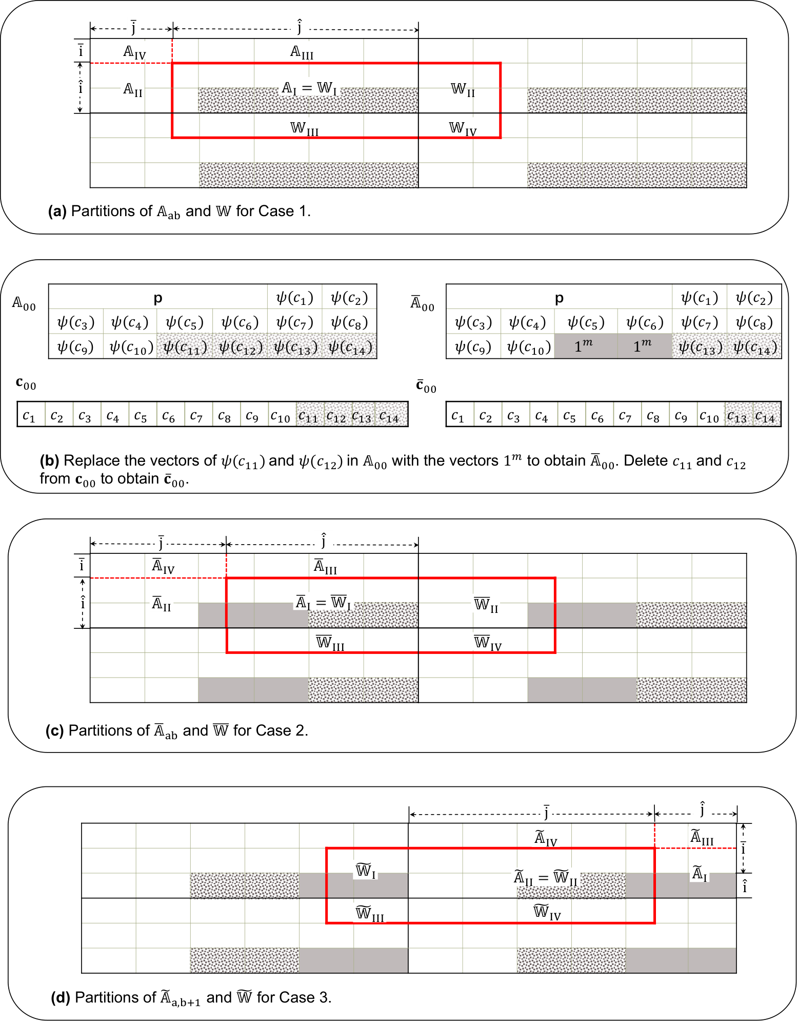
Suppose that $i=an+\bar{i}$ and $i^{\prime}=a^{\prime}n+\bar{i}$ for some $\bar{i}\in\llbracket n_{1}\rrbracket$ , and $j=bn+\bar{j}$ and $j^{\prime}=b^{\prime}n+\bar{j}$ for some $\bar{j}\in\llbracket n_{2}\rrbracket$ . Let $\hat{i}\in\llbracket n_{1}\rrbracket$ and $\hat{j}\in\llbracket n_{2}\rrbracket$ be the integers such that $\bar{i}+\hat{i}\equiv 0\pmod{n_{1}}$ and $\bar{j}+\hat{j}\equiv 0\pmod{n_{2}}$ . Shift $\mathbb{W}$ cyclically upwards $\hat{i}$ times and leftwards $\hat{j}$ times and denote the resulting array as $\mathbb{V}$ . Similarly, let $\mathbb{V}^{\prime}$ be the corresponding shifted array of $\mathbb{W}^{\prime}$ . Then $d_{H}(\mathbb{W},\mathbb{W}^{\prime})=d_{H}(\mathbb{V},\mathbb{V}^{\prime})$ . Since thickness is bounded by a constant, we have $\log n_{1}/\log n_{2}=O(1)$ , and then $(n_{R}-k_{R})m<n_{2}$ . It follows that the check bits of $\mathbb{A}_{\alpha\beta}$ appear in the last row $\mathbb{A}_{\alpha\beta}[n_{1}-1,n_{1}-1][n_{2}-(n_{R}-k_{R})m,n_{2}-1]$ . To estimate $d_{H}(\mathbb{V},\mathbb{V}^{\prime})$ , we proceed in three cases, depending on where the check bits of $\mathbb{V}$ and $\mathbb{V}^{\prime}$ come from.

Case 1: $\bar{j}\in[0,n_{2}-(n_{R}-k_{R})m-1]$ . As shown in Fig. 5(a), we partition $\mathbb{W}$ into four blocks by setting

	$\displaystyle\mathbb{W}_{\textup{I}}=\mathbb{W}[0,\hat{i}-1][0,\hat{j}-1],$	$\displaystyle\ \mathbb{W}_{\textup{II}}=\mathbb{W}[0,\hat{i}-1][\hat{j},n_{2}-1],$
	$\displaystyle\mathbb{W}_{\textup{III}}=\mathbb{W}[\hat{i},n_{1}-1][0,\hat{j}-1],$	$\displaystyle\ \mathbb{W}_{\textup{IV}}=\mathbb{W}[\hat{i},n_{1}-1][\hat{j},n_{2}-1],$

and partition $\mathbb{A}_{ab}$ into four blocks by setting

	$\displaystyle\mathbb{A}_{\textup{I}}=\mathbb{A}_{ab}[\bar{i},n_{1}-1][\bar{j},n_{2}-1],$	$\displaystyle\ \mathbb{A}_{\textup{II}}=\mathbb{A}_{ab}[\bar{i},n_{1}-1][0,\bar{j}-1],$
	$\displaystyle\mathbb{A}_{\textup{III}}=\mathbb{A}_{ab}[0,\bar{i}-1][\bar{j},n_{2}-1],$	$\displaystyle\ \mathbb{A}_{\textup{IV}}=\mathbb{A}_{ab}[0,\bar{i}-1][0,\bar{j}-1].$

Then we have

\mathbb{V}=\left(\begin{array}[]{cc}\mathbb{W}_{\textup{IV}}&\mathbb{W}_{\textup{III}}\\ \mathbb{W}_{\textup{II}}&\mathbb{W}_{\textup{I}}\end{array}\right),\mathbb{A}_{ab}=\left(\begin{array}[]{cc}\mathbb{A}_{\textup{IV}}&\mathbb{A}_{\textup{III}}\\ \mathbb{A}_{\textup{II}}&\mathbb{A}_{\textup{I}}\end{array}\right),

and $\mathbb{W}_{\textup{I}}=\mathbb{A}_{\textup{I}}.$

Notice that all these blocks, except $\mathbb{W}_{\textup{I}}$ and $\mathbb{A}_{\textup{I}}$ , do not contain check bits, and $(\boldsymbol{\sigma}_{0},\boldsymbol{\sigma}_{1}\ldots,\boldsymbol{\sigma}_{M-1})$ is a Gray code. It follows that

	$\displaystyle d_{B}(\mathbb{W}_{\textup{II}},\mathbb{A}_{\textup{II}})\leq d_{H}(\boldsymbol{\sigma}_{a}\boldsymbol{\sigma}_{b},\boldsymbol{\sigma}_{a}\boldsymbol{\sigma}_{b+1})\leq 1,$
	$\displaystyle d_{B}(\mathbb{W}_{\textup{III}},\mathbb{A}_{\textup{III}})\leq d_{H}(\boldsymbol{\sigma}_{a}\boldsymbol{\sigma}_{b},\boldsymbol{\sigma}_{a+1}\boldsymbol{\sigma}_{b})\leq 1,$
	$\displaystyle\textup{and \ }d_{B}(\mathbb{W}_{\textup{IV}},\mathbb{A}_{\textup{IV}})\leq d_{H}(\boldsymbol{\sigma}_{a}\boldsymbol{\sigma}_{b},\boldsymbol{\sigma}_{a+1}\boldsymbol{\sigma}_{b+1})\leq 2.$

So,

d_{B}(\mathbb{V},\mathbb{A}_{ab})\leq d_{B}(\mathbb{W}_{\textup{I}},\mathbb{A}_{\textup{I}})+d_{B}(\mathbb{W}_{\textup{II}},\mathbb{A}_{\textup{II}})+d_{B}(\mathbb{W}_{\textup{III}},\mathbb{A}_{\textup{III}})+d_{B}(\mathbb{W}_{\textup{IV}},\mathbb{A}_{\textup{IV}})\leq 4.

With the same argument, we can get $d_{B}(\mathbb{V}^{\prime},\mathbb{A}_{a^{\prime}b^{\prime}})\leq 4$ . Hence,

d_{H}(\mathbb{V},\mathbb{V}^{\prime})\geq d_{B}(\mathbb{V},\mathbb{V}^{\prime})\geq d_{B}(\mathbb{A}_{ab},\mathbb{A}_{a^{\prime}b^{\prime}})-8=d_{H}(\mathbfsl{c}_{ab},\mathbfsl{c}_{a^{\prime}b^{\prime}})-8\geq d.

Case 2: $\bar{j}\in[n_{2}-(n_{R}-k_{R})m,n_{2}-(n_{R}-k_{R})m/2-1]$ . For $\alpha,\beta\in\llbracket M\rrbracket$ , we change the bits in the block $\mathbb{A}_{\alpha\beta}[n_{1}-1,n_{1}-1][n_{2}-(n_{R}-k_{R})m,n_{2}-(n_{R}-k_{R})m/2-1]$ to one and denote the resulting array as $\bar{\mathbb{A}}_{\alpha\beta}$ . Let $\bar{\mathbfsl{c}}_{\alpha\beta}$ be the shortened codeword of $\mathbfsl{c}_{\alpha,\beta}$ by deleting the subword $\mathbfsl{c}_{\alpha\beta}[k_{R},n_{R}-(n_{R}-k_{R})/2-1]$ (see Fig. 5(b)). Then we have

d_{B}(\bar{\mathbb{A}}_{\alpha\beta},\bar{\mathbb{A}}_{\alpha^{\prime}\beta^{\prime}})=d_{H}(\bar{\mathbfsl{c}}_{\alpha\beta},\bar{\mathbfsl{c}}_{\alpha^{\prime}\beta^{\prime}})\geq(n_{R}-(n_{R}-k_{R})/2)-k_{R}+1\geq d+8.

(2)

Now, let $\bar{\mathbb{W}}$ , $\bar{\mathbb{W}}^{\prime}$ , $\bar{\mathbb{V}}$ and $\bar{\mathbb{V}}^{\prime}$ be the corresponding arrays of ${\mathbb{W}}$ , ${\mathbb{W}}^{\prime}$ , ${\mathbb{V}}$ and ${\mathbb{V}}^{\prime}$ with some check bits being changed to one. As in Case 1, we can show that

d_{B}(\bar{\mathbb{V}},\bar{\mathbb{A}}_{ab})\leq 4\textup{\ and\ }d_{B}(\bar{\mathbb{V}}^{\prime},\bar{\mathbb{A}}_{ab}^{\prime})\leq 4.

(3)

The only difference is that $\bar{\mathbb{W}}_{\textup{II}}$ , $\bar{\mathbb{A}}_{\textup{II}}$ , $\bar{\mathbb{W}}^{\prime}_{\textup{II}}$ , and $\bar{\mathbb{A}}^{\prime}_{\textup{II}}$ may contain the check bits. However, these bits are set to one, so we have $d_{B}(\bar{\mathbb{W}}_{\textup{II}},\bar{\mathbb{A}}_{\textup{II}})\leq d_{H}(\boldsymbol{\sigma}_{a}\boldsymbol{\sigma}_{b},\boldsymbol{\sigma}_{a}\boldsymbol{\sigma}_{b+1})\leq 1$ , see Fig. 5(c).

It follows from (2) and (3) that

d_{B}(\bar{\mathbb{V}},\bar{\mathbb{V}}^{\prime})\geq d_{B}(\bar{\mathbb{A}}_{ab},\bar{\mathbb{A}}_{a^{\prime}b^{\prime}})-8\geq d,

and then

d_{H}(\mathbb{V},\mathbb{V}^{\prime})\geq d_{H}(\bar{\mathbb{V}},\bar{\mathbb{V}}^{\prime})\geq d_{B}(\bar{\mathbb{V}},\bar{\mathbb{V}}^{\prime})\geq d.

Case 3: $\bar{j}\in[n_{2}-(n_{R}-k_{R})m/2,n_{2}-1]$ . For $\alpha,\beta\in\llbracket M\rrbracket$ , we change the bits in the block $\mathbb{A}_{\alpha\beta}[n_{1}-1,n_{1}-1][n_{2}-(n_{R}-k_{R})m/2,n_{2}-1]$ to one and denote the resulting array as $\tilde{\mathbb{A}}_{\alpha\beta}$ . Let $\tilde{\mathbfsl{c}}_{\alpha\beta}$ be the shortened codeword of $\mathbfsl{c}_{\alpha,\beta}$ by deleting the last $(n_{R}-k_{R})/2$ bits.

Now, let $\tilde{\mathbb{W}}$ , $\tilde{\mathbb{W}}^{\prime}$ , $\tilde{\mathbb{V}}$ and $\tilde{\mathbb{V}}^{\prime}$ be the corresponding arrays of ${\mathbb{W}}$ , ${\mathbb{W}}^{\prime}$ , ${\mathbb{V}}$ and ${\mathbb{V}}^{\prime}$ . Again we use the strategy in Case 1 to show that

d_{H}(\mathbb{V},\mathbb{V}^{\prime})\geq d_{H}(\tilde{\mathbb{V}},\tilde{\mathbb{V}}^{\prime})\geq d_{B}(\tilde{\mathbb{V}},\tilde{\mathbb{V}}^{\prime})\geq d_{B}(\tilde{\mathbb{A}}_{a,b+1},\tilde{\mathbb{A}}_{a^{\prime},b^{\prime}+1})-8\geq d.

We note that in this case we need to partition $\tilde{\mathbb{A}}_{a,b+1}$ instead of $\tilde{\mathbb{A}}_{ab}$ , see Fig. 5(d).

Refer to caption — Figure 5: An example with $n_{1}=3$ and $n_{2}=6m$ to illustrate the proof of Lemma 17. The black lines enclose the arrays $\mathbb{A}_{ab}$ , $\mathbb{A}_{a,b+1}$ , $\mathbb{A}_{a+1,b}$ and $\mathbb{A}_{a+1,b+1}$ . The red lines enclose the subarray $\mathbb{W}$ . The empty blocks represent the vectors of message bits. The blocks with dots represent the vectors of check bits. The solid blocks represent the vectors $1^{m}$ .

Theorem 18.

The array $\mathbb{A}$ in Construction 2 is an $(n_{1}\times n_{2},d)$ -RPA.

Proof.

Let $\mathbb{W}$ and $\mathbb{W}^{\prime}$ be two distinct subarrays of dimension $n_{1}\times n_{2}$ in $\mathbb{A}$ . Assume that $\mathbb{W}=\mathbb{A}[i,i+n_{1}-1][j,j+n_{2}-1]$ and $\mathbb{W}^{\prime}=\mathbb{A}[i^{\prime},i^{\prime}+n_{1}-1][j^{\prime},j^{\prime}+n_{2}-1]$ , where $(i,j)\not=(i^{\prime},j^{\prime})$ . From Lemma 17, we have $d_{H}(\mathbb{W},\mathbb{W}^{\prime})\geq d$ when $i\equiv i^{\prime}\pmod{n_{1}}$ and $j\equiv j^{\prime}\pmod{n_{2}}$ . Now we consider the case where $i\not\equiv i^{\prime}\pmod{n_{1}}$ or $j\not\equiv j^{\prime}\pmod{n_{2}}$ . Let $\hat{i}\in[n_{1}]$ and $\hat{j}\in[n_{2}]$ such that $i+\hat{i}\equiv 0~({\rm mod~}n_{1})$ and $j+\hat{j}\equiv 0~({\rm mod~}n_{2})$ . So we have $i^{\prime}+\hat{i}\not\equiv 0~({\rm mod~}n_{1})$ or $j^{\prime}+\hat{j}\not\equiv 0~({\rm mod~}n_{2})$ . It follows from Lemma 16 that $\mathbb{W}[\hat{i},\hat{i}][\hat{j},\hat{j}+4m-1]=\mathbfsl{p}$ and $d_{H}(\mathbb{W}^{\prime}[\hat{i},\hat{i}][\hat{j},\hat{j}+4m-1],\mathbfsl{p})\geq d$ . Hence

d_{H}(\mathbb{W},\mathbb{W}^{\prime})\geq d_{H}(\mathbb{W}[\hat{i},\hat{i}][\hat{j},\hat{j}+4m-1],\mathbb{W}^{\prime}[\hat{i},\hat{i}][\hat{j},\hat{j}+4m-1])\geq d,

which completes the proof.

Corollary 19.

Let $\mathbb{W}$ be a window of area $A$ and thickness bounded by a constant. Then there is a binary RPA for $\mathbb{W}$ with distance $d$ and redundancy at most

4.21d\log{A}+35.79\log{A}+o(1),

provided $A$ is large enough.

Proof.

The RPA $\mathbb{A}$ in Construction 2 has dimension $(n_{1}M)\times(n_{2}M)$ , where $M=q^{k_{R}/2}$ . So, its redundancy is given by

n_{1}n_{2}-\log(n_{1}n_{2}M^{2})=A-k_{R}\log q-\log A,

where $k_{R}=n_{R}-2(d+7)=A/m-2d-18,$ and

\log q\geq\log(r-r^{\theta})=\log r+\log\left(1-\frac{1}{r^{1-\theta}}\right)\geq\log r-\frac{\log e}{r^{1-\theta}-1}.

(4)

Recall that $\theta=0.525$ , and so, $m={\log A}/(1-\theta)\geq({3}/{2})\log A.$ It follows that

	$\displaystyle r$	$\displaystyle=\sum_{i=d}^{m}{m\choose i}=2^{m}\left[1-\sum_{i=0}^{d-1}{m\choose i}\frac{1}{2^{m}}\right]\geq 2^{m}\left[1-\exp\left(-\frac{2(m/2-d+1)^{2}}{m}\right)\right]$
		$\displaystyle\geq 2^{m}\left(1-e^{-\frac{2m}{3\log e}}\right)\geq 2^{m}\left(1-\frac{1}{A}\right).$

Then we have

\displaystyle\log r\geq m+\log\left(1-\frac{1}{A}\right)\geq m-\frac{\log e}{A-1}.

(5)

On the other hand,

\displaystyle r^{1-\theta}\geq\left(\frac{2^{m}}{2}\right)^{1-\theta}=\frac{A}{2^{1-\theta}}.

(6)

Combining (4), (5) and (6), we get

\displaystyle\log q\geq m-O\left(\frac{1}{A}\right).

Hence, the redundancy of $\mathbb{A}$ is at most

	$\displaystyle A\ -\$	$\displaystyle\left(\frac{A}{m}-2d-18\right)\left(m-O\left(\frac{1}{A}\right)\right)-\log A$
	$\displaystyle=$	$\displaystyle\ \frac{2d}{1-\theta}\log A+\frac{18}{1-\theta}\log A-\log A+o(1)$
	$\displaystyle\approx$	$\displaystyle\ 4.21d\log A+{36.89}\log A+o(1).$

To conclude, we provide an efficient locating algorithm for the array $\mathbb{A}$ in Construction 2. Let $\chi$ be a map from $\mathbb{F}_{2}^{m}$ to $\mathbb{F}_{q}$ such that $\chi(\psi(x))=x$ for all $x\in\mathbb{F}_{q}$ and $\chi(\mathbfsl{v})=0$ for all $\mathbfsl{v}\not\in\{\psi(x):x\in\mathbb{F}_{q}\}$ .

We briefly describe Algorithm 2. Suppose that $\mathbb{W}$ is an $n_{1}\times n_{2}$ subarray of $\mathbb{A}$ that is corrupted at $e$ positions with $e\leq(d-1)/2$ . So there is a unique pair $(i,j)$ such that $d_{H}(\mathbb{A}[i,i+n-1][j,j+n-1],\mathbb{W})\leq(d-1)/2$ . Assume that $i=an_{1}+\bar{i}$ and $j=bn_{2}+\bar{j}$ with $\bar{i}\equiv i\pmod{n_{1}}$ and $\bar{j}\equiv j\pmod{n_{2}}$ . In what follows, we briefly describe how to determine $a,b,\bar{i}$ and $\bar{j}$ .

(I)

We first use Lemma 16 to determine $\bar{i}$ and $\bar{j}$ .
(II)

Next, we rotate $\mathbb{W}$ appropriately to obtain $\mathbb{V}$ , so that the concatenation of the rows of $\mathbb{V}$ , denoted as $\mathbfsl{v}$ , is the binary image obtained from either a $q$ -ary codeword $\mathbfsl{c}_{a,b}$ or a concatenation of some shortened codewords $\mathbfsl{c}_{a,b}$ , $\mathbfsl{c}_{a+1,b}$ , $\mathbfsl{c}_{a,b+1}$ , and $\mathbfsl{c}_{a+1,b+1}$ . Since $\mathbfsl{v}$ is obtained via the map $\psi$ and prepending the string $\mathbfsl{p}$ , we reverse this process to obtain the $q$ -ary estimate $\mathbfsl{u}$ .
(III)

Finally, depending on the value of $\bar{j}$ , we apply the Reed-Solomon decoding algorithm ${\rm dec}_{\rm RS}$ to find either $\mathbfsl{c}_{a,b}$ (when $\bar{j}\in[0,n_{2}-2(d+7)m-1]$ ), some shortened version of $\mathbfsl{c}_{a,b}$ (when $\bar{j}\in[n_{2}-2(d+7)m,n_{2}-(d+7)m-1]$ ), or some shortened version of $\mathbfsl{c}_{a,b+1}$ (when $j\in[n_{2}-(d+7)m,n_{2}-1]$ ). Therefore, we determine $a$ and $b$ and hence, obtain $i=an_{1}+\hat{i}$ and $j=bn_{2}+\hat{j}$ .

The first step above requires $\ell_{p}n_{1}n_{2}$ comparisons. The Reed-Solomon decoding runs in $O(n_{R}^{3})=O((n_{1}n_{2})^{3})$ time, and the decoding of Gray codes runs in $O(k_{R}(\log q)^{2})=O(n_{1}n_{2}(\log(n_{1}n_{2}))^{2})$ time. Therefore, Algorithm 1 can determine the location in $O((n_{1}n_{2})^{3})$ , or equivalently $O(A^{3})$ time.

Input: an

n_{1}\times n_{2}

window

\mathbb{W}

of area

A

and thickness bounded by a constant

Output: a position

(i,j)\triangleq(an_{1}+\bar{i},bn_{2}+\bar{j})

such that

d_{H}(\mathbb{A}[i,i+n_{1}-1][j,j+n_{2}-1],\mathbb{W})\leq(d-1)/2

m\leftarrow\frac{\log A}{1-\theta}

n_{R}\leftarrow n_{1}(n_{2}/m)-4

k_{R}\leftarrow n_{R}-2(d+7)

(\hat{i},\hat{j})\leftarrow

unique tuple such that

d_{H}(\mathbb{W}[\hat{i},\hat{i}][\hat{j},\hat{j}+4m-1],\mathbfsl{p})\leq(d-1)/2

Set

\bar{i}\in\llbracket n_{1}\rrbracket

such that

\bar{i}+\hat{i}\equiv 0~({\rm mod~}n_{1})

Set

\bar{j}\in\llbracket n_{2}\rrbracket

such that

\bar{j}+\hat{j}\equiv 0~({\rm mod~}n_{2})

\mathbb{V}\leftarrow

the array obtained by shifting

\mathbb{W}

cyclically upwards

\hat{i}

times and leftwards

\hat{j}

times

\mathbfsl{v}\leftarrow

the concatenation of the rows of

\mathbb{V}

\mathbfsl{u}\leftarrow\chi(\mathbfsl{v}[4m,5m-1])\chi(\mathbfsl{v}[5m,6m-1])\chi(\mathbfsl{v}[6m,7m-1])\cdots\chi(\mathbfsl{v}[n_{1}n_{2}-m,n_{1}n_{2}-1])

\bar{j}\in[0,n_{2}-2(d+7)m-1]

then

\mathbfsl{c}\leftarrow{\rm dec}_{\rm RS}^{(n_{R},k_{R})}(\mathbfsl{u})

else if

\bar{j}\in[n_{2}-2(d+7)m,n_{2}-(d+7)m-1]

then

\mathbfsl{u}^{s}\leftarrow

the shortened codeword

\mathbfsl{u}[0,k_{R}-1]\mathbfsl{u}[k_{R}+(d+7),n_{R}-1]

\mathbfsl{c}\leftarrow{\rm dec}_{\rm RS}^{(n_{R}-(d+7),k_{R})}(\mathbfsl{u}^{s})

else

\mathbfsl{u}^{s}\leftarrow

the shortened codeword

\bar{\mathbfsl}{c}[0,k_{R}+d+6]

\mathbfsl{c}\leftarrow{\rm dec}_{\rm RS}^{(n_{R}-(d+7),k_{R})}(\mathbfsl{u}^{s})

a\leftarrow{\rm dec}_{\rm Gray}(\mathbfsl{c}[0,k_{R}/2-1])

\bar{j}\in[0,n_{2}-(d+7)m-1]

then

b\leftarrow{\rm dec}_{\rm Gray}(\mathbfsl{c}[k_{R}/2,k_{R}-1])

else

b+1\leftarrow{\rm dec}_{\rm Gray}(\mathbfsl{c}[k_{R}/2,k_{R}-1])

return

(an_{1}+\bar{i},bn_{2}+\bar{j})

Algorithm 2 Locating algorithm for the array

\mathbb{A}

in Construction 2

5 Binary Positioning Arrays with Constant Rank Distance

We continue our investigation of binary robust positioning arrays. In this section, we consider the scenario where the error patterns are confined to a certain number of rows or columns (or both). To correct for such errors, Roth demonstrated that it suffices to consider codes in the rank distance metric [16].

For two matrices $\mathbb{M}_{1}$ and $\mathbb{M}_{2}$ of the same dimension, the rank distance between them, denoted as $d_{R}(\mathbb{M}_{1},\mathbb{M}_{2})$ , is defined as the rank of their difference, i.e., $d_{R}(\mathbb{M}_{1},\mathbb{M}_{2})\triangleq{\rm rank}(\mathbb{M}_{1}-\mathbb{M}_{2})$ . In this section, we modify Construction 2 to produce a binary positioning array of strength $n_{1}\times n_{2}$ and rank distance $d$ , i.e., a large array in which the rank distance between any two $n_{1}\times n_{2}$ submatrices is at least $d$ . Since a code ${\mathcal{M}}\subseteq\mathbb{F}_{q}^{n_{1}\times n_{2}}$ with minimum rank distance $d$ satisfies the Singleton bound, i.e., $|{\mathcal{M}}|\leq q^{n_{2}(n_{1}-d+1)}$ , the redundancy of such an array should be at least $n_{2}(d-1)-O(1)$ .

To present our construction, we require the concept of maximum rank distance (MRD) codes.

Theorem 20 (Maximum rank distance (MRD) code [6]).

Let $q$ be a prime power. Suppose that $N_{1}\leq N_{2}$ . Then there exists a linear code ${\mathcal{M}}\leq F_{q}^{N_{1}\times N_{2}}$ of rank distance $d$ and dimension $N_{2}(N_{1}-d+1)$ .

We also need to choose a new marker $\mathbb{P}$ . Fix $d$ and let $m$ be an integer such that $m(m-d+1)=\log(n_{1}n_{2})$ . Let $\mathbb{P}$ be a $4m\times 4m$ array in which

(i)

the diagonal is $0^{4m-\ell}\mathbfsl{u}$ , where $\mathbfsl{u}$ is the $d$ -auto-cyclic vector provided in (1);
(ii)

the $d\times d$ subarrays at the right top corner and left bottom corner are identity matrices;
(iii)

the symbols in all the other entries are $0$ .

Let ${\mathcal{M}}\subseteq\mathbb{F}_{2}^{m\times m}$ be an MRD code of rank distance $d$ and dimension $m(m-d+1)$ . Suppose that both $n_{1}$ and $n_{2}$ are divisible by $m$ . Set $n_{R}\triangleq\frac{n_{1}n_{1}}{m^{2}}-16$ and $k_{R}\triangleq n_{R}-24$ . Choose a prime power $q$ such that $n_{R}\leq q<2^{m(m-d+1)}$ and set $M\triangleq q^{k_{R}/2}$ . Take an arbitrary injective map $\psi$ from $\mathbb{F}_{q}$ to ${\mathcal{M}}\backslash\{\mathbf{0}\}$ , where $\mathbf{0}$ is the all-zero matrix. So $\psi$ maps the elements of $\mathbb{F}_{q}$ to $m\times m$ matrices of rank at least $d$ .

Construction 3. Let ${\mathcal{G}}=(\boldsymbol{\sigma}_{0},\boldsymbol{\sigma}_{1},\ldots,\boldsymbol{\sigma}_{M-1})$ be a $(k_{R}/2,q)$ -Gray code and consider a Reed-Solomon code of length $n_{R}$ and dimension $k_{R}$ over $\mathbb{F}_{q}$ . For each $0\leq i,j\leq M-1$ , set $\mathbfsl{c}_{ij}={\rm enc}_{\rm RS}^{(n_{R},k_{R})}(\boldsymbol{\sigma}_{i}\boldsymbol{\sigma}_{j})$ .

For each $\mathbfsl{c}_{ij}$ , apply the map $\psi$ to the symbols of $\mathbfsl{c}_{ij}$ to obtain $n_{R}$ $m\times m$ matrices of rank at least $d$ . Since $n_{R}=(n_{1}n_{2})/m^{2}-16$ and $n_{R}-k_{R}=24$ , tile these $n_{R}$ matrices together with the marker $\mathbb{P}$ to form an $n_{1}\times n_{2}$ array $\mathbb{A}_{ij}$ (see Fig. 6) such that

(i)

$\mathbb{A}_{ij}[0,4m-1][0,4m-1]=\mathbb{P}$ ;
(ii)

for each $\ell\in\{1,2,3\}$ , $\mathbb{A}_{ij}[n_{1}-2m\ell,n_{1}-2m(\ell-1)-1][n_{2}-4m\ell,n_{2}-4m(\ell-1)-1]$ comprises eight $m\times m$ submatrices, each of which corresponds to a check bit of $\mathbfsl{c}_{ij}$ .

Finally, construct a large array $\mathbb{A}$ as

\mathbb{A}=\left(\begin{array}[]{cccc}\mathbb{A}_{00}&\mathbb{A}_{01}&\cdots&\mathbb{A}_{0,M-1}\\ \mathbb{A}_{10}&\mathbb{A}_{11}&\cdots&\mathbb{A}_{1,M-1}\\ \vdots&\vdots&\ddots&\vdots\\ \mathbb{A}_{M-1,0}&\mathbb{A}_{M-1,1}&\cdots&\mathbb{A}_{M-1,M-1}\end{array}\right).

Figure 6: An example for the matrix

A_{ij}

in Construction 3 with

n_{1}=11m

and

n_{2}=17m

. The blue cells represent the message bits and the yellow cells represent the check bits.

Lemma 21.

(i)

If $i+i_{0}\equiv 0~({\rm mod~}n_{1})$ and $j+j_{0}\pmod{n_{2}}$ , then $\mathbb{W}[i,i+4m-1][j,j+4m-1]=\mathbb{P}$ .
(ii)

If $i+i_{0}\not\equiv 0~({\rm mod~}n_{1})$ or $j+j_{0}\not\equiv 0~({\rm mod~}n_{2})$ , then $d_{R}(\mathbb{W}[i,i+4m-1][j,j+4m-1],\mathbb{P})\geq d$ .

Proof.

For simplicity, we assume that $n_{1}=n_{2}=n$ . The case of $n_{1}\not=n_{2}$ can be proceeded similarly. Let $\hat{i},\hat{j}\in\llbracket n\rrbracket$ such that $\hat{i}+i_{0}\equiv 0~({\rm mod~}n)$ and $\hat{j}+j_{0}\equiv 0~({\rm mod~}n)$ . We consider the array $\mathbb{V}$ , which is obtained by shifting $\mathbb{W}$ cyclically upwards $\hat{i}$ times and leftwards $\hat{j}$ times. Then $\mathbb{V}[0,4m-1][0,4m-1]=\mathbb{P}$ and it suffices to show that $d_{R}(\mathbb{V}[i,i+4m-1][j,j+4m-1],\mathbb{P})\geq d$ for $(i,j)\in\llbracket n\rrbracket^{2}\backslash\{(0,0)\}$ . Write ${\rm Diag}(\mathbfsl{x})$ for a diagonal matrix whose diagonal is $\mathbfsl{x}$ .

We first assume $i=j$ . Similar to the proof of Lemma 7, we consider the following cases.

Case 1a: $i\in[1,d]$ . Then $\mathbb{P}[4m-\ell-i,4m-1-i][4m-\ell-i,4m-1-i]={\rm Diag}(0^{i}\mathbfsl{u}[0,{\ell-i}-1])$ . On the other hand, the corresponding subarray in $\mathbb{V}[i,i+4m-1][j,j+4m-1]$ is $\mathbb{V}[4m-\ell,4m-1][4m-\ell,4m-1]$ , which is equal to ${\rm Diag}(\mathbfsl{u})$ . Due to the property of $\mathbfsl{u}$ , the rank distance between them is at least $d$ and so $d_{R}(\mathbb{V}[i,i+4m-1][j,j+4m-1],\mathbb{P})\geq d$ .

Case 1b: $i\in[d+1,4m-d]$ . Since $4m-\ell>\ell$ , $\mathbb{V}[i,i+4m-\ell-1][i,i+4m-\ell-1]$ contains at least one subarray which is equal to ${\rm Diag}(1^{d})$ . Note that $\mathbb{P}[0,4m-\ell-1][0,4m-\ell-1]=\mathbf{0}$ . The rank distance between $\mathbb{V}[i,i+4m-\ell-1][i,i+4m-\ell-1]$ and $\mathbb{P}[0,4m-\ell-1][0,4m-\ell-1]$ is at least $d$ and so we have $d_{R}(\mathbb{V}[i,i+4m-1][j,j+4m-1],\mathbb{P})\geq d$ .

Case 1c: $i\in[4m-d+1,n-(4m-\ell)]$ . Since $4m-\ell-d>3m$ , $\mathbb{V}[i+d,i+4m-\ell-1][i+d,i+4m-\ell-1]$ should contain at least one $m\times m$ subarray of rank at least $d$ . Noting that $\mathbb{P}[i+d,i+4m-\ell-1][i+d,i+4m-\ell-1]=\mathbf{0}$ , again we have $d_{R}(\mathbb{V}[i,i+4m-1][j,j+4m-1],\mathbb{P})\geq d$ .

Case 1d: $i\in[n-(4m-\ell)+1,n-d]$ . Since $i+4m-\ell-n\geq 1$ and $i+4m-\ell+d-1-n\leq 4m-\ell-1$ , we have $\mathbb{V}[i+4m-\ell,i+4m-\ell+d-1][i+4m-\ell,i+4m-\ell+d-1]=\mathbf{0}$ . Note that $\mathbb{P}[4m-\ell,4m-\ell+d-1]={\rm Diag}(1^{d})$ . It follows that $d_{R}(\mathbb{V}[i,i+4m-1][j,j+4m-1],\mathbb{P})\geq d$ .

Case 1e: $i\in[n-d+1,n-1]$ . Let $\delta=n-i$ , then $\delta\in[1,d-1]$ . We have

		$\displaystyle\mathbb{V}[i+4m-\ell,i+4m-1][i+4m-\ell,i+4m-1]$
	$\displaystyle=$	$\displaystyle\mathbb{V}[4m-\ell-\delta,4m-1-\delta][4m-\ell-\delta,4m-1-\delta]$
	$\displaystyle=$	$\displaystyle{\rm Diag}(0^{\delta}\mathbfsl{u}[0,\ell-\delta-1]).$

Since $\mathbb{P}[4m-\ell,4m-1][4m-\ell,4m-1]={\rm Diag}(\mathbfsl{u})$ , the rank distance between them is at least $d$ and so we have $d_{R}(\mathbb{V}[i,i+4m-1][j,j+4m-1],\mathbb{P})\geq d$ .

In the following we assume that $i<j$ ; the case of $i>j$ can be proceeded in the same way.

Case 2a: $j\in[1,4m-2d]$ . Then $d\leq 4m-d-j<4m-d-i$ and $4m-1-j<4m-1-i\leq 4m-1$ . It follows that the subarray $\mathbb{P}[4m-d-i,4m-1-i][4m-d-i,4m-1-i]$ is an upper triangular matrix with all entries on the diagonal being $0$ . On the other hand, in $\mathbb{V}[i,i+4m-1][j,j+4m-1]$ the corresponding subarray $\mathbb{V}[4m-d,4m-1][4m-d,4m-1]$ is an identity matrix. Hence the rank distance between $\mathbb{V}[i,i+4m-1][j,j+4m-1]$ and $\mathbb{P}$ is at least $d$ .

Case 2b: $j\in[4m-2d+1,n-(4m-\ell)]$ . In this case we estimate the rank distance between the submatrices

\mathbb{V}[i+2d,i+4m-\ell-1][j+2d,j+4m-\ell-1]

and $\mathbb{P}[2d,4m-\ell-1][2d,4m-\ell-1]$ . Since $4m\leq j+2d$ , $j+4m-\ell-1\leq n-1$ and $4m-\ell-2d>3m$ , the subarray $\mathbb{V}[i+2d,i+4m-\ell-1][j+2d,j+4m-\ell-1]$ always contains an $m\times m$ submatrix of rank at least $d$ . On the other hand, $\mathbb{P}[2d,4m-\ell-1][2d,4m-\ell-1]=\mathbf{0}$ . It follows that the rank distance between them is at least $d$ and so $d_{R}(\mathbb{V}[i,i+4m-1][j,j+4m-1],\mathbb{P})\geq d$ .

Case 2c: $j\in[n-(4m-\ell)+1,n-1]$ and $i\in[0,4m-\ell-d]$ . Then

\mathbb{V}[i,i+d-1][j+4m-d,j+4m-1]=\mathbb{V}[i,i+d-1][j+4m-d-n,j+4m-1-n].

Since $0\leq i<i+d-1\leq 4m-\ell-1$ and $\ell-d<j+4m-d-n<j+4m-1-n<4m-1$ , the subarray $\mathbb{V}[i,i+d-1][j+4m-d,j+4m-1]$ is an upper triangular matrix with all entries on the diagonal being $0$ . Note that in $\mathbb{P}$ the corresponding subarray $\mathbb{P}[0,d-1][4m-d,4m-1]=\mathbb{I}_{d}$ . Thus the rank distance between $\mathbb{V}[i,i+4m-1][j,j+4m-1]$ and $\mathbb{P}$ is at least $d$ .

Case 2d: $j\in[n-(4m-\ell)+1,n-1]$ and $i\in[4m-\ell-d+1,n-(4m-\ell)]$ . Then $4m<i+\ell+d<i+4m-\ell-1\leq n-1$ . Since $4m-2\ell-d>3m$ , the subarray $\mathbb{W}[i+\ell+d,i+4m-\ell-1][j+\ell+d,j+4m-\ell-1]$ always contains an $m\times m$ submatrix of rank at least $d$ . Note that the corresponding subarray $\mathbb{P}[\ell+d,4m-\ell-1][\ell+d,4m-\ell-1]=\mathbf{0}$ . It follows that $d_{R}(\mathbb{V}[i,i+4m-1][j,j+4m-1],\mathbb{P})\geq d$ .

Case 2e: $j\in[n-(4m-\ell)+1,n-1]$ and $i\in[n-(4m-\ell)+1,n-1]$ . Then

	$\displaystyle\mathbb{V}$	$\displaystyle[i+4m-d,i+4m-1][j+4m-d,j+4m-1]$
		$\displaystyle=\mathbb{V}[i+4m-d-n,i+4m-1-n][j+4m-d-n,j+4m-1-n].$

Since $\ell-d<i+4m-d-n<j+4m-d-n$ and $i+4m-1-n<j+4m-1-n<4m-1$ , the subarray $\mathbb{V}[i,i+d-1][j+4m-d,j+4m-1]$ is a lower triangular matrix with all entries on the diagonal being $0$ . Note that in $\mathbb{P}$ the corresponding subarray $\mathbb{P}[4m-d,4m-1][4m-d,4m-1]=\mathbb{I}_{d}$ . Thus the rank distance between $\mathbb{V}[i,i+4m-1][j,j+4m-1]$ and $\mathbb{P}$ is at least $d$ .

Lemma 22.

Proof.

Suppose that $i=an_{1}+\bar{i}$ and $i^{\prime}=a^{\prime}n_{1}+\bar{i}$ for some $\bar{i}\in\llbracket n_{1}\rrbracket$ , and $j=bn_{2}+\bar{j}$ and $j^{\prime}=b^{\prime}n_{2}+\bar{j}$ for some $\bar{j}\in\llbracket n_{2}\rrbracket$ . Let $\hat{i}\in\llbracket n_{1}\rrbracket$ and $\hat{j}\in\llbracket n_{2}\rrbracket$ be the integers such that $\bar{i}+\hat{i}\equiv 0\pmod{n_{1}}$ and $\bar{j}+\hat{j}\equiv 0\pmod{n_{2}}$ . Shift $\mathbb{W}$ cyclically upwards $\hat{i}$ times and leftwards $\hat{j}$ times and denote the resulting array as $\mathbb{V}$ . Similarly, let $\mathbb{V}^{\prime}$ be the corresponding shifted array of $\mathbb{W}^{\prime}$ . Then $d_{R}(\mathbb{W},\mathbb{W}^{\prime})=d_{R}(\mathbb{V},\mathbb{V}^{\prime})$ . To estimate $d_{R}(\mathbb{V},\mathbb{V}^{\prime})$ , we proceed in three cases, depending on where the check bits of $\mathbb{V}$ and $\mathbb{V}^{\prime}$ come from. Similar to the proof of Lemma 17, for any two subarrays $\mathbb{M}$ and $\mathbb{M}^{\prime}$ in $\mathbb{A}$ which are of same dimension and in the same modular position, we use $d_{S}(\mathbb{M},\mathbb{M}^{\prime})$ to denote the number of different (truncated) $m\times m$ subarrays in $\mathbb{M}$ and $\mathbb{M}^{\prime}$ .

Case 1: $\bar{i}\in[0,n_{1}-2m-1]$ and $\bar{j}\in[0,n_{2}-4m-1]$ . For $\alpha,\beta\in\llbracket M\rrbracket$ , we change the bits in the subarrays $\mathbb{A}_{\alpha\beta}[n_{1}-6m,n_{1}-4m-1][n_{2}-12m,n_{2}-8m-1]$ and $\mathbb{A}_{\alpha\beta}[n_{1}-4m,n_{1}-2m-1][n_{2}-8m,n_{2}-4m-1]$ to one and denote the resulting array as $\bar{\mathbb{A}}_{\alpha\beta}$ . Let $\bar{\mathbfsl{c}}_{\alpha\beta}$ be the corresponding shortened codeword of length $n_{R}-16$ . Then we have

\displaystyle d_{S}(\bar{\mathbb{A}}_{\alpha\beta},\bar{\mathbb{A}}_{\alpha^{\prime}\beta^{\prime}})=d_{H}(\bar{\mathbfsl{c}}_{\alpha\beta},\bar{\mathbfsl{c}}_{\alpha^{\prime}\beta^{\prime}})\geq(n_{R}-16)-k_{R}+1\geq 9.

(7)

\bar{\mathbb{V}}=\left(\begin{array}[]{cc}\bar{\mathbb{W}}_{\textup{IV}}&\bar{\mathbb{W}}_{\textup{III}}\\ \bar{\mathbb{W}}_{\textup{II}}&\bar{\mathbb{W}}_{\textup{I}}\end{array}\right),\bar{\mathbb{A}}_{ab}=\left(\begin{array}[]{cc}\bar{\mathbb{A}}_{\textup{IV}}&\bar{\mathbb{A}}_{\textup{III}}\\ \bar{\mathbb{A}}_{\textup{II}}&\bar{\mathbb{A}}_{\textup{I}}\end{array}\right),\textup{\ and \ }\bar{\mathbb{W}}_{\textup{I}}=\bar{\mathbb{A}}_{\textup{I}}.

Furthermore, we have

d_{S}(\bar{\mathbb{W}}_{\textup{II}},\bar{\mathbb{A}}_{\textup{II}})\leq 1,\ d_{S}(\bar{\mathbb{W}}_{\textup{III}},\bar{\mathbb{A}}_{\textup{III}})\leq 1,\textup{\ and \ }d_{S}(\bar{\mathbb{W}}_{\textup{IV}},\bar{\mathbb{A}}_{\textup{IV}})\leq 2.

It follows that $d_{S}(\bar{\mathbb{V}},\bar{\mathbb{A}}_{ab})\leq 4.$ With the same argument, we can get $d_{B}(\bar{\mathbb{V}}^{\prime},\bar{\mathbb{A}}_{a^{\prime}b^{\prime}})\leq 4$ . Hence,

d_{S}(\mathbb{V},\mathbb{V}^{\prime})\geq d_{S}(\bar{\mathbb{V}},\bar{\mathbb{V}}^{\prime})\geq d_{S}(\bar{\mathbb{A}}_{ab},\bar{\mathbb{A}}_{a^{\prime}b^{\prime}})-8\geq 1.

So we can find a pair of distinct $m\times m$ subarrays in the same position of $\mathbb{V}$ and $\mathbb{V}^{\prime}$ . Since these two subarrays are codewords of an MRD code, the rank distance between them is at least $d$ . Thus $d_{R}(\mathbb{W},\mathbb{W}^{\prime})=d_{R}(\mathbb{V},\mathbb{V}^{\prime})\geq d$ .

Case 2: $\bar{i}\in[0,n_{1}-4m-1]$ and $\bar{j}\in[n_{2}-4m,n_{2}-1]$ . We change the bits in the subarrays $\mathbb{A}_{\alpha\beta}[n_{1}-6m,n_{1}-4m-1][n_{2}-12m,n_{2}-8m-1]$ and $\mathbb{A}_{\alpha\beta}[n_{1}-2m,n_{1}-1][n_{2}-4m,n_{2}-1]$ to one and denote the resulting array as $\tilde{\mathbb{A}}_{\alpha\beta}$ . Let $\tilde{\mathbb{W}}$ , $\tilde{\mathbb{W}}^{\prime}$ , $\tilde{\mathbb{V}}$ and $\tilde{\mathbb{V}}^{\prime}$ be the corresponding arrays of ${\mathbb{W}}$ , ${\mathbb{W}}^{\prime}$ , ${\mathbb{V}}$ and ${\mathbb{V}}^{\prime}$ with some check bits being changed to one. Partition $\tilde{\mathbb{W}}$ and $\tilde{\mathbb{A}}_{a,b+1}$ as in Fig. 7(b). Then using the same strategy as in Case 1, we can show

d_{S}(\tilde{\mathbb{V}},\tilde{\mathbb{A}}_{ab})\leq 4,\ d_{S}(\tilde{\mathbb{V}}^{\prime},\tilde{\mathbb{A}}_{ab}^{\prime})\leq 4\textup{\ and }d_{S}(\tilde{\mathbb{V}},\tilde{\mathbb{V}}^{\prime})\geq d_{S}(\tilde{\mathbb{A}}_{ab},\tilde{\mathbb{A}}_{a^{\prime}b^{\prime}})-8\geq 1.

It follows that $d_{R}(\mathbb{W},\mathbb{W}^{\prime})=d_{R}(\mathbb{V},\mathbb{V}^{\prime})\geq d_{R}(\tilde{\mathbb{V}},\tilde{\mathbb{V}}^{\prime})\geq d$ .

Case 3: $\bar{i}\in[n_{1}-4m,n_{1}-1]$ and $\bar{j}\in[n_{2}-4m,n_{2}-1]$ . In the last case, we change the bits in the subarrays $\mathbb{A}_{\alpha\beta}[n_{1}-4m,n_{1}-2m-1][n_{2}-8m,n_{2}-6m-1]$ and $\mathbb{A}_{\alpha\beta}[n_{1}-2m,n_{1}-1][n_{2}-4m,n_{2}-1]$ to one and denote the resulting array as $\hat{\mathbb{A}}_{\alpha\beta}$ . Let $\hat{\mathbb{W}}$ , $\hat{\mathbb{W}}^{\prime}$ , $\hat{\mathbb{V}}$ and $\hat{\mathbb{V}}^{\prime}$ be the corresponding arrays of ${\mathbb{W}}$ , ${\mathbb{W}}^{\prime}$ , ${\mathbb{V}}$ and ${\mathbb{V}}^{\prime}$ . Then partition $\hat{\mathbb{A}}_{a+1,b+1}$ as in Fig. 7(c).

Using Lemma 21 and Lemma 22, we have the following result.

Theorem 23.

The array $\mathbb{A}$ in Construction 3 is a positioning array in which the rank distance between any two $n_{1}\times n_{2}$ submatrices is at least $d$ .

It can be checked that the redundancy of $\mathbb{A}$ in Construction 3 is $n_{2}(d-1)\frac{n_{1}}{m}+O(\log(n_{1}n_{2}))$ , where $m(m-d+1)=\log(n_{1}n_{2})$ . In contrast, the Singleton bound suggests that the redundancy is at least $n_{2}(d-1)$ .

6 $q$ -ary Robust Positioning Sequences

In this section, we modify the construction of Berkowitz and Kopparty and give a new class of $q$ -ary positioning sequences robust to a constant fraction of errors. We first review Berkowitz and Kopparty’s work.

Theorem 24 (Berkowitz and Kopparty [2]).

Fix a generator $g$ of $\mathbb{F}_{q}^{*}$ . Let ${\mathcal{G}}=(\boldsymbol{\sigma}_{0},\boldsymbol{\sigma}_{1},\ldots,\boldsymbol{\sigma}_{q^{k}-1})$ be a $(k,q)$ -Gray code. For each $\boldsymbol{\sigma}_{i}$ , let $f_{i}(x)\in\mathbb{F}_{q}[x]$ be the unique interpolating polynomial of degree $k+1$ so that

1.

${\rm coeff}_{x}f_{i}=1$ , ${\rm coeff}_{1}f_{i}=0$ ;
2.

$f_{i}(g^{j})=\sigma[j]$ for all $0\leq j<k$ .

Define a sequence

\mathbfsl{T}=\mathbfsl{t}_{0}\mathbfsl{t}_{1}\cdots\mathbfsl{t}_{q^{k}-1},

where

\mathbfsl{t}_{i}=(f_{i}(g^{0}),f_{i}(g^{1}),\ldots,f_{i}(g^{q-2})).

Then $\mathbfsl{T}$ is an $(n,d)_{q}$ -RPS with $n=q-1$ and $d\geq\max\left\{\frac{n-k}{3}-3,n-3k-9\right\}.$

Corollary 25 (Berkowitz and Kopparty [2]).

For any $0<R<1$ and $\delta<\max\left\{\frac{1-R}{3},1-3R\right\}$ , for large enough $q$ there exists a $q$ -ary robust positioning sequence of strength $n$ , rate $R$ and relative distance $\delta$ .

Now, we use a simple strategy to improve on the relative distance $\delta$ : we map the symbols in some positions of $\mathbfsl{T}$ to another alphabet which is disjoint with $\mathbb{F}_{q}$ .

Construction 4. Let $E$ be a set of $q$ elements which is disjoint from $\mathbb{F}_{q}$ . Fix a one-to-one map $\chi$ from $\mathbb{F}_{q}$ to $E$ . For a vector $\mathbfsl{v}=(v_{0},v_{1},\ldots,v_{\ell-1})\in\mathbb{F}_{q}^{\ell}$ , define $\chi(\mathbfsl{v})=(\chi(v_{0}),\chi(v_{1}),\chi(v_{2}),\ldots,\chi(v_{\ell-1}))$ . Now, let $\mathbfsl{t}_{0},\mathbfsl{t}_{1},\ldots,\mathbfsl{t}_{q^{k}-1}$ be the family of sequences defined in Theorem 24. Construct two sequences

\mathbfsl{T}_{a}=\mathbfsl{a}_{0}\mathbfsl{a}_{1}\cdots\mathbfsl{a}_{q^{k}-1},\textrm{ \ and \ }\mathbfsl{T}_{b}=\mathbfsl{b}_{0}\mathbfsl{b}_{1}\cdots\mathbfsl{b}_{q^{k}-1},

where

\mathbfsl{a}_{i}=\mathbfsl{t}_{i}\textrm{ if $i$ is even, or}\ \mathbfsl{a}_{i}=\chi(\mathbfsl{t}_{i})\textrm{ if $i$ is odd;}\ and

\mathbfsl{b}_{i}=\mathbfsl{t}_{i}[0,k-1]\chi(\mathbfsl{t}_{i}[k,n-1]).

We have the following estimation on the distances of $\mathbfsl{T}_{a}$ .

Theorem 26.

The sequence $\mathbfsl{T}_{a}$ in Construction 4 is an $(n,d)_{2q}$ -RPS with $n=q-1$ and $d\geq n-2k$ .

Proof.

Let $\mathbfsl{w}_{1},\mathbfsl{w}_{2}$ be two subwords of length $n$ in $\mathbfsl{T}_{a}$ , starting at positions $m_{1}$ and $m_{2}$ respectively. Let $m_{1}=in+\bar{m}_{1}\pmod{n}$ and $m_{2}=jn+\bar{m}_{2}\pmod{n}$ , where $\bar{m}_{1},\bar{m}_{2}\in\llbracket n\rrbracket$ . Assume that $\bar{m}_{2}\leq\bar{m}_{1}$ , then we can partition the interval $[0,n-1]$ into $3$ pieces by letting

I_{1}=[0,n-\bar{m}_{1}-1],I_{2}=[n-\bar{m}_{1},n-\bar{m}_{2}-1],\textrm{ and }I_{3}=[n-\bar{m}_{2},n-1].

We consider the following cases.

Case 1. First assume that both $i$ and $j$ are even, then $\mathbfsl{w}_{1}[I_{1}]=\mathbfsl{t}_{i}[\bar{m}_{1},n-1]$ and $\mathbfsl{w}_{2}[I_{1}]=\mathbfsl{t}_{j}[\bar{m}_{2},\bar{m}_{2}+n-\bar{m}_{1}-1]$ . Noting that $\mathbfsl{t}_{i}$ and $\mathbfsl{t}_{j}$ are codewords of a Reed-Solomon code, we have ${\rm agree}(\mathbfsl{w}_{1}[I_{1}],\mathbfsl{w}_{2}[I_{1}])\leq k$ . Similarly, ${\rm agree}(\mathbfsl{w}_{1}[I_{3}],\mathbfsl{w}_{2}[I_{3}])\leq k$ .

Now for the interval $I_{2}$ , we have $\mathbfsl{w}_{1}[I_{2}]=\chi(\mathbfsl{t}_{i+1}[0,\bar{m}_{1}-\bar{m}_{2}-1])$ and $\mathbfsl{w}_{2}[I_{2}]=\mathbfsl{t}_{j}[\bar{m}_{2}+n-\bar{m}_{1},n-1]$ , so the symbols of $\mathbfsl{w}_{1}[I_{2}]$ come from $E$ and the symbols of $\mathbfsl{w}_{2}[I_{2}]$ come from $\mathbb{F}_{q}$ . Since $E\cap\mathbb{F}_{q}=\emptyset$ , ${\rm agree}(\mathbfsl{w}_{1}[I_{2}],\mathbfsl{w}_{2}[I_{2}])=0$ . Hence ${\rm agree}(\mathbfsl{w}_{1},\mathbfsl{w}_{2})\leq 2k$ and $d_{H}(\mathbfsl{w}_{1},\mathbfsl{w}_{2})\geq n-2k$ .

Case 2. Here assume that $i$ is even and $j$ is odd, then it is easy to see that the symbols of $\mathbfsl{w}_{1}[I_{1}]$ and $\mathbfsl{w}_{2}[I_{3}]$ are from $\mathbb{F}_{q}$ and the symbols of $\mathbfsl{w}_{1}[I_{3}]$ and $\mathbfsl{w}_{2}[I_{1}]$ are from $E$ . Then ${\rm agree}(\mathbfsl{w}_{1}[I_{1}],\mathbfsl{w}_{2}[I_{1}])={\rm agree}(\mathbfsl{w}_{1}[I_{3}],\mathbfsl{w}_{2}[I_{3}])=0$ . Noting that $\mathbfsl{w}_{1}[I_{2}]=\chi(\mathbfsl{t}_{i+1}[0,\bar{m}_{1}-\bar{m}_{2}-1])$ and $\mathbfsl{w}_{2}[I_{2}]=\chi(\mathbfsl{t}_{j}[\bar{m}_{2}+n-\bar{m}_{1},n-1])$ , we have ${\rm agree}(\mathbfsl{w}_{1}[I_{2}],\mathbfsl{w}_{2}[I_{2}])\leq k$ . Hence $d_{H}(\mathbfsl{w}_{1},\mathbfsl{w}_{2})\geq n-k$ .

Case 3. The final case is when $i$ is odd. With the same argument as in Case 1 and Case 2, we still can show that $d_{H}(\mathbfsl{w}_{1},\mathbfsl{w}_{2})\geq n-2k$ .

For the sequence $\mathbfsl{T}_{b}$ , we have the following result, the proof of which is similar to that of [2, Theorem 6] and we omit here.

Theorem 27.

The sequence $\mathbfsl{T}_{b}$ in Construction 3 is an $(n,d)_{2q}$ -RPS with $n=q-1$ and $d\geq\frac{n-k-9}{2}$ .

Corollary 28.

For any $0<R<1$ and $\delta<\max\left\{\frac{1-R}{2},1-2R\right\}$ , for large enough $q$ there exists a $q$ -ary robust positioning sequence of strength $n$ , rate $R$ and relative distance $\delta$ .

Proof.

$\mathbfsl{T}_{a}$ and $\mathbfsl{T}_{b}$ have the same rate:

	$\displaystyle R=$	$\displaystyle\frac{\log_{2q}(nq^{k})}{n}=\frac{\log_{q}(nq^{k})}{n\log_{q}(2q)}=\frac{\log_{q}(nq^{k})}{n}\frac{1}{1+\frac{1}{\log q}}$
	$\displaystyle\geq$	$\displaystyle\left(\frac{k+1}{n}-o(1)\right)\left(1-O\left(\frac{1}{\log q}\right)\right)=\frac{k+1}{n}-o(1).$

The relative distance of $\mathbfsl{T}_{a}$ is $\delta_{a}\geq\frac{n-2k}{n}=1-2R-o(1)$ , and the relative distance of $\mathbfsl{T}_{b}$ is $\delta_{b}\geq\frac{n-k-9}{2n}=\frac{1-R}{2}-o(1).$

Recall that the relative distance of $\mathbfsl{T}$ constructed in Corollary 25 is less than $\max\left\{\frac{1-R}{3},1-3R\right\}$ . So, the constructed arrays $\mathbfsl{T}_{a}$ and $\mathbfsl{T}_{b}$ have larger relative distance, i.e., $\max\left\{\frac{1-R}{2},1-2R\right\}$ . In contrast, using the Singleton bound, it is easy to see that the relative distance should be no more that $1-R+o(1)$ .

7 The Maximum Length of a Binary Robust Positioning Sequence

In this section, we determine the exact value of $P(n,d)$ for $d\geq\left\lfloor 2n/3\right\rfloor$ . We require the following upper bound on $P(n,d)$ .

Proposition 29 (Plotkin Bound).

If $d$ is even and $2d>n$ , then $P(n,d)\leq 2\left\lfloor\frac{d}{2d-n}\right\rfloor+n-1;$ if $d$ is odd and $2d+1>n$ , then $P(n,d)\leq 2\left\lfloor\frac{d+1}{2d+1-n}\right\rfloor+n-1.$

Theorem 30.

If $\left\lfloor 2n/3\right\rfloor+1\leq d\leq n$ , we have $P(n,d)=n+1$ .

Proof.

According to the Plotkin bound, if $\left\lfloor 2n/3\right\rfloor+1\leq d\leq n$ , we have $P(n,d)\leq n+1$ . It is easy to see that the sequence $(01)^{\left\lceil n/2\right\rceil}0^{n+1-2\left\lceil n/2\right\rceil}$ is an $(n,d)$ -RPS of length $n+1$ .

Theorem 31.

Let $n\equiv 0\pmod{3}$ , then $P(n,2n/3)=n+2$ .

Proof.

Let $\mathbfsl{s}$ be an $(n,2n/3)$ -RPS of length $N$ . According to the Plotkin bound, we have that $N\leq n+3$ . Suppose that $N=n+3$ , then there are four subwords $\mathbfsl{c}_{1},\mathbfsl{c}_{2},\mathbfsl{c}_{3},$ and $\mathbfsl{c}_{4}$ , which are listed in a $4\times n$ matrix.

	$\displaystyle\mathbfsl{c}_{1}$	$\displaystyle=x_{1}x_{2}\cdots x_{n}$
	$\displaystyle\mathbfsl{c}_{2}$	$\displaystyle=x_{2}x_{3}\cdots x_{n+1}$
	$\displaystyle\mathbfsl{c}_{3}$	$\displaystyle=x_{3}x_{4}\cdots x_{n+2}$
	$\displaystyle\mathbfsl{c}_{4}$	$\displaystyle=x_{4}x_{5}\cdots x_{n+3}$

Since the Plotkin bound is attained in this case, the number of zeros and ones in each column of the matrix is equal. Hence, $x_{i}=x_{i+4}$ , where $1\leq i\leq n-1$ . We consider the following cases.

Case 1. If $x_{1}=x_{2}$ , then $x_{3}=x_{4}$ . It follows that $d_{H}(\mathbfsl{c}_{1},\mathbfsl{c}_{2})=\left\lfloor\frac{n}{2}\right\rfloor<\frac{2n}{3}$ , which is a contradiction.

Case 2. If $x_{1}=x_{3}$ , then $x_{2}=x_{4}$ and hence $d_{H}(\mathbfsl{c}_{1},\mathbfsl{c}_{3})=0<\frac{2n}{3}$ , which is a contradiction.

Case 3. If $x_{1}=x_{4}$ , then $x_{2}=x_{3}$ and hence $d_{H}(\mathbfsl{c}_{2},\mathbfsl{c}_{3})=\left\lfloor\frac{n}{2}\right\rfloor<\frac{2n}{3}$ , which is a contradiction.

Therefore, we have that $N\leq n+2$ . It is easy to see that the binary sequence $(100)^{n/3}(10)$ of length $n+2$ is an $(n,2n/3)$ -RPS of length $n+2$ . It follows that $P(n,2n/3)=n+2$ .

Theorem 32.

Let $m$ be a positive integer, then we have that

\begin{split}P(3m+1,2m)=&\begin{cases}7,\textup{\ \ when $m=1$;}\\ 13,\textup{\ \ when $m=2$;}\\ 14,\textup{\ \ when $m=3$;}\\ 3m+4,\textup{\ \ when $m\geq 4$.}\\ \end{cases}\end{split}

Proof.

An exhaustive search shows that $P(4,2)=7$ , $P(7,4)=13$ and $P(10,6)=14$ . The corresponding optimal RPSs can be found in the Appendix.

For $m\geq 4$ , the Plotkin bound suggests that $P(3m+1,2m)\leq 3m+4$ . In the followings, we give a recursive construction of RPSs with length achieving this bound.

Let

\mathbfsl{S}_{1}\triangleq 0001000.

For $m\geq 1$ , let

\mathbfsl{S}_{m+1}\triangleq\mathbfsl{S}_{m}[0,m+3]\overline{\mathbfsl{S}_{m}[m+4]}\mathbfsl{S}_{m}[m+2,3m+3],

where $\overline{\mathbfsl{S}_{m}[m+4]}$ is the complement of $\mathbfsl{S}_{m}[m+4]$ .

Obviously, each $\mathbfsl{S}_{m}$ has length $3m+4$ . By using inductive arguments, one can see that for any $m\geq 1$ ,

\mathbfsl{S}_{m}[m+1]=\mathbfsl{S}_{m}[m+4]

and

(\mathbfsl{S}_{m}[m+2],\mathbfsl{S}_{m}[m+3],\overline{\mathbfsl{S}_{m}[m+4]})=(1,0,1)\textup{\ or }(0,1,0).

Now, we use mathematical induction to show that the sequences constructed above are $(3m+1,2m)$ -RPSs. It is easy to check that $\mathbfsl{S}_{1}$ is a $(4,2)$ -RPS. Assume that $\mathbfsl{S}_{m}$ is a $(3m+1,2m)$ -RPS. Let $s_{i}$ be the $(1+i)$ -th symbol of $\mathbfsl{S}_{m}$ . Consider the following $4\times(3m+1)$ matrix.

\left(\begin{array}[]{ccccccc}s_{0}&\cdots&s_{m}&s_{m+1}&s_{m+2}&\cdots&s_{3m}\\ s_{1}&\cdots&s_{m+1}&s_{m+2}&s_{m+3}&\cdots&s_{3m+1}\\ s_{2}&\cdots&s_{m+2}&s_{m+3}&s_{m+4}&\cdots&s_{3m+2}\\ s_{3}&\cdots&s_{m+3}&s_{m+4}&s_{m+5}&\cdots&s_{3m+3}\\ \end{array}\right)

According to our assumption, any two rows of the matrix above have distance at least $2m$ . Now, for $\mathbfsl{S}_{m+1}$ , since

\mathbfsl{S}_{m+1}=s_{0}s_{1}\cdots s_{m+1}s_{m+2}s_{m+3}\overline{s_{m+4}}s_{m+2}s_{m+3}\cdots s_{3m+3},

the four subwords of length $3m+4$ form the following matrix.

\left(\begin{array}[]{cccccccccc}s_{0}&\cdots&s_{m}&s_{m+1}&s_{m+2}&s_{m+3}&\overline{s_{m+4}}&s_{m+2}&\cdots&s_{3m}\\ s_{1}&\cdots&s_{m+1}&s_{m+2}&s_{m+3}&\overline{s_{m+4}}&{s_{m+2}}&s_{m+3}&\cdots&s_{3m+1}\\ s_{2}&\cdots&s_{m+2}&s_{m+3}&\overline{s_{m+4}}&s_{m+2}&s_{m+3}&s_{m+4}&\cdots&s_{3m+2}\\ s_{3}&\cdots&s_{m+3}&\overline{s_{m+4}}&s_{m+2}&s_{m+3}&s_{m+4}&s_{m+5}&\cdots&s_{3m+3}\\ \end{array}\right)

So the second matrix can be obtained from the first matrix by replacing the column $(s_{m+1},s_{m+2},s_{m+3},s_{m+4})^{T}$ with

\left(\begin{array}[]{cccc}s_{m+1}&s_{m+2}&s_{m+3}&\overline{s_{m+4}}\\ s_{m+2}&s_{m+3}&\overline{s_{m+4}}&{s_{m+2}}\\ s_{m+3}&\overline{s_{m+4}}&s_{m+2}&s_{m+3}\\ \overline{s_{m+4}}&s_{m+2}&s_{m+3}&s_{m+4}\\ \end{array}\right).

We look at the first row and the second row. Since $(s_{m+2},s_{m+3},\overline{s_{m+4}})=(0,1,0)$ or $(1,0,1)$ , the replacement increases the distance by two. Similarly, for the other pairs of rows, except the first and fourth ones, we can see that the distances are increased by two; for the first row and the fourth row, since $s_{m+1}=s_{m+4}$ , the distance is increased again by two. Thus, according to our assumption, the distance between any two rows in the second matrix is at least $2m+2$ . The proof is completed.

Now, we look at the case of $n\equiv 2\pmod{3}$ . A binary vector is called balanced if the number of ones and the number of zeros are equal. Let $\mathbb{E}_{1}$ and $\mathbb{E}_{2}$ be the following infinite matrices.

\mathbb{E}_{1}\triangleq\left(\begin{array}[]{cccccccc}\cdots&0&0&1&1&0&0&\cdots\\ \cdots&0&1&1&0&0&1&\cdots\\ \cdots&1&1&0&0&1&1&\cdots\\ \cdots&1&0&0&1&1&0&\cdots\\ \end{array}\right),

and

\mathbb{E}_{2}\triangleq\left(\begin{array}[]{ccccccccc}\cdots&0&1&0&1&0&1&\cdots\\ \cdots&1&0&1&0&1&0&\cdots\\ \cdots&0&1&0&1&0&1&\cdots\\ \cdots&1&0&1&0&1&0&\cdots\\ \end{array}\right).

Let $\mathbb{E}_{1}(\ell)$ be a $4\times\ell$ submatrix of $\mathbb{E}_{1}$ with $\ell$ consecutive columns. Similarly, let $\mathbb{E}_{2}(\ell)$ be a $4\times\ell$ contiguous submatrix of $\mathbb{E}_{2}$ .

Theorem 33.

Let $m$ be a positive integer, then we have that

P(3m+2,2m+1)=3m+4.

Proof.

Let $\mathbfsl{s}$ be an $(3m+2,2m+1)$ -RPS of length $N$ . According to the Plotkin bound, we have that $N\leq 3m+5$ . Suppose that $N=3m+5$ , then there are four subwords of length $3m+2$ , say, $\mathbfsl{c}_{1},\mathbfsl{c}_{2},\mathbfsl{c}_{3},$ and $\mathbfsl{c}_{4}$ , which can be listed in the following $4\times(3m+2)$ matrix.

\begin{pmatrix}\mathbfsl{c}_{1}\\ \mathbfsl{c}_{2}\\ \mathbfsl{c}_{3}\\ \mathbfsl{c}_{4}\end{pmatrix}=\begin{pmatrix}x_{1}&x_{2}&\cdots&x_{3m+2}\\ x_{2}&x_{3}&\cdots&x_{3m+3}\\ x_{3}&x_{4}&\cdots&x_{3m+4}\\ x_{4}&x_{5}&\cdots&x_{3m+5}\end{pmatrix}

We consider the sum of the distances between $\mathbfsl{c}_{i}$ and $\mathbfsl{c}_{j}$ , where $1\leq i\not=j\leq 4$ . Since $d_{H}(\mathbfsl{c}_{i},\mathbfsl{c}_{j})\geq 2m+1$ , this sum is at least $24m+12$ . In addition, every column contributes at most 8. So, the sum is at most $24m+16$ . Therefore, there are at most two unbalanced columns and each of these unbalanced columns should has three identical symbols, i.e, it should be of one of the following forms:

\begin{pmatrix}a\\ b\\ b\\ b\end{pmatrix},\begin{pmatrix}b\\ a\\ b\\ b\end{pmatrix},\begin{pmatrix}b\\ b\\ a\\ b\end{pmatrix},\textup{\ and\ }\begin{pmatrix}b\\ b\\ b\\ a\end{pmatrix},\text{\ where\ }a\not=b.

Denote these forms as $\mathbfsl{u}_{1},\mathbfsl{u}_{2},\mathbfsl{u}_{2}$ and $\mathbfsl{u}_{4}$ , respectively. We consider the following cases.

Case 1. The sum of the distances is $24m+16$ . Then all columns are balanced. The same argument as that in the proof of Theorem 31 leads to a contradiction.

Case 2. The sum is equal to $24m+14$ . There is only one unbalanced column. Hence, the matrix should be one of the following forms.

\mathbb{E}_{1}(3m+1)\mathbfsl{u}_{1},\ \mathbb{E}_{2}(3m+1-x)\mathbfsl{u}_{2}\mathbb{E}_{1}(x),\ \mathbb{E}_{1}(x)\mathbfsl{u}_{3}\mathbb{E}_{2}(3m+1-x),\ \textup{\ or\ }\mathbfsl{u}_{4}\mathbb{E}_{1}(3m+1).

If the matrix has form $\mathbb{E}_{1}(3m+1)\mathbfsl{u}_{1}$ , then $d_{H}(\mathbfsl{c}_{3},\mathbfsl{c}_{4})=\lfloor(3m+1)/2\rfloor<2m+1$ , a contradiction. If the matrix has form $\mathbb{E}_{2}(3m+1-x)\mathbfsl{u}_{2}\mathbb{E}_{1}(x)$ , we have that $d_{H}(\mathbfsl{c}_{1},\mathbfsl{c}_{4})=3m+1-x+\lfloor x/2\rfloor$ and $d_{H}(\mathbfsl{c}_{1},\mathbfsl{c}_{3})=x$ , both of which should be at least $2m+1$ . That’s impossible. For the other two cases, we may consider the reverse of $\mathbfsl{s}$ to get the contradiction.

Case 3. The sum of the distances is $24m+12$ . There are two unbalanced columns and we discuss in the following subcases, depending on the possible pair of the unbalanced columns.

1.

If the pair has form $(\mathbfsl{u}_{1},\mathbfsl{u}_{4})$ , then the matrix is of form $\mathbb{E}_{1}(x)\mathbfsl{u}_{1}\mathbfsl{u}_{4}\mathbb{E}_{1}(3m-x)$ . In this case, we have $2m+1\leq d_{H}(\mathbfsl{c}_{1},\mathbfsl{c}_{2})\leq 3m/2+1$ , a contradiction.

If the pair has form $(\mathbfsl{u}_{2},\mathbfsl{u})$ with $\mathbfsl{u}=(b,b,a,b)^{T}$ or $(a,a,b,a)^{T}$ , then the matrix is of form $\mathbb{E}_{2}(x)\mathbfsl{u}_{2}\mathbb{E}_{1}(3m-x-z)\mathbfsl{u}\mathbb{E}_{2}(z)$ . We have the following system.

\begin{split}\begin{cases}2m+1\leq d_{H}(\mathbfsl{c}_{1},\mathbfsl{c}_{4})\leq x+\lceil(3m-x-z)/2\rceil+z\\ 2m+1\leq d_{H}(\mathbfsl{c}_{1},\mathbfsl{c}_{3})=3m-x-z+1\end{cases}\end{split}

However, there are no solutions to this system.

If the pair has form $(\mathbfsl{u}_{2},\mathbfsl{u})$ with $\mathbfsl{u}=(a,b,b,b)^{T}$ or $(b,a,a,a)^{T}$ , then the matrix has form $\mathbb{E}_{2}(3m-x)\mathbfsl{u}_{2}\mathbb{E}_{1}(x)\mathbfsl{u}$ and $x$ is even. In this case, we have the follow system, which has no solutions.

\begin{split}\begin{cases}2m+1\leq d_{H}(\mathbfsl{c}_{1},\mathbfsl{c}_{3})=x+1\\ 2m+1\leq d_{H}(\mathbfsl{c}_{3},\mathbfsl{c}_{4})=3m-x+x/2\end{cases}\end{split}

If the pair has form $(\mathbfsl{u}_{3},\mathbfsl{u})$ with with $\mathbfsl{u}=(b,a,b,b)^{T}$ or $(a,b,a,a)^{T}$ , then the matrix has form $\mathbb{E}_{1}(x)\mathbfsl{u}_{3}\mathbb{E}_{2}(3m-x-z)\mathbfsl{u}\mathbb{E}_{1}(z)$ . In this case, we have the following system which has no solutions.

\begin{split}\begin{cases}2m+1\leq d_{H}(\mathbfsl{c}_{1},\mathbfsl{c}_{4})=\lfloor x/2\rfloor+3m-x-z+\lfloor z/2\rfloor\\ 2m+1\leq d_{H}(\mathbfsl{c}_{1},\mathbfsl{c}_{3})=x+z+1\end{cases}\end{split}

5.

If the pair has form $(\mathbfsl{u}_{4},\mathbfsl{u})$ with $\mathbfsl{u}=(a,b,b,b)^{T}$ or $(b,a,a,a)^{T}$ , then the matrix has form $\mathbfsl{u}_{4}\mathbb{E}_{1}(3m)\mathbfsl{u}$ and we have that $2m+1\leq d_{H}(\mathbfsl{c}_{1},\mathbfsl{c}_{2})\leq 3m/2$ , a contradiction.

If the pair has form $(\mathbfsl{u}_{4},\mathbfsl{u})$ with $\mathbfsl{u}=(b,b,a,b)^{T}$ or $(a,a,b,a)^{T}$ , then the matrix has form $\mathbfsl{u}_{4}\mathbb{E}_{1}(x)\mathbfsl{u}\mathbb{E}_{2}(3m-x)$ and $x$ is even. In this case, we have the following system.

\begin{split}\begin{cases}2m+1\leq d_{H}(\mathbfsl{c}_{1},\mathbfsl{c}_{2})={x/2}+3m-x\\ 2m+1\leq d_{H}(\mathbfsl{c}_{1},\mathbfsl{c}_{3})=x+1\end{cases}\end{split}

However, there is no solutions to this system.

So far we have shown that $P(3m+2,2m+1)\leq 3m+4$ . Note that $(100)^{m}(1001)$ is a $(3m+2,2m+1)$ -RPS of length $3m+4$ . The conclusion follows.

By exhaustive search, some values of $P(n,d)$ for $2\leq d\leq n\leq 13$ are determined, see Table 2. The corresponding optimal RPSs can be found in the Appendix.

Table 2: Some values of

P(n,d)

for

2\leq d\leq n\leq 13

	$2$	$3$	$4$	$5$	$6$	$7$	$8$	$9$	$10$	$11$	$12$	$13$
$n$
$2$	$3$
$3$	$5$	$4$
$4$	$7$	$5$	$5$
$5$	$14$	$7$	$6$	$6$
$6$	$23$	$12$	$8$	$7$	$7$
$7$	$41$	$20$	$13$	$8$	$8$	$8$
$8$	$74$	$25$	$15$	$10$	$9$	$9$	$9$
$9$	$\geq 137$	$39$	$19$	$13$	$11$	$10$	$10$	$10$
$10$	$\geq 220$	$71$	$31$	$20$	$14$	$11$	$11$	$11$	$11$
$11$	$\geq 324$	$\geq 137$	$41$	$32$	$21$	$13$	$12$	$12$	$12$	$12$
$12$	$\geq 598$	$\geq 141$	$73$	$37$	$23$	$15$	$14$	$13$	$13$	$13$	$13$
$13$				$43$	$38$	$19$	$16$	$14$	$14$	$14$	$14$	$14$

8 Asymptotically Optimal Positioning Sequences of Distance $n-1$

In this section, we study positioning sequences with large distance. Here, we require the Singleton bound.

Proposition 34 (Singleton Bound).

For all $n,d$ and $q$ , we have that $P_{q}(n,d)\leq q^{n-d+1}+n-1$ .

We aim to construct sequences with length close to the bound above. Let $n=qt+s$ with $s\in\llbracket q\rrbracket$ , it is easy to check that the sequence $(012\cdots(q-1))^{t+1}01\cdots(s-1)$ is an $(n,n)_{q}$ -RPS of length $q+n-1$ . So for all $n$ and $q$ , we have that

P_{q}(n,n)=q+n-1.

Now we turn to the case of $d=n-1$ . We focus on cyclic sequences with the robust positioning ability. Formally, a cyclic sequence $\mathbfsl{s}$ is a $q$ -ary cyclic positioning sequence of strength $n$ and distance $d$ if for any $0\leq i<j<N$ , $d_{H}(\mathbfsl{s}[i,i+n-1],\mathbfsl{s}[j,j+n-1])\geq d$ . We denote such a sequence as $(n,d)_{q}$ -CRPS. The maximum length of an $(n,d)_{q}$ -CRPS is denoted by $P_{q}^{\circ}(n,d)$ . Obviously, an $(n,d)_{q}$ -CRPS is also an $(n,d)_{q}$ -RPS; furthermore, we can obtain a slightly longer $(n,d)_{q}$ -RPS from the $(n,d)_{q}$ -CRPS.

Proposition 35.

$P_{q}(n,d)\geq P_{q}^{\circ}(n,d)+n-1$ .

Proof.

Let $\mathbfsl{s}$ be an $(n,d)_{q}$ -CRPS. Then the concatenation $\mathbfsl{s}\mathbfsl{s}[0,n-2]$ is an $(n,d)_{q}$ -RPS.

Let $\mathbfsl{s}$ be a sequence of length $N$ over $\Sigma$ . We say an ordered pair $(a,b)\in\Sigma^{2}$ appears in $\mathbfsl{s}$ if $\mathbfsl{s}[i]=a$ and $\mathbfsl{s}[j]=b$ for some $i,j\in\llbracket N\rrbracket$ ; furthermore, if $j\equiv i+\delta\pmod{N}$ for some $\delta\in\llbracket N\rrbracket$ , we say the pair $(a,b)$ appears in $\mathbfsl{s}$ with distance $\delta$ . We have the following characterisation for the $(n,n-1)_{q}$ -CRPS, the proof of which is straightforward and we omit here.

Proposition 36.

A sequence $\mathbfsl{s}$ with alphabet $\Sigma$ is an $(n,n-1)_{|\Sigma|}$ -CRPS if and only if for each $\delta\in[1,n-1]$ , every ordered pair $(a,b)\in\Sigma^{2}$ appears in $\mathbfsl{s}$ with distance $\delta$ at most once.

We borrow the idea of [12] to construct $(n,n-1)_{q}$ -CRPSs.

Construction 5. Let $p$ and $r$ be two primes such that $p,r>n$ and $r^{2}\geq p-1$ . For each $d\in\mathbb{F}_{p}\backslash\{0\}$ , construct a sequence $\mathbfsl{c}_{d}$ over $\mathbb{F}_{p}$ as

\mathbfsl{c}_{d}=(d,2d,\ldots,(p-1)d).

Denote $E=\llbracket n\rrbracket\times\mathbb{F}_{r}$ . For each $(a,b)\in\mathbb{F}_{r}^{2}$ , construct a sequence $\mathbfsl{s}_{a,b}$ over $E$ as

\mathbfsl{s}_{a,b}=((0,b),(1,a+b),\ldots,(n-1,(n-1)a+b)).

Since $r^{2}\geq p-1$ , take $p-1$ sequences from the collection of $\mathbfsl{s}_{a,b}$ ’s and relabel them as $\mathbfsl{s}_{1},\mathbfsl{s}_{2},\ldots,\mathbfsl{s}_{p-1}$ .

Let $\Sigma=\mathbb{F}_{p}\cup E$ and construct a sequence $\mathbfsl{C}$ over $\Sigma$ as

\mathbfsl{C}=\mathbfsl{c}_{1}\mathbfsl{s}_{1}\mathbfsl{c}_{2}\mathbfsl{s}_{2}\cdots\mathbfsl{c}_{p-1}\mathbfsl{s}_{p-1}.

Theorem 37.

The sequence $\mathbfsl{C}$ is an $(n,n-1)_{q}$ -CRPS with $q=p+nr$ .

Proof.

According to Proposition 36, we only need to show that for any $1\leq\delta\leq n-1$ , every ordered pair in $\Sigma^{2}$ appears in $\mathbfsl{C}$ with distance $\delta$ at most once.

Case 1. We first consider the pairs in $\mathbb{F}_{p}^{2}$ . Suppose that the pair $(\alpha,\beta)\in\mathbb{F}_{p}^{2}$ appears in $\mathbfsl{C}$ with distance $\delta$ twice. Since each $\mathbfsl{s}_{a,b}$ is a length- $n$ sequence over $E$ and $E\cap\mathbb{F}_{p}=\emptyset$ , $(\alpha,\beta)$ must appear in the subsequences $\mathbfsl{c}_{d}$ and $\mathbfsl{c}_{d^{\prime}}$ for some $d,d^{\prime}\in[1,p-1]$ . Then we may assume that $id=i^{\prime}d^{\prime}=\alpha$ and $(i+\delta)d=(i^{\prime}+\delta)d^{\prime}=\beta$ , where $i,i^{\prime}\in[1,p-1]$ and $i\not=i^{\prime}$ if $d=d^{\prime}$ . It follows that $\beta-\alpha=\delta d=\delta d^{\prime}$ . Noting that $0<\delta<n<p$ , we have $d=d^{\prime}$ . This in turn implies that $i=i^{\prime}$ since $id=i^{\prime}d^{\prime}$ , a contradiction. Thus for each $1\leq\delta\leq n-1$ , every pair in $\mathbb{F}_{p}^{2}$ appears in $\mathbfsl{C}$ with distance $\delta$ at most once.

Case 2. Then we consider the pairs in $E^{2}$ . Suppose that the pair $((i,\alpha),(j,\beta))\in E^{2}$ appears in $\mathbfsl{C}$ with distance $\delta$ twice. Since each $\mathbfsl{c}_{d}$ is a length- $(p-1)$ sequence over $\mathbb{F}_{p}$ with $p-1\geq n$ and $E\cap F_{p}=\emptyset$ , we may assume that $j=i+\delta$ , $ia+b=ia^{\prime}+b^{\prime}=\alpha$ and $ja+b=ja^{\prime}+b^{\prime}=\beta$ , where $a,a^{\prime},b,b^{\prime}\in\mathbb{F}_{r}$ and $(a,b)\not=(a^{\prime},b^{\prime})$ . It follows that $\beta-\alpha=\delta a=\delta a^{\prime}$ and then $a=a^{\prime}$ . This leads to $b=b^{\prime}$ as $ia+b=ia^{\prime}+b^{\prime}=\alpha$ , a contradiction. Thus for each $1\leq\delta\leq n-1$ , every pair in $E^{2}$ appears in $\mathbfsl{C}$ with distance $\delta$ at most once.

Case 3. For the pair $(\alpha,(i,\beta))$ in $F_{p}\times E$ , suppose that it appears in $\mathbfsl{C}$ with distance $\delta$ twice for some $\delta<n$ , then it appears in the subsequences $\mathbfsl{c}_{d}\mathbfsl{s}_{d}$ and $\mathbfsl{c}_{d^{\prime}}\mathbfsl{s}_{d^{\prime}}$ for some $d,d^{\prime}\in[1,p-1]$ . Since the symbol $(i,\beta)$ can only appear at the $i$ -th position of $\mathbfsl{s}_{d}$ and $\mathbfsl{s}_{d^{\prime}}$ , the two sequences $\mathbfsl{c}_{d}$ and $\mathbfsl{c}_{d^{\prime}}$ must have the same symbol $\alpha$ at some position $\ell$ , i.e. $\ell d=\ell d^{\prime}$ , for some $\ell\in[1,p-1]$ . It follows that $d=d^{\prime}$ , a contradiction.

Case 4. For the pair $((i,\alpha),\beta)$ in $E\times F_{p}$ , with the same argument as in Case 3, we can show that it appears in $\mathbfsl{C}$ with distance $\delta$ at most once.

Corollary 38.

Let $n=\lfloor cq^{\alpha}\rfloor$ , where $c$ and $\alpha$ are real numbers such that $c>0$ and $0\leq\alpha<\frac{1}{2}$ . Then

P_{q}^{\circ}(n,n-1)\geq q^{2}-o(q^{2}).

Proof.

Set $x=\left(\sqrt{q+n^{2}}-n\right)^{2}$ . Then $x=q-2n\left(\sqrt{q+n^{2}}-n\right)=q-O\left(q^{\frac{1}{2}+\alpha}\right)$ . According to Lemma 15, for sufficient large $q$ , we can choose a prime $p$ such that $x-x^{\theta}\leq p\leq x$ . Furthermore, according to Bertrand’s postulate, we can choose a prime $r$ such that $p-1\leq r^{2}\leq 4p$ . Then $p=\Theta(q)$ and $r=\Theta(p^{1/2})=\Theta(q^{1/2})$ . So we have $p,r^{2}>n$ and we can apply Construction 5 to obtain an $(n,n-1)_{p+nr}$ -CRPS, where

p+nr\leq p+2n\sqrt{p}\leq\left(\sqrt{q+n^{2}}-n\right)^{2}+2n\left(\sqrt{q+n^{2}}-n\right)=q.

(8)

The length of $\mathbfsl{C}$ is

	$\displaystyle(p-1)(p-1+n)$	$\displaystyle\geq p^{2}-2p=(x-x^{\theta})^{2}-2x\geq x^{2}-O(x^{1+\theta})$
		$\displaystyle\geq q^{2}-O(q^{\frac{3}{2}+\alpha})-O(q^{1+\theta})\geq q^{2}-o(q^{2}).$

Corollary 39.

Let $q=\Omega(n^{2+\epsilon})$ for some $\epsilon>0$ . Then

q^{2}+n-1-o(q^{2})\leq P_{q}(n,n-1)\leq q^{2}+n-1.

9 Conclusion

We construct binary positioning patterns, equipped with efficient locating algorithms, that are robust to a constant number of errors. Our strategy is based on $d$ -auto-cyclic vectors, Reed-Solomon codes and Gray codes, and we reduce the number of redundancies as compared to previous constructions. In the locating algorithms, the $d$ -auto-cyclic vectors are used as markers to locate the relative position. This information, together with the property of Gray codes, allows one to leverage the well-known fast decoding of Reed-Solomon codes to quickly identify the location.

Appendix

Here we list optimal $(n,d)$ -RPSs for $n\leq 13$ and $2\leq d<\left\lfloor 2n/3\right\rfloor$ , as well as $(n,d)\in\{(4,2),(7,4),(10,6)\}$ .

$(4,2)$ -RPS:

$0001000$

$(5,2)$ -RPS:

$00010111010001$

$(6,2)$ -RPS:

$01001110010000101101010$

$(6,3)$ -RPS:

$000101100010$

$(7,2)$ -RPS:

$00101001101011001000111011100001011111010$

$(7,3)$ -RPS:

$00001001111011000010$

$(7,4)$ -RPS:

$0001011000101$

$(8,2)$ -RPS:

$00100101010010011001000000100011010001011110101110110111000011100111110010$

$(8,3)$ -RPS:

$0001000111101110100101000$

$(8,4)$ -RPS:

$000010110000101$

$(9,3)$ -RPS:

$000001000111010100101111001101100000100$

$(9,4)$ -RPS:

$0001001011100010010$

$(9,5)$ -RPS:

$0001101001110$

$(10,3)$ -RPS:

$00000010001101101011001111000101111110111001001010011000011101000000100$

$(10,4)$ -RPS:

$0000100100011110110111000010010$

$(10,5)$ -RPS:

$00010010111000100101$

$(10,6)$ -RPS:

$00011010110001$

$(11,4)$ -RPS:

$00000100110001111001010110111010000010011$

$(11,5)$ -RPS:

$00001001000111101101110000100100$

$(11,6)$ -RPS:

$000100101110001001011$

$(12,4)$ -RPS:

$0000001000110110101100111100010111111011100100101001100001110100000010001$

$(12,5)$ -RPS:

$0000010101100111110101001100000101011$

$(12,6)$ -RPS:

$00000110101100000110101$

$(12,7)$ -RPS:

$000101001100111$

$(13,5)$ -RPS:

$0000010011000111100101011011101000001001100$

$(13,6)$ -RPS:

$00000101011001111101010011000001010110$

$(13,7)$ -RPS:

$0001011000101100010$

References

[1] R. C. Baker, G. Harman, and J. Pintz, The difference between consecutive primes, II, Proc. London Math. Society, 83 (2001), pp. 532–562.
[2] R. Berkowitz and S. Kopparty, Robust positioning patterns, in Proc. ACM-SIAM Symp. Discrete Algorithms, Society for Industrial and Applied Mathematics, 2016, pp. 1937–1951.
[3] A. M. Bruckstein, T. Etzion, R. Giryes, N. Gordon, R. J. Holt, and D. Shuldiner, Simple and robust binary self-location patterns, IEEE Trans. Inform. Theory, 58 (2012), pp. 4884–4889.
[4] J. Dai and C.-K. R. Chung, Touchscreen everywhere: on transferring a normal planar surface to a touch-sensitive display, IEEE Trans. Cybernetics, 44 (2014), pp. 1383–1396.
[5] T. Etzion, Constructions for perfect maps and pseudorandom arrays, IEEE Trans. Inform. Theory, 34 (1988), pp. 1308–1316.
[6] E. M. Gabidulin, Theory of codes with maximum rank distance, Problemy Peredachi Informatsii, 21 (1985), pp. 3–16.
[7] J. Geng, Structured-light 3D surface imaging: a tutorial, Advances in Optics and Photonics, 3 (2011), pp. 128–160.
[8] D.-J. Guan, Generalized gray codes with applications, in Proc. Natl. Sci. Counc. Repub. China Part A Phys. Sci. Eng., vol. 22, 1998, pp. 841–848.
[9] M. Hagita, M. Matsumoto, F. Natsu, and Y. Ohtsuka, Error correcting sequence and projective de Bruijn graph, Graphs and Combinatorics, 24 (2008), pp. 185–194.
[10] P. V. Kumar and V. K. Wei, Minimum distance of logarithmic and fractional partial $m$ -sequences, IEEE Trans. Inform. Theory, 38 (1992), pp. 1474–1482.
[11] M. Levy and E. Yaakobi, Mutually uncorrelated codes for DNA storage, IEEE Trans. Inform. Theory, (2018), https://doi.org/10.1109/TIT.2018.2873138.
[12] Z. Lonc and M. Truszczyński, Packing analogue of $k$ -radius sequences, European Journal of Combinatorics, 57 (2016), pp. 57–70.
[13] F. J. MacWilliams and N. J. Sloane, Pseudo-random sequences and arrays, Proc. IEEE, 64 (1976), pp. 1715–1729.
[14] C. J. Mitchell, T. Etzion, and K. G. Paterson, A method for constructing decodable de Bruijn sequences, IEEE Trans. Inform. Theory, 42 (1996), pp. 1472–1478.
[15] K. G. Paterson, Perfect maps, IEEE Trans. Inform. Theory, 40 (1994), pp. 743–753.
[16] R. M. Roth, Maximum-rank array codes and their application to crisscross error correction, IEEE Trans. Inform. Theory, 37 (1991), pp. 328–336.
[17] E. R. Scheinerman, Determining planar location via complement-free de Brujin sequences using discrete optical sensors, IEEE Trans. Robotics and Automation, 17 (2001), pp. 883–889.
[18] T. Simonite, Microsoft mulls a stylus for any screen, 2012, http://www.technologyreview.com/news/428521/microsoftmulls-a-stylus-for-any-screen/.
[19] I. Szentandrasi, M. Zachariáš, J. Havel, A. Herout, M. Dubska, and R. Kajan, Uniform marker fields: Camera localization by orientable de bruijn tori, in Proc. IEEE Intl. Symp. Mixed and Augmented Reality, 2012, pp. 319–320.
[20] L. R. Welch and E. R. Berlekamp, Error correction for algebraic block codes, Dec. 30 1986. US Patent 4,633,470.
[21] S. H. T. Yazdi, H. M. Kiah, R. Gabrys, and O. Milenkovic, Mutually uncorrelated primers for DNA-based data storage, IEEE Trans. Inform. Theory, 66 (2018), pp. 6283–6296.

Robust Positioning Patterns with Low RedundancyThanks: Part of results in this paper were presented at SODA 2019.

Abstract

keywords

AMS

1 Introduction

2 Preliminaries and Contributions

Proposition 1 (Sphere-packing Bound).

2.1 Previous Work

One-dimensional RPS

Two-dimensional RPA

2.2 Our Contributions

2.3 Our Approach for Fixed dd

3 Binary Robust Positioning Sequences with Constant Distance

Definition 2.

Definition 3 (Levy and Yaakobi [11]).

Proposition 4 (Levy and Yaakobi [11]).

Example 5.

Definition 6 (Levy and Yaakobi [11]).

Lemma 7.

Proof.

Theorem 8.

Proof.

3.1 Sequence Construction

Definition 9 (Gray codes).

Theorem 10 (Decoding for Gray Codes [8]).

Theorem 11 (Reed-Solomon code [20]).

Lemma 12.

Proof.

Corollary 13.

Proof.

3.2 Locating Algorithm

Theorem 14.

Proof.

4 Binary Robust Positioning Arrays with Constant Distance

Lemma 15 (Baker et al. [1]).

Lemma 16.

Proof.

Lemma 17.

Proof.

Theorem 18.

Proof.

Corollary 19.

Proof.

5 Binary Positioning Arrays with Constant Rank Distance

Theorem 20 (Maximum rank distance (MRD) code [6]).

Lemma 21.

Proof.

Lemma 22.

Proof.

Theorem 23.

6 qq-ary Robust Positioning Sequences

Theorem 24 (Berkowitz and Kopparty [2]).

Corollary 25 (Berkowitz and Kopparty [2]).

Theorem 26.

Proof.

Theorem 27.

Corollary 28.

Proof.

7 The Maximum Length of a Binary Robust Positioning Sequence

Proposition 29 (Plotkin Bound).

Theorem 30.

Proof.

Theorem 31.

Proof.

Theorem 32.

Proof.

Theorem 33.

Proof.

8 Asymptotically Optimal Positioning Sequences of Distance n−1n-1

Proposition 34 (Singleton Bound).

Proposition 35.

Proof.

Proposition 36.

Theorem 37.

Proof.

Corollary 38.

Proof.

Corollary 39.

9 Conclusion

Appendix

2.3 Our Approach for Fixed $d$

6 $q$ -ary Robust Positioning Sequences

8 Asymptotically Optimal Positioning Sequences of Distance $n-1$