Unifying Inflation with Early and Late-time Dark Energy in Gravity
Abstract
In this work we shall present models of gravity which realize in a unified way the inflationary era along with a post-inflationary early dark energy era, with the late-time dark energy era. We shall use two approach methods in order to realize the unified cosmological eras, firstly we specify a Hubble rate which may describe the three distinct acceleration eras, and then by using well known gravity reconstruction techniques, we shall find the differential equation which may yield the gravity that realizes the cosmologies. In our second approach, we shall present in a qualitative way, several gravities which unify the inflationary era with the early and late-time dark energy eras, and we discuss several qualitative issues related to the terms that realize the post-inflationary early dark energy era. We quantify our analysis by numerically solving the Friedmann equation, using the redshift as the main variable, and expressing all the physical quantities as functions of the statefinder , which depends on the redshift and the Hubble rate . For the model studied numerically, we present the behavior of some statefinder quantities, like the deceleration parameter, and we calculate the dark energy density parameter and the dark energy equation of state parameter at present time. After demonstrating that the dark energy era is viable, we investigate when the early dark energy term does not affect the late-time era, and this restricts the free parameters of the model.
I Introduction
The Cold Dark Matter (CDM) model serves as the most successful model of cosmology up to date, since the Cosmic Microwave Background (CMB) polarization data coincide to a great extent with the CDM predictions Liddle:2000cg. The CDM model heavily relies on two main components that control Universe’s dynamics, the cosmological constant and the assumption of a cold dark matter particle. There are still many issues to be resolved in the cosmology of CDM model, strongly related with the cosmological constant itself and the dark matter particle. With regard to the cosmological constant, there is no evidence that it is indeed constant, that is, whether the Universe is accelerating due to the presence of a cosmological constant, or a dynamical dark energy evolution is what is actually observed. With regard to the dark matter component, we really do not know whether a particle actually constitutes the dark matter component of the Universe. For the moment, both these issues are still scrutinized by both theoretical cosmologists and observational cosmologists. Apart from these issues, there are also other observational data that challenge theoretical cosmology, one of which is the so-called -tension Aylor:2018drw; Wong:2019kwg; Verde:2019ivm; Knox:2019rjx, which is a mystery. The -tension problem casts doubt on the CDM model, and this tension is actually the discrepancy between the observed values of the Hubble rate based on CMB data Aghanim:2018eyx, and the value of the Hubble rate measured by using low-redshift methods, like the Cepheid variables Riess:2016jrr. The CMB value of the Hubble rate is while the Cepheid based value is , so the difference is not small. Apart from the Cepheid variables measurements, there exist other measurements Migkas:2017vir; Ramos-Ceja:2019zxt, that also verify the -tension. A theoretical proposal that may explain the -tension problem, is the introduction of an early dark energy era Doran:2006kp; Bhattacharyya:2019lvg; Sakstein:2019fmf; Tian:2019enx, which relies on the prediction of an post-inflationary acceleration era occurring after the recombination era, so at a redshift .
Modified gravity Nojiri:2017ncd; Nojiri:2009kx; Capozziello:2011et; Capozziello:2010zz; Nojiri:2006ri; Nojiri:2010wj; delaCruzDombriz:2012xy; Olmo:2011uz, can successfully mimic the CDM model at late-times Capozziello:2002rd; Carroll:2003wy; Nojiri:2003ft; Nojiri:2007as; Nojiri:2007cq; Cognola:2007zu; Nojiri:2006gh and also at the same time provide a successful mechanism for generating inflation. It has been shown sometimes ago that early-time inflation maybe successfully unified with late dark energy epoch Nojiri:2003ft. After that a number of realistic modified gravities were constructed, in which inflation is unified with dark energy within the same model, see Refs. Nojiri:2007as; Nojiri:2007cq; Cognola:2007zu; Nojiri:2006gh; Appleby:2007vb; Elizalde:2010ts; Odintsov:2020nwm. In some gravity models Odintsov:2019evb; Odintsov:2019mlf, dark matter is composed by some weakly interacting massive particle Bertone:2004pz; Bergstrom:2000pn; Mambrini:2015sia; Profumo:2013yn; Hooper:2007qk; Oikonomou:2006mh (WIMP), however it is possible that modified gravity can also describe dark matter effects in the Universe Capozziello:2002rd; Capozziello:2003tk. Among all modified gravities, gravity models are considered to be the most important ones, since the modification uses functions of the scalar curvature, the most fundamental geometric-related quantity, and for a recent review on gravity cosmological and astrophysical phenomenology, see for example Nojiri:2017ncd.
In view of the importance of gravity among modified gravities, in this work we shall investigate how a post-inflationary early dark energy era can be realized in the context of gravity. Our aim is to unify the inflationary era with the early and late dark energy eras. We shall investigate in a quantitative way how an early dark energy era can be realized, however we shall also provide a qualitative approach, by constructing an appropriate gravity model which may unify all the acceleration eras. Moreover, we shall also study in detail the phenomenology of one of these models, focusing on the late-time behavior, and we shall examine the effects of the early dark energy generating term on the late-time behavior. This will give us insights on the values of the free parameters of the model. We shall use the statefinder quantity which is a function of the redshift and of the Hubble rate , and by examining the era which corresponds to redshifts , we shall numerically solve the Friedmann equation in order to check at first hand the late-time phenomenological predictions of the model. In addition, we shall also examine the growth factor and the behavior of the effective gravitational constant as functions of the redshift, and investigate the effects of the early dark energy term on these quantities. The results of the numerical analysis will show us how the free parameters of the early dark energy term can be chosen in such a way so that it does not affect the late-time era, but solely the recombination epoch.
We need to stress the conceptual differences of our approach when compared to the existing literature results Doran:2006kp; Bhattacharyya:2019lvg; Sakstein:2019fmf; Tian:2019enx. In Refs. Doran:2006kp; Bhattacharyya:2019lvg; Tian:2019enx quintessential scalar fields are used, while in Ref. Sakstein:2019fmf the early dark energy era is generated by massive neutrinos. In our case, the early dark energy era can be realized by the presence of appropriately chosen scalar curvature terms, which during inflation and the late-time acceleration eras are extremely subdominant, and are chosen to only dominate the evolution around after the recombination era, so at a redshift .
II Realization of Early Dark Energy with Gravity: A Quantitative Approach
Let us first consider how the early dark energy era can be realized by gravity by using well known reconstruction techniques for gravity. We shall use the notation and formalism of Ref. Nojiri:2009kx. In order to render the article self-contained, let us briefly review the reconstruction procedure for gravity and how an arbitrary cosmological evolution can be realized, for more details we refer the reader in Ref. Nojiri:2009kx. The gravitational action of the gravity in the presence of perfect matter fluids is,
| (1) |
where is the Lagrangian density of the perfect matter fluids that are present. Assuming the Friedman-Robertson-Walker (FRW) space-time with flat spatial part,
| (2) |
upon varying the action of Eq. (1) with respect to the metric tensor, we obtain,
| (3) |
where the scalar curvature for the FRW Universe is given by . We may rewrite Eq. (3) by using the -foldings number , and so we obtain,
| (4) |
where and . We may consider the situation that the energy density of the matter perfect fluids present, is given by a sum of the energy densities of the perfect fluids with constant equation of state (EoS) ,
| (5) |
In the FRW Universe, the Hubble rate can be expressed in terms of the -foldings number , and the scalar curvature has the form, , which could be solved (if the equation can be inverted) with respect to as . Then we may rewrite Eq. (4) in terms of the -foldings number ,
| (6) |
which constitutes a differential equation for the gravity, where the variable is the scalar curvature . The expression (II) can be simplified by using , so we get,
| (7) |
and also . Note that given the form of the Hubble rate, one may solve the above equation (II) and can find directly the form of the gravity that can realize the given Hubble rate. Before going to the case of realizing the early dark energy era, let us exemplify the method by realizing the CDM model with gravity. The CDM model Hubble rate has the following form (ignoring for the moment the radiation),
| (8) |
where is the Hubble constant at present time, is the energy density of cold dark matter (CDM) at present time, and is the scale factor at present time. The second term in the right hand side of Eq. (8) corresponds to the cosmological constant and the third term to the CDM. The (effective) cosmological constant in the present Universe is given by . Then one gets,
| (9) |
and , which can be solved with respect to as follows,
| (10) |
Then Eq. (II) takes the following form:
| (11) |
By changing the variable from to by , Eq. (11) reduces to the hypergeometric differential equation,
| (12) |
Here
| (13) |
The analytic solution of Eq. (12) is the Gauss hypergeometric function ,
| (14) |
where and are constant. Thus, we demonstrated that gravity may realize the CDM epoch without the need to introduce an effective cosmological constant. The attribute of gravity is that the dark energy era has not a constant equation of state parameter, but it is dynamical. In Doran:2006kp, a parametrization of the fractional energy density for the early dark energy was introduced,
| (15) |
where and we choose , , and (in a later section we shall use more accurate values for the matter densities). Then the Hubble rate is given by
| (16) |
where is fractional energy density of relativistic particles at present day, with . Then expressing everything in terms of the -foldings, we get,
| (17) |
Here we have put and , which means that at present time. Then we find,
| (18) |
Then after solving the algebraic equation with respect to as , we may solve the differential equation (II), which gives the functional form of the implicitly. However, it is rather difficult to extract analytic results from the above differential equation. Therefore, in the next section we shall adopt a more qualitative approach in order to provide a model for early dark energy, and simultaneously the same model can describe the late-time era too. We also discuss several models of early and late-time dark energy, and we quantify our qualitative proposals by numerically integrating the Friedman equation.
We also need to note that in principle it is possible to describe a smooth transition between several cosmic eras, by appropriately choosing the Hubble rate. This Hubble rate choice can in principle also describe any possible transitions between the various eras, however, an analytic treatment of this case might be hard. The interested reader may consult Ref. Odintsov:2016plw, were this issue is analytically addressed.
III Realization of Early Dark Energy with Gravity: A Qualitative Approach
Since we showed that it is rather difficult to construct the gravity model that may realize the early dark energy quantitatively, we now try to construct a model by adopting a qualitative approach. We may consider the following type of gravity,
| (19) |
where the term is chosen in such a way so that it dominates in the high curvature regime, so during the inflationary era. Also the term can be chosen in such a way so that it dominates in the late-time era, and can describe the dark energy fluid. For example, we may choose
| (20) |
but there are also several other examples which may realize successfully an early and a late-time era. Another interesting model firstly appeared in the end of Odintsov:2019evb, in which case the functional form of the gravity is,
| (21) |
where is a positive number and the rest of the parameters will be defined later on in this section. In the model of Eq. (21) the term drives the inflationary era, while the term drives the late-time era.
Returning our focus on Eq. (19), the term can be chosen in such a way so that it may realize the early dark energy era. In order to construct a model of , we should recall the following Cognola:2007zu; Nojiri:2010wj issues: When is written in the neighborhood of as,
| (22) |
with constants , , and a positive integer , if a function does not vanish at , , and is an exact solution describing the de Sitter space-time. It has been shown that
- 1.
When is an even integer and , the solution describing the de Sitter space-time is stable.
- 2.
When is an even integer and , the solution describing the de Sitter space-time is unstable.
- 3.
When is an odd integer, the solution describing the de Sitter space-time is quasi-stable. If , the curvature decreases by crossing .
- 4.
When is an odd integer, the solution describing the de Sitter space-time is quasi-stable. If , the curvature increases by crossing .
The third case may describe the early dark energy since the quasi-stable de Sitter solution would realize a post-inflationary early dark energy era. Then for example, we may choose,
| (23) |
with a constant of dimensions , and we can choose the integers and to be large enough. We also choose in such a way so that is slightly larger than the curvature of the Universe during the recombination epoch. Then we find,
| (24) |
The first term in (24) can be absorbed into the redefinition of in if we choose as in (20) and therefore we put in the following. We should note that the second term in Eq. (24) decreases in the early Universe where is large and in the late Universe where is small because and are large enough. In the early Universe, where the curvature could be large and we assume , if we choose in (20) small enough and in (23) or (23) large enough, so that,
| (25) |
the second term in (19) becomes dominant and generates the inflationary era. When the curvature becomes smaller, , if we choose and is large enough, the third term could dominate except right on the point and generate the quasi-de Sitter space-time, which may be identified with the early dark energy era. Since the de Sitter space-time solution at the point is quasi-stable, the curvature becomes smaller very slowly and after that the recombination era occurs. After the recombination era, the curvature decreases significantly and eventually, since we chose to be large enough, the fourth term in (19) becomes much larger than the third term ,
| (26) |
We also choose the parameter of in (20), in such a way so that the fourth term in (19) becomes much larger than the second term , that is,
| (27) |
when . When as in the Universe at present time, the fourth term in (19) becomes dominant and behaves as a constant , which plays the role of the effective cosmological constant in the present Universe. Then by adjusting the parameters in , we could in principle modify the Hubble constant in the present Universe, in such a way so that the Hubble constant is not conflict with the value given by the observations of the Cepheid variables. Since affects strongly in a decreasing way both the the large curvature and the small curvature regimes, the term does not influence the inflationary era, where the curvature is large, and also the accelerating expansion of the present Universe, where the curvature is small. Another model unifying the inflationary and the late-acceleration eras has been proposed in Elizalde:2010ts,
| (28) |
The last term with constant and are added in order to avoid that the curvature singularity appears in the dense matter regions (see Cognola:2007zu, for example). The constants and correspond to the curvature in the inflationary epoch and in the late-time acceleration epoch, respectively, and and are constants which act as effective cosmological constants during the inflationary and the late-time acceleration epochs, respectively. Then by adding to (28), we may also realize the early dark energy.
Now let us analyze the effects of during the late-time epoch in a more concrete way, and see at first hand the range of values of the free parameters for which the effect of on the late-time era is insignificant. We shall analyze the model (21) with the addition of , so that the final gravity is,
| (29) |
We shall also assume that the Universe is filled with dust and radiation perfect fluids, for the late-time study of the model (29). The Universe’s evolution is affected by the geometry via the gravity, so the geometry contributes an energy density and a pressure in the Friedmann and Raychaudhuri equation, which for the FRW space-time is written as follows,
| (30) |
with being the total energy density of the Universe, and accordingly the total pressure is . Also is the energy density of relativistic matter, is its pressure, and is the energy density of the geometric fluid,
| (31) |
where . The geometric fluid will drive inflation at early times, and eventually will also produce the early dark energy era, and accordingly will drive the late-time evolution. The corresponding pressure of the geometric fluid is equal to,
| (32) |
It is easy to show that all the fluids satisfy the energy conservation conditions,
| (33) |
Our aim in the rest of this section is to numerically solve the cosmological equations, by using appropriate variables and specific values for the free parameters that may yield a viable late-time phenomenology. We start off by specifying the values of the free parameters of the model (29), so the parameter for phenomenological reasons related to the inflationary era must be Appleby:2009uf,
| (34) |
where is the -foldings number during inflation, and is the reduced Planck mass . Hence for , takes approximately the value . In addition, in Eq. (29) shall be taken equal to , and in addition we shall assume that . The latest Planck data on the cosmological parameters indicate that Aghanim:2018eyx,
| (35) |
hence or equivalently , therefore . Moreover, the latest Planck data also indicate that is,
| (36) |
in effect, the parameter is,
| (37) |
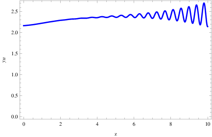
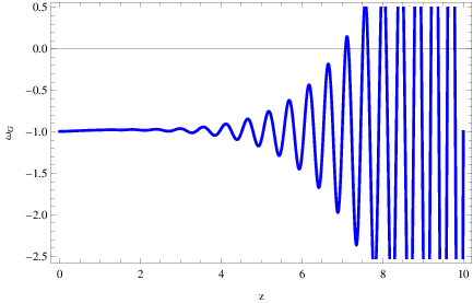
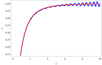
The parameters and will be assumed to take the values and . The phenomenology of the model (29) without the early dark energy term is quite interesting and is studied in detail in Odintsov:2020nwm, however we shall briefly show that it indeed yields a viable phenomenology at late-times. Then we shall include the early dark energy term in order to investigate when the early dark energy term affects the late-time era, and then constrain the parameter . For our late-time era analysis, we shall express all the quantities involved in the cosmological equations as functions of the redshift ,
| (38) |
by also taking the scale factor of the current Universe at equal to unity. Moreover, we introduce the statefinder quantity Hu:2007nk; Bamba:2012qi, which is equal to,
| (39) |
so by using the first Friedmann equation (30), takes the following form,
| (40) |
Due to the fact that , which means , with , and , is equal to,
| (41) |
We can easily express the Friedmann equations in terms of , so it reads Bamba:2012qi,
| (42) |
with the functions , and being defined in the following way,
| (43) |
with . We shall numerically solve the differential equation (42), in the redshift interval with the initial conditions for the function at redshift chosen as follows,
| (44) |
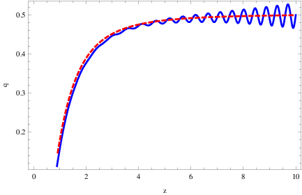
Let us now present the results of the numerical analysis, focusing first briefly on the model (29) without the presence of the early dark energy term. The full analysis of this model is performed elsewhere Odintsov:2020nwm. In order to have some standard comparison reference, we shall compare the results of the model (29) without the early dark energy term, with the CDM model. Accordingly, we shall compare the model without the early dark energy term, with the model (29), in the presence of the early dark energy term, in order to see which values of the parameter can affect the late-time behavior. Let us start off our analysis with the phenomenology of the model (29) without the early dark energy term, and by numerically solving the differential equation (42), we present the solution in the left plot of Fig. 1. In the right plot of Fig. 1, we present the dark energy EoS parameter , and in the bottom plot we present the deceleration parameter . In all the plots, the blue curves correspond to the gravity model (29) without the early dark energy term, and the red curves correspond to the CDM model. Also at , the value of the dark energy EoS parameter is evaluated to be , and also the dark energy density parameter is , which are within the constraints of the latest Planck data on the cosmological parameters. Moreover, the deceleration parameter is , which is very close to the CDM value . These results indicate that the model can be considered as phenomenologically viable.
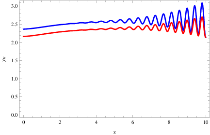
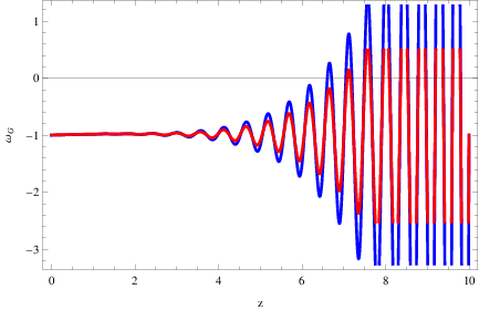
Now let us turn our focus on the model (29), by taking into account the presence of the early dark energy term. Since the early dark energy era is engineered to occur around the recombination era, so for , the curvature of the Universe at this era is of the order , we shall assume that . Also must be an odd integer in order for the early dark energy era to have an unstable de Sitter attractor, hence we take . Furthermore, and must be larger from , so we choose . As it seems, the early dark energy term has no effect on the late-time era, when , however, when , the early dark energy term starts to affect the late-time era. Indeed this can be seen in Fig. 2, where we plot the statefinder (left upper plot), the dark energy EoS parameter (right upper plot) and the deceleration parameter (bottom plot). In all the plots of Fig. 2, the blue curves correspond to the model (29), while the red curves to the model (29) without the early dark energy term. As it can be seen, the effects of the early dark energy term on the late-time evolution are significant, but this occurs only when . Also the value of the dark energy EoS parameter is , the dark energy density parameter and the deceleration parameter , so the effect of the early dark energy term affect the late-time dynamics for .
Another important issue to discuss in the matter density perturbations issue and the corresponding growth factor. In fact, the matter density perturbations can be considered as a consistent criterion that can distinguish the cosmic evolution corresponding to different gravities. This is because the cosmological matter density perturbations actually make possible the distinction between the evolution of each gravity from the background Matsumoto:2011ne. With regard to the matter density perturbations, a consistent calculation of these requires the subhorizon approximation, so that the theoretical framework is consistent with the Newtonian gravity Matsumoto:2011ne. The subhorizon approximation is quantified by the condition,
| (45) |
where is the scale factor and is the wavenumber of the comoving mode. Practically, the subhorizon approximation indicates that we should consider comoving wavelengths of a comoving mode , which are much shorter than the corresponding Hubble radius . The subhorizon approximation holds true during the matter domination era, and we shall focus on the last stage of the matter domination era and the dawn of the dark energy era, so for redshifts . The matter density perturbations are quantified by the parameter , which satisfies the following differential equation Bamba:2012qi,
| (46) |
where is the effective gravitational constant of the gravity theory, with its analytic form being for gravity Bamba:2012qi,
| (47) |
and denotes the present value of Newton’s constant of gravity. In the following we shall focus on the growth factor , so we can express the differential equation governing the matter density perturbations evolution (46) in terms of the growth factor. By using the following rules,
| (48) |
we can express the differential equation that governs the evolution of the matter perturbations (46), in terms of the growth factor,
| (49) |
From the above equation it is apparent that the effect of gravity on the growth factor is quantified in the term , and it is notable that the latter depends on the comoving wavenumber . By taking the present time Universe , the comoving number can be constrained by the present time value of the Hubble rate, so since , the wavenumber must be . In the following we shall numerically solve the differential equation (49), and we shall investigate two main issues, firstly the general behavior of the growth factor as a function of the redshift for various allowed values of the comoving wavenumber , for the model (21). Accordingly, we shall consider the model (29) in which the early dark energy term is added, and we shall investigate the behavior of the model and examine whether the early dark energy term affects the late-time behavior of the growth factor. This study shall validate the assumptions made in the previous late-time study, which indicated that when , the early dark energy term has no effect on the late-time evolution. For the numerical study, we shall assume that the growth factor at a redshift is equal to, Bamba:2012qi, which is the value of the growth factor for the CDM model. For comparison reasons, we shall also compare the gravity model (21) without the early dark energy term with the CDM, so at this point we quote the CDM expression for the growth factor, which is Basilakos:2012ws,
| (50) |
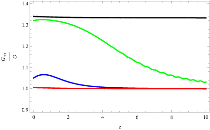
where in this case is the CDM model Hubble rate. Our aim at this point is to firstly indicate explicitly that the gravity model of Eq. (21) behaves similarly to the CDM model, and secondly, to investigate if the addition of the early dark energy era term affects the late-time behavior, and to which extent, having in mind that when the early dark energy term does not affect the late-time era, as we saw in the previous section. Let us first focus on the model (21) and in Fig. 3 we present the behavior of the fraction for (black curve), (green curve), (blue curve) and (red curve). As it can be seen, as the limiting allowed value is reached (red and blue curves), the effective gravitational constant approaches the present day Newton’s value.
Also in Fig. 4 we present the results of the numerical solution to the equation (49) which yields the growth factor as a function of the redshift, for (black curve), (blue curve), (green curve) and (yellow curve). Also the black dashed curve corresponds to the growth factor of the CDM model. As it can be seen, the green and yellow curves are indistinguishable from the CDM model, and deviations occur only for higher values of the wavenumber.
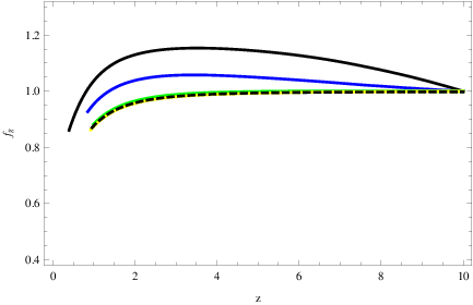
The results of the numerical analysis hold true, even when the early dark energy term is added, hence even for the model (29) and remarkably, no deviations occur even when . Therefore in conclusion, the dark energy era of the model (29) is not affected at all from the early dark energy term. Using the same approach as in this section, with similar a form of early dark energy, one can show that the realistic gravities unifying inflation with dark energy of Refs. Nojiri:2017ncd; Nojiri:2007as; Nojiri:2007cq; Cognola:2007zu; Nojiri:2006gh; Appleby:2007vb; Elizalde:2010ts; Odintsov:2020nwm, may be easily extended by adding an early dark energy term which does not spoil the inflationary and dark energy behavior of the models. For relevant works in the same unification of inflation with dark energy line of research see for example Benisty:2017lmt; Banerjee:2019kgu; Benisty:2019jqz.
A natural question that springs to mind is whether it is possible to obtain any new viable condition of gravity as an alternative gravity theory to general relativity? In principle, in the numerical study mainly, we investigated the constraints on the model (29) imposed by the requirement of the realization of the early dark energy era, in conjunction with the requirement that a viable late-time era is realized by the same model. As we showed, these two requirements severely constrained the values of the parameters , and .
At this point, let us comment on the two approaches we used in order to realize an early dark energy era. In the first approach, we used a rather quantitative method, which can provide the exact form of which reproduces an appropriately chosen phenomenological functional form of the Hubble rate. In this way, we can find the functional form of gravity, which reproduces a particular behavior of the Hubble rate in specific era, like matter dominated era, radiation dominated era, or dark energy dominated era and so on. In the second approach, however, we do not specify the Hubble rate, so it is analytically difficult to solve the equations of motion for a specifically chosen gravity. To be more specific in the first approach, the functional form of the Hubble rate is given, and one seeks the exact form of the gravity which may realize the appropriately chosen phenomenological Hubble rate. In the second approach, the phenomenology of various gravities containing terms that may realize an early dark energy is checked, but in this case numerically.
IV Conclusions
In this paper we investigated how a post-inflationary early dark energy era can be realized by gravity, and how to describe the inflationary era, the early and late-time dark energy era with a single gravity model. For our study we used two approaches, namely a quantitative approach in which we used a well-known reconstruction technique in order to realize a generalized Hubble rate that describes all the above mentioned cosmological eras. In our second approach, we used several qualitative arguments in order to construct an appropriate gravity that may realize inflation with the early and late-time dark energy eras. In the process of selecting a suitable early dark energy term, we investigated the constraints that the free parameters of the model must satisfy in order for an early dark energy era to be realized. Moreover, for one of the proposed models, we investigated the cosmological behavior of the model at late times, with and without the early dark energy term. We numerically integrated the Friedmann equation, by using the redshift as variable, and we expressed all the physical quantities as functions of the statefinder function , which solely depends on the redshift and the Hubble rate . The results of our numerical analysis indicated that the model is very similar to the CDM model at late-times, and also we demonstrated which values of the free parameters make the early dark energy term to have no effect on the late-time dark energy era. Also we investigated the behavior of the growth factor for the same model, and of the effective gravitational constant focusing on redshifts . For all the cases we studied, we found that the early dark energy term does not affect at all neither the effective gravitational constant, nor the growth factor. With regard to the effective gravitational constant, we found that for some values of the wavenumber, the gravitational constant is equal to the present time value of Newton’s gravitational constant, however, there are differences for a limited set of values of the wavenumber, mainly large values. This study should be extended to even larger redshifts, and this in principle could have an observable effect on the CMB, via the gravitational interaction and the Thomson scattering when the CMB was generated, exactly on the last scattering surface. In general the pivot scale dependence of cosmological parameters is a quite confusing issue in modern theoretical cosmology, so caution is required on this topic, therefore we did not go deeper in our analysis. In addition, with regard to the growth factor, since the latter characterizes the growth of the matter perturbations, an important quantity is the so-called growth index , which relates the growth factor with the matter density parameter as . The form of the growth index is currently unknown, and its value cannot be determined directly, however, its value may be inferred by the observational values of and . A cosmographic approach Benetti:2019gmo may also shed some light on the exact functional form of the growth index, but we defer this study to a future work.
Acknowledgments
This work is supported by MINECO (Spain), FIS2016-76363-P, and by project 2017 SGR247 (AGAUR, Catalonia) (S.D.O). This work is also supported by MEXT KAKENHI Grant-in-Aid for Scientific Research on Innovative Areas “Cosmic Acceleration” No. 15H05890 (S.N.) and the JSPS Grant-in-Aid for Scientific Research (C) No. 18K03615 (S.N.).
References
- (1) A. R. Liddle and D. H. Lyth, Cambridge, UK: Univ. Pr. (2000) 400 p
- (2) K. Aylor, M. Joy, L. Knox, M. Millea, S. Raghunathan and W. L. K. Wu, Astrophys. J. 874 (2019) no.1, 4 doi:10.3847/1538-4357/ab0898 [arXiv:1811.00537 [astro-ph.CO]].
- (3) K. C. Wong et al., arXiv:1907.04869 [astro-ph.CO].
- (4) L. Verde, T. Treu and A. G. Riess, Nature Astronomy 2019 doi:10.1038/s41550-019-0902-0 [arXiv:1907.10625 [astro-ph.CO]].
- (5) L. Knox and M. Millea, arXiv:1908.03663 [astro-ph.CO].
- (6) N. Aghanim et al. [Planck Collaboration], arXiv:1807.06209 [astro-ph.CO].
- (7) A. G. Riess et al., Astrophys. J. 826 (2016) no.1, 56 doi:10.3847/0004-637X/826/1/56 [arXiv:1604.01424 [astro-ph.CO]].
- (8) K. Migkas and T. H. Reiprich, Astron. Astrophys. 611 (2018) A50 doi:10.1051/0004-6361/201731222 [arXiv:1711.02539 [astro-ph.CO]].
- (9) M. E. Ramos-Ceja, F. Pacaud, T. H. Reiprich, K. Migkas, L. Lovisari and G. Schellenberger, Astron. Astrophys. 626 (2019) A48 doi:10.1051/0004-6361/201935111 [arXiv:1904.10275 [astro-ph.GA]].
- (10) M. Doran and G. Robbers, JCAP 0606 (2006) 026 doi:10.1088/1475-7516/2006/06/026 [astro-ph/0601544].
- (11) A. Bhattacharyya and S. Pal, arXiv:1907.10946 [astro-ph.CO].
- (12) J. Sakstein and M. Trodden, arXiv:1911.11760 [astro-ph.CO].
- (13) S. X. Tian, arXiv:1912.13208 [astro-ph.CO].
- (14) S. Nojiri, S. D. Odintsov and V. K. Oikonomou, Phys. Rept. 692 (2017) 1 doi:10.1016/j.physrep.2017.06.001 [arXiv:1705.11098 [gr-qc]].
- (15) S. Nojiri, S. D. Odintsov and D. Saez-Gomez, Phys. Lett. B 681 (2009) 74 doi:10.1016/j.physletb.2009.09.045 [arXiv:0908.1269 [hep-th]].
- (16) S. Capozziello and M. De Laurentis, Phys. Rept. 509 (2011) 167 doi:10.1016/j.physrep.2011.09.003 [arXiv:1108.6266 [gr-qc]].
- (17) V. Faraoni and S. Capozziello, Fundam. Theor. Phys. 170 (2010). doi:10.1007/978-94-007-0165-6
- (18) S. Nojiri and S. D. Odintsov, eConf C 0602061 (2006) 06 [Int. J. Geom. Meth. Mod. Phys. 4 (2007) 115] doi:10.1142/S0219887807001928 [hep-th/0601213].
- (19) S. Nojiri and S. D. Odintsov, Phys. Rept. 505 (2011) 59 doi:10.1016/j.physrep.2011.04.001 [arXiv:1011.0544 [gr-qc]].
- (20) A. de la Cruz-Dombriz and D. Saez-Gomez, Entropy 14 (2012) 1717 doi:10.3390/e14091717 [arXiv:1207.2663 [gr-qc]].
- (21) G. J. Olmo, Int. J. Mod. Phys. D 20 (2011) 413 doi:10.1142/S0218271811018925 [arXiv:1101.3864 [gr-qc]].
- (22) S. Capozziello, Int. J. Mod. Phys. D 11 (2002) 483 doi:10.1142/S0218271802002025 [gr-qc/0201033].
- (23) S. M. Carroll, V. Duvvuri, M. Trodden and M. S. Turner, Phys. Rev. D 70 (2004) 043528 doi:10.1103/PhysRevD.70.043528 [astro-ph/0306438].
- (24) S. Nojiri and S. D. Odintsov, Phys. Rev. D 68 (2003) 123512 doi:10.1103/PhysRevD.68.123512 [hep-th/0307288].
- (25) S. Nojiri and S. D. Odintsov, Phys. Lett. B 657 (2007) 238 doi:10.1016/j.physletb.2007.10.027 [arXiv:0707.1941 [hep-th]].
- (26) S. Nojiri and S. D. Odintsov, Phys. Rev. D 77 (2008) 026007 doi:10.1103/PhysRevD.77.026007 [arXiv:0710.1738 [hep-th]].
- (27) G. Cognola, E. Elizalde, S. Nojiri, S. D. Odintsov, L. Sebastiani and S. Zerbini, Phys. Rev. D 77 (2008) 046009 doi:10.1103/PhysRevD.77.046009 [arXiv:0712.4017 [hep-th]].
- (28) S. Nojiri and S. D. Odintsov, Phys. Rev. D 74 (2006) 086005 doi:10.1103/PhysRevD.74.086005 [hep-th/0608008].
- (29) S. A. Appleby and R. A. Battye, Phys. Lett. B 654 (2007) 7 doi:10.1016/j.physletb.2007.08.037 [arXiv:0705.3199 [astro-ph]].
- (30) E. Elizalde, S. Nojiri, S. D. Odintsov, L. Sebastiani and S. Zerbini, Phys. Rev. D 83 (2011) 086006 doi:10.1103/PhysRevD.83.086006 [arXiv:1012.2280 [hep-th]].
- (31) S. D. Odintsov and V. K. Oikonomou, arXiv:2001.06830 [gr-qc].
- (32) S. D. Odintsov and V. K. Oikonomou, Phys. Rev. D 99 (2019) no.10, 104070 doi:10.1103/PhysRevD.99.104070 [arXiv:1905.03496 [gr-qc]].
- (33) S. D. Odintsov and V. K. Oikonomou, Phys. Rev. D 99 (2019) no.6, 064049 doi:10.1103/PhysRevD.99.064049 [arXiv:1901.05363 [gr-qc]].
- (34) G. Bertone, D. Hooper and J. Silk, Phys. Rept. 405 (2005) 279 doi:10.1016/j.physrep.2004.08.031 [hep-ph/0404175].
- (35) L. Bergstrom, Rept. Prog. Phys. 63 (2000) 793 doi:10.1088/0034-4885/63/5/2r3 [hep-ph/0002126].
- (36) Y. Mambrini, S. Profumo and F. S. Queiroz, Phys. Lett. B 760 (2016) 807 [arXiv:1508.06635 [hep-ph]].
- (37) S. Profumo, arXiv:1301.0952 [hep-ph].
- (38) D. Hooper and S. Profumo, Phys. Rept. 453 (2007) 29 [hep-ph/0701197].
- (39) V. K. Oikonomou, J. D. Vergados and C. C. Moustakidis, Nucl. Phys. B 773 (2007) 19 [hep-ph/0612293].
- (40) S. Capozziello, S. Carloni and A. Troisi, Recent Res. Dev. Astron. Astrophys. 1 (2003) 625 [astro-ph/0303041].
- (41) S. Odintsov and V. Oikonomou, Class. Quant. Grav. 33 (2016) no.12, 125029 doi:10.1088/0264-9381/33/12/125029 [arXiv:1602.03309 [gr-qc]].
- (42) S. A. Appleby, R. A. Battye and A. A. Starobinsky, JCAP 1006 (2010) 005 doi:10.1088/1475-7516/2010/06/005 [arXiv:0909.1737 [astro-ph.CO]].
- (43) W. Hu and I. Sawicki, Phys. Rev. D 76 (2007) 064004 doi:10.1103/PhysRevD.76.064004 [arXiv:0705.1158 [astro-ph]].
- (44) K. Bamba, A. Lopez-Revelles, R. Myrzakulov, S. D. Odintsov and L. Sebastiani, Class. Quant. Grav. 30 (2013) 015008 doi:10.1088/0264-9381/30/1/015008 [arXiv:1207.1009 [gr-qc]].
- (45) J. Matsumoto, Phys. Rev. D 83 (2011) 124040 doi:10.1103/PhysRevD.83.124040 [arXiv:1105.1419 [astro-ph.CO]].
- (46) S. Basilakos, Int. J. Mod. Phys. D 21 (2012) 1250064 doi:10.1142/S0218271812500642 [arXiv:1202.1637 [astro-ph.CO]].
- (47) D. Benisty and E. I. Guendelman, Int. J. Mod. Phys. A 33 (2018) no.20, 1850119 doi:10.1142/S0217751X18501191 [arXiv:1710.10588 [gr-qc]].
- (48) S. Banerjee, D. Benisty and E. I. Guendelman, arXiv:1910.03933 [gr-qc].
- (49) D. Benisty, E. I. Guendelman, E. N. Saridakis, H. Stoecker, J. Struckmeier and D. Vasak, Phys. Rev. D 100 (2019) no.4, 043523 doi:10.1103/PhysRevD.100.043523 [arXiv:1905.03731 [gr-qc]].
- (50) M. Benetti and S. Capozziello, arXiv:1910.09975 [astro-ph.CO].