跳到论文正文
W Papers独立论文阅读器 arXiv:1912.13028 论文正文 计算阅读时间 · 0%
引用这篇论文根据当前论文元数据生成,正式投稿前建议核对。


License: arXiv.org perpetual non-exclusive license
arXiv:1912.13028v1 [cond-mat.mes-hall] 30 Dec 2019

Thermal signature of Majorana fermions in Josephson junction

Aabir Mukhopadhyay Email: aabir.riku@gmail.com Affiliation: Indian Institute of Science Education & Research Kolkata, Mohanpur, Nadia - 741 246, West Bengal, India    Sourin Das Email: sourin@iiserkol.ac.in,
ORCID ID : 0000-0002-8511-5709
Affiliation: Indian Institute of Science Education & Research Kolkata, Mohanpur, Nadia - 741 246, West Bengal, India
August 11, 2026
Abstract

Existence of distinctive correlation between the thermal conductance and the Josephson current across a 1-D topological Josephson junction (T-JJ) is established and an expression connecting the two is derived in the short junction limit. It is shown that the three terminal T-JJ provides us with an ideal set-up for exploiting the distinctive correlations which aid in identifying hallmarks of Majorana bound state localized at the junction. Our approach combines information form sub-gap Cooper pair transport and transport of above-gap thermally excited quasiparticle which is complementary to the existing studies.

Introduction: Maki and GriffinMaki and Griffin 1965; Maki and Griffin 1966 carried out theoretical study of heat transport across a Josephson junction (JJ) in 1965 and ever since there have been several studies pertaining to thermal transport across JJsGuttman et al. 1997; Zhao et al. 2003; Zhao et al. 2004; Fornieri et al. 2017; Luo et al. 2019 including some recent developments involving two and three dimensional topological insulatorsSothmann and Hankiewicz 2016; Sothmann et al. 2017. On the experimental side, the theoretical predictionsMaki and Griffin 1965; Maki and Griffin 1966 were confirmed in a remarkable experiment by Giazotto and Martinez-Perez in 2012Giazotto and Martínez-Pérez 2012 which led to steady experimental progress in this fieldGolubev et al. 2013; Martínez-Pérez and Giazotto 2013; Martínez-Pérez et al. 2014; Martínez-Pérez and Giazotto 2014; Martínez-Pérez et al. 2015; Fornieri et al. 2016a; Kolenda et al. 2016; Fornieri et al. 2016b; Tan et al. 2017; Fornieri and Giazotto 2017; Paolucci et al. 2018; Karimi and Pekola 2018.
Proximity induced superconductivity in spin-orbit nano-wire and the helical edge state (HES) of quantum spin Hall (QSH) state allow for two distinct realizations of topological superconductivity and localized Majorana bound states (MBS)Lutchyn et al. 2010; Oreg et al. 2010; Nadj-Perge et al. 2010; Liang and Gao 2012; Mourik et al. 2012; Das et al. 2012; Sestoft et al. 2018; Bommer et al. 2019; König et al. 2007; Brüne et al. 2010; Knez et al. 2011; Brüne et al. 2012; Knez et al. 2012; Hart et al. 2014. In case of a nano-wire, these MBS are expected to appear at the two ends of the wireKitaev 2001 while for Helical edge state (HES) of QSE state, localized MBS forms at the junction of a proximity induced superconducting region and a region exposed to Zeeman fieldFu and Kane 2009; Nilsson et al. 2008. It is pertinent to note that experimental realization of T-JJs11 1 Topological JJ refers to those JJ where the sub-gap bound state formed at the junction are primarily due to overlap of Majorana bound state appearing at the ends of the topological supercondcutors. has been achieved both in the context of nano-wire set-upLaroche et al. 2019 and HEH of QSE state set-upBocquillon et al. 2017. These experimental advances call for a renewed look at how to exploit a combination of electrical and thermal means to detect and manipulate the MBS.

As far as detection of MBS via Josephson effect is concerned, observation of 4​π4\pi Josephson effectKwon et al. 2004; Fu and Kane 2009 is considered as a hallmark of MBS which primarily relates to sub-gap physics. The central focus of this article is to establish that the above-gap transport of thermally excited bulk quasi-particle (Q​PQP) across a JJ also carry distinctive signatures of topological superconductivity and MBS. This can be understood as follows.
It is known that the thermal current across a JJ in the weak tunneling limit can be expressed as a sum of contribution due to Q​PQPs tunneling, Cooper pairs tunneling (which is usually negligiblePershoguba and Glazman 2019) and the interference of the twoMaki and Griffin 1965; Maki and Griffin 1966; Guttman et al. 1998. For a JJ with arbitrary transparency, these interferences simply lead to zero in denominator of transmission probability of Q​P​sQPs at energies (denoted by ω0\omega_{0}) at which Andreev bound state (ABS)Sauls 2018; Beenakker 1991; Octavio et al. 1983; Bardeen et al. 1969 are formed in the JJ. Remarkably, the phase bias (ϕ\phi) of 1-D T-JJ enters the Q​PQP transmission probability solely via the dependence of sub-gap bound states energy(ω0​(ϕ)\omega_{0}(\phi)) on ϕ\phi. In contrast, the ϕ\phi dependence of a 1-D non-topological JJ appears also in the numerator of the Q​PQP transmission probability resulting in a complicated function of ϕ\phi (see Appendix A). Recall that the Josephson current is dominated by contributions from ϕ\phi derivative of the sub-gap bound state energy, ω0​(ϕ)\omega_{0}(\phi) in the short junction limitBeenakker 1991. Hence, the ϕ\phi dependence of both the heat current carried by the thermally excited Q​PQP and Josephson current carried by Cooper pairs acquire their ϕ\phi dependence primarily from their dependence on ω0​(ϕ)\omega_{0}(\phi), leading to a distinctive correlation between the two independently measurable quantities. An additional correlation which exists on a similar footing as ϕ\phi arises via the dependence of sub-gap bound state energy (ω0\omega_{0}) on the normal state transmission probability (τ\tau). In what follows, we will focus on the short JJ limit unless stated otherwise.
We study correlation between Josephson current, thermal conductance and the corresponding normal state electrical conductance of a three terminal T-JJ as a function of (ϕ\phi,τ\tau). We derive a set of relations (see Eq.[11] and Eq.[12]) between these quantities. The validity of these relations owes its existence to the presence of MBS at the junction and therefore is a smoking gun signature of MBS. We stress that the three terminal T-JJ set-up is expected to host a single MBS pinned at zero energy22 2 This is so because each topological superconductor will contribute a single Majorana to the Josephson tri-junction but two of them will hybridize and gap out while the third MBS will stay topologically protected. and therefore is of particular importance as a testing ground for MBS. Note that a study involving thermal conductance of topological ABS was reported in Ref.[Sothmann and Hankiewicz 2016] though it did not touch upon the ideas presented here, i.e., the detection of MBS using a multi-terminal set-up or correlation between electrical and thermal response of T-JJ.
Multi-terminal thermal conductance: For a multi-terminal junction, heat currents driven by temperature bias within linear response theory can be expressed as

Inh=∑m≠nκn,m​(Tn−Tm)I^{h}_{n}=\sum_{m\neq n}\kappa_{n,m}(T_{n}-T_{m}) (1)

where κn,m\kappa_{n,m} is the thermal conductance between terminal mm, nn and TnT_{n}, TmT_{m} are the temperatures of terminal nn and mm respectively. We consider a general multi-terminal junction of superconducting leads (described by BdG HamiltonianDe Gennes 2018) connected via a common normal region. An incident electron-like quasiparticle in mmth lead (with energy ω\omega) results in a reflected electron-like and hole-like quasiparticle within the same lead with probabilities, say ℛe,em,m\mathcal{R}^{m,m}_{e,e} and ℛh,em,m\mathcal{R}^{m,m}_{h,e} respectively along with transmitted electron-like and hole-like quasiparticle in the nnth lead (n≠m)(n\neq m) with probabilities 𝒯e,en,m\mathcal{T}^{n,m}_{e,e} and 𝒯h,en,m\mathcal{T}^{n,m}_{h,e} respectively. Probability conservation ensures that (ℛe,em,m+ℛh,em,m)+∑n(𝒯e,en,m+𝒯h,en,m)=1(\mathcal{R}^{m,m}_{e,e}+\mathcal{R}^{m,m}_{h,e})+\sum_{n}(\mathcal{T}^{n,m}_{e,e}+\mathcal{T}^{n,m}_{h,e})=1. We denote 𝒯n,m=𝒯en,m+𝒯hn,m=(𝒯e,en,m+𝒯h,en,m)+(𝒯h,hn,m+𝒯e,hn,m)\mathcal{T}^{n,m}=\mathcal{T}^{n,m}_{e}+\mathcal{T}^{n,m}_{h}=(\mathcal{T}^{n,m}_{e,e}+\mathcal{T}^{n,m}_{h,e})+(\mathcal{T}^{n,m}_{h,h}+\mathcal{T}^{n,m}_{e,h}). The multi-terminal linear response thermal conductance between leads mm and nn is then given by Sothmann and Hankiewicz 2016

κn,m​(ϕj)=[1h​∫Δ0∞d​ω​ω​{𝒯n,m}​d​f​(ω,T)d​T]T=Tavg,\kappa_{n,m}(\phi_{j})=\left[\,\dfrac{1}{h}\int_{\Delta_{0}}^{\infty}d\omega\,\omega\,\{\mathcal{T}^{n,m}\}\dfrac{df(\omega,T)}{dT}\right]_{T=T_{\text{avg}}}, (2)

where f⁡(ω,T)f(\omega,T) is the Fermi distribution function at temperature TT, Δ0\Delta_{0} is the superconducting gap (taken to be same of all leads) and TavgT_{\text{avg}} is the average junction temperature.
Two Terminal T-JJ in HES: Though our findings are valid for 1-D T-JJ based on either (a) 1-D electrons with quadratic dispersion and proximitized p-wave superconductivityDeb et al. 2018 or (b) 1-D Dirac fermions with proximitized s-wave superconductivity, we will primarily discuss the case of 1-D Dirac fermions realized in HES of QSH state. We consider a JJ in HES where the junction is defined by |x|<L/2|x|<L/2 region and we have a finite pair potential Δ0​ei​ϕr\Delta_{0}e^{i\phi_{r}} ([r∈{1,2}][r\in\{1,2\}]) for ∞>|x|>L/2\infty>|x|>L/2 (see Fig[1] (a)). Our set-up is described by Bogoliubov-de Gennes HamiltonianFu and Kane 2009; Dolcini et al. 2015 in the Nambu basis (Ψ=[(ψ↑,ψ↓),(ψ↓†,−ψ↑†)]T\Psi=[(\psi_{\uparrow},\psi_{\downarrow}),(\psi_{\downarrow}^{\dagger},-\psi_{\uparrow}^{\dagger})]^{T}(Fu and Kane 2008)) given by

ℋ=(vF​p^x​σz−μ)​τz+Δ⁡(x)​(cos⁡ϕr​τx−sin⁡ϕr​τy),\displaystyle\mathcal{H}=(v_{F}\hat{p}_{x}\sigma_{z}-\mu)\uptau_{z}+\Delta(x)(\cos\phi_{r}\uptau_{x}-\sin\phi_{r}\uptau_{y}), (3)

where Δ⁡(x)=Δ0​[Θ⁡(−x−L/2)+Θ⁡(x−L/2)]\Delta(x)=\Delta_{0}[\Theta(-x-L/2)+\Theta(x-L/2)], σ\sigma and τ\uptau represents spin and particle-hole degrees of freedom respectively. We focus on the highly doped regime given by the chemical potential μ>>Δ0\mu>>\Delta_{0} and at the short junction limit given by L<<ξL<<\xi, where ξ=ℏ​vF/Δ0\xi=\hbar v_{F}/\Delta_{0} is the superconducting coherence length. For ω<Δ0\omega<\Delta_{0} (measured with respect to μ\mu) Andreev bound states (ABS) are formed at energy ω0±=±Δ0τcosϕ/2\omega_{0}^{\pm}=\pm\Delta_{0}\sqrt{\tau}\cos\phi/2 (ϕ=ϕ2−ϕ1)(\phi=\phi_{2}-\phi_{1}) (see Supplemental Material: Section A) while for ω>Δ0\omega>\Delta_{0} we have propagating quasiparticle solutions. Here τ\tau represents transmission probability scattering matrix SS introduced at x=0x=0 and is assumed to be energy independent. The quasiparticle transmission probability across the JJ described by Eq.[A1], 𝒯1,2\mathcal{T}^{1,2}, can be expressed as (see Supplemental Material: Section A)

𝒯1,2​(ω,τ,ϕ)=τ⁡[2​(ω2−Δ02)​𝔣​(ω,τ,ϕ)(ω2−|ω0±​(τ,ϕ)|2)2]​Θ​(|ω|2−Δ02),\mathcal{T}^{1,2}(\omega,\tau,\phi)=\tau~\left[\dfrac{2\,(\omega^{2}-\Delta_{0}^{2})\,\mathfrak{f}(\omega,\tau,\phi)}{(\omega^{2}-|\omega_{0}^{\pm}(\tau,\phi)|^{2})^{2}}\right]\,\Theta(|\omega|^{2}-\Delta_{0}^{2})\,, (4)
Refer to caption
Figure 1: (a) Pictorial representation of two-terminal JJ hosted on HES where a backscatterer SS is introduced at x=0x=0. (b) Plot of thermal conductance κ\kappa for ϕ=0\phi=0 in units of GQG_{Q} is plotted as a function of τ\tau for a normal junction (non-superconducting) and the corresponding non-topological and topological JJ at ϕ=0\phi=0. (c) Three dimensional surface plot of difference between topological and non-topological case in the (1CLOSE(1-OPENτ)\tau)-(kB​Tavg/Δ0)(k_{B}T_{\text{avg}}/\Delta_{0}) plane.

which is general form for 𝒯\mathcal{T} in case of 1-D JJ in the short junction limit. For the T-JJ, 𝔣⁡(ω,τ,ϕ)=(ω2−|ω0±​(τ,ϕ)|2)\mathfrak{f}(\omega,\tau,\phi)=(\omega^{2}-|\omega_{0}^{\pm}(\tau,\phi)|^{2}), which cancels with its square appearing in the denominator and hence leading to a ϕ\phi dependence of 𝒯\mathcal{T} solely via the ϕ\phi dependence of energy of ABS (ω0±\omega_{0}^{\pm}) appearing in the denominator. Also the τ\tau dependence of 𝒯\mathcal{T} enters solely via ω0​(τ,ϕ)\omega_{0}(\tau,\phi) except for the expected overall multiplicative dependence on τ\tau as shown in R.H.S of Eq.[4]. In contrast, for the non-topological JJ, 𝔣⁡(ω,τ,ϕ)=(ω2−Δ02​cos⁡ϕ−τ​Δ02​sin2​ϕ/2)\mathfrak{f}(\omega,\tau,\phi)=(\omega^{2}-\Delta_{0}^{2}\cos\phi-\tau\Delta_{0}^{2}\sin^{2}\phi/2) (Zhao et al. 2003; Zhao et al. 2004) which leads to a complicated (ϕ\phi, τ\tau) dependence of 𝒯\mathcal{T}. We will show the above discussed observations pave the way to identification of distinctive correlation between electrical and thermal currents of a three terminal T-JJ which carry signatures of isolated MBS localized at the junction.
Signatures of topological ABS in two-terminal thermal conductance : We first discuss signature of the T-JJ pertaining to its τ\tau dependence in thermal conductance in the simplest case of ϕ=0\phi=0. For a non-topological JJ, 𝒯1,2​(ω,τ,ϕ=0)=2​τ\mathcal{T}^{1,2}(\omega,\tau,\phi=0)=2\,\tau (see Appendix A), thus the thermal conductance of such a JJ in the absence of phase bias is given by (using Eq.A15) κ=2​τ​[GQ−∫0Δ0d​ω​ω​𝑑f​(ω,T)/𝑑T]T=Tavg\kappa=2\,\tau[G_{Q}-\int_{0}^{\Delta_{0}}d\omega\,\omega df(\omega,T)/dT]_{T=T_{\text{avg}}} where GQ=π2​kB2​T/(3​h)G_{Q}=\pi^{2}k_{B}^{2}T/(3h) is quantized thermal conductance of a single ballistic channel and the factor of 22 represents the doubling due to contributions from particle and hole channels. Hence it equals two times the normal state thermal conductance suppressed up to the gap(Zhao et al. 2003; Zhao et al. 2004) (see Fig.[1] (b)). But for the T-JJ, 𝒯1,2​(ω,τ,ϕ=0)=2​τ​(1−α)\mathcal{T}^{1,2}(\omega,\tau,\phi=0)=2\,\tau(1-\alpha) where α=Δ02​((1−τ)/(ω2−τ​Δ02))\alpha=\Delta_{0}^{2}((1-\tau)/(\omega^{2}-\tau\Delta_{0}^{2})), which implies an additional suppression proportional to α\alpha w.r.t. the non-topological JJ. This contrast between topological and non-topological case stem from the fact that at zero phase bias ( ϕ=0\phi=0 ) the ABS energy stays pined at ω0±=±Δ0\omega_{0}^{\pm}=\pm\,\Delta_{0} and hence is independent of transmissivity (τ\tau) of the junction for non-topological case. On the contrary the ABS energy |ω0±|<Δ0|\omega_{0}^{\pm}|<\Delta_{0} for the topological case when ϕ=0\phi=0 and its exact value depends on τ\tau. Hence this additional suppression of thermal conductance of T-JJ for at ϕ=0\phi=0 (see Fig.[1], (c)) is a direct manifestation of topological ABS.

Refer to caption
Figure 2: Pictorial representation of an effective three terminal JJ depicted on HES of QSH bar geometry where SS represent scattering at x=0x=0 due to the QPC. M​σ⟂M\sigma_{\perp} represents an local magnetic field perpendicular to the spin-quantization axis of HES.

Now we start focusing on quantifying the correlation between κ\kappa and Josephson current discussed above. From (A15) and (4) we note that the thermal conductance of a T-JJ can be expressed as

κ=σN​[2e2​β​(T)​∫Δ0∞d​ω​ω​(ω2−Δ02)(ω2−|ω0±|2​(τ,ϕ))​d​f​(ω,T)d​T]T=Tavg,\kappa=\sigma^{N}\left[\dfrac{2}{e^{2}\beta(T)}\int_{\Delta_{0}}^{\infty}d\omega\,\omega\dfrac{\,(\omega^{2}-\Delta_{0}^{2})}{(\omega^{2}-|\omega_{0}^{\pm}|^{2}(\tau,\phi))}\dfrac{df(\omega,T)}{dT}\right]_{T=T_{\text{avg}}}, (5)

where σN=(e2​τ/h)​β​(T)\sigma^{N}=(e^{2}\tau/h)\beta(T) is Landauer-Buttiker conductance Landauer 1957a; Moskalets 2011 at finite temperature where β(T)=∫−∞∞(−∂f/∂ω)dω=(4kBT)−1∫−∞∞[cosh⁡(ω2​kB​T)]−2dω\beta(T)=\int_{-\infty}^{\infty}(-\partial f/\partial\omega)d\omega=(4k_{B}T)^{-1}\int_{-\infty}^{\infty}\left[\cosh(\frac{\omega}{2k_BT})\right]^{-2}d\omega is the thermal broadening factor. We also note that the Josephson current (IJI^{J}) at temperature TT is given byBeenakker 1991

IJ=−2​eℏ​∂|ω0±|∂ϕ​tanh⁡(|ω0±|2​kB​T).I^{J}=-\dfrac{2e}{\hbar}\dfrac{\partial|\omega_{0}^{\pm}|}{\partial\phi}\tanh\left(\dfrac{|\omega_{0}^{\pm}|}{2k_{B}T}\right). (6)

Now it is straightforward to note that the Josephson current can be related to the corresponding thermal conductance of the T-JJ via the relation (see Supplemental Material: Section A)

∂ϕκ\displaystyle\partial_{\phi}\kappa =σN​IJ​[−h​|ω0±|π​e3​{1β⁡(T)​coth⁡(|ω0±|2​kB​T)}​∫Δ0∞d​ω​ω​ω2−Δ02(ω2−|ω0±|2)2​d​f​(ω,T)d​T]T=Tavg,\displaystyle=\sigma^{N}\,I^{J}\,\left[\dfrac{-h|\omega_{0}^{\pm}|}{\pi e^{3}}\bigg\{\frac{1}{\beta(T)}\coth\left(\dfrac{|\omega_{0}^{\pm}|}{2k_{B}T}\right)\bigg\}\int_{\Delta_{0}}^{\infty}d\omega\,\omega\dfrac{\omega^{2}-\Delta_{0}^{2}}{(\omega^{2}-|\omega_{0}^{\pm}|^{2})^{2}}\dfrac{df(\omega,T)}{dT}\right]_{T=T_{\text{avg}}}, (7)

which directly exploits the fact that the ϕ\phi dependence in both IJI^{J} and κ\kappa stem from ω0\omega_{0} dependence of ϕ\phi. We show next that that the three terminal thermal conductance also follows the same relation between ∂ϕk​lκi,j\partial_{\phi_{kl}}\kappa_{i,j} and corresponding σi,jN\sigma^{N}_{i,j}, Ii,jJI^{J}_{i,j} (i,j=1,2,3i,j=1,2,3) owing to the presence of topologically protected MBS at the tri-junction. This fact leads to the central finding of this letter presented in Eq.[11] and Eq.[12].
Three Terminal Topological JJ in HES: We consider a Hall bar (QSHB) geometry hosting a QSH state comprising of two helical states with opposite helicity at its opposite edges subjected to a quantum point contact(QPC) which enables us to design an effective four terminal topological JJ (Fig. [2]).We also apply a Zeeman filed pointing perpendicular to the spin-polarization axis (i.e. zz axis) along left half of the upper edge as shown in the Fig.[2] which open up a mass gap in the edge spectrum and reduces the set-up to a three terminal geometry.
Hence a three terminal JJ can be simulated by the following BdG Hamiltonian given by

ℋη=\displaystyle\mathcal{H}_{\eta}= He​d​g​e+Hg​a​p\displaystyle H_{edge}+H_{gap} (8)
=\displaystyle= {(ηvFp^xσz−μ)τz+\displaystyle\{(\eta v_{F}\hat{p}_{x}\sigma_{z}-\mu)\uptau_{z}+ Δ(x)(cosϕrτx−sinϕrτy)}\displaystyle\Delta(x)(\cos\phi_{r}\uptau_{x}-\sin\phi_{r}\uptau_{y})\}
+\displaystyle+ {(η−1)/2}​M​(x)​σ⟂\displaystyle\{(\eta-1)/2\}\,M(x)\sigma_{\perp}

subjected to a scattering matrix (SS) imposed at x=0x=0 that generates scattering between upper and lower edge (see Fig.[2]). We derived SS starting from a local tunnel Hamiltonian representing intra-edge tunneling at x=0x=0 in Supplemental Material (Section B) which is used for performing numerical analysis later on. Here η\eta defines the helicity of the edge state: η=1\eta=1 for lower edge and η=−1\eta=-1 for upper edge. Pairing potentials in the four superconducting terminals shown in Fig.[2] is given by Δ0​ei​ϕr\Delta_{0}e^{i\phi_{r}} where [r∈{1,2,3,4}][r\in\{1,2,3,4\}] and M⁡(x)=M0​Θ​(x+L/2)​Θ​(−x)M(x)=M_{0}\Theta(x+L/2)\Theta(-x) and M0→∞M_{0}\rightarrow\infty. Other notations has their usual meaning as described before. Assuming that SS is such that its elements respects, |(S)i,j|=|(S)j,i||(S)_{i,j}|=|(S)_{j,i}| (i,j=1,2,3i,j=1,2,3), the solutions for the sub-gap gap bound state (ω<Δ0\omega<\Delta_{0}) reduces to ω0= 0,±Δ0(τ12cos2ϕ122+τ23cos2ϕ232+τ13sin2ϕ132)1/2=ω00,ω0±\omega_{0}=\,0,\pm\,\Delta_{0}\left(\tau_{12}\cos^{2}\frac{\phi_{12}}{2}+\tau_{23}\cos^{2}\frac{\phi_{23}}{2}+\tau_{13}\sin^{2}\frac{\phi_{13}}{2}\right)^{1/2}=\omega_{0}^{0},\omega_{0}^{\pm} (see Supplemental Material: Section C) where ϕi​j=ϕj−ϕi\phi_{ij}=\phi_{j}-\phi_{i} 33 3 If arg⁡(S)i,j≠arg⁡(S)j,i\arg{(S)_{i,j}}\neq\arg{(S)_{j,i}} then the relative phase of the scattering matrix leads to a additive contribution to ϕi,j\phi_{i,j} leading to anomalous Josepson current. and τi​j=|(S0)i,j|2\tau_{ij}=|(S_{0})_{i,j}|^{2}. Insight into the form of sub-gap bound state solution can be obtained by considering an effective Majorana Hamiltonian where each superconducting terminal (i=1,2,3i=1,2,3) is expected to contribute one Majorana to the junction except the forth terminal where the Majorana has been pushed away owing to the Zeeman gap. The effective majorana Hamiltonian then takes the form,Fu and Kane 2009; Alicea 2012; Houzet and Meyer 2019

H=i2​∑1≤a≤b≤4ξa​b​γa​γb,H=\dfrac{i}{2}\sum_{1\leq a\leq b\leq 4}\xi_{ab}\gamma_{a}\gamma_{b}, (9)

where ξa​b=Δ02​τa​b​cos⁡(ϕa​b2−χa​b2)\xi_{ab}=\dfrac{\Delta_{0}}{2}\sqrt{\tau_{ab}}\cos\left(\frac{\phi_{ab}}{2}-\frac{\chi_{ab}}{2}\right) and γa\gamma_{a} is the Majorana zero mode operator corresponding to terminal a=1,2,3,4a=1,2,3,4 . We consider χi​i=χ13=χ24=π\chi_{ii}=\chi_{13}=\chi_{24}=\pi which incorporates the excess Berry phase due to spin flip scattering at the QPC. To mimic our three terminal situation we take ti​4=t4​i=0t_{i4}=t_{4i}=0 for i≠4i\neq 4 and hence ξ14=ξ24=ξ34=0\xi_{14}=\xi_{24}=\xi_{34}=0. This Majorana Hamiltonian readily provides two zero energy eigenvalues and the other two eigenvalues being identical to ω0±\omega_{0}^{\pm} given above. Note that three of these eigenstate corresponds to hybridised γ1\gamma_{1}, γ2\gamma_{2} and γ3\gamma_{3} resulting in an MBS that stays pinned to zero energy (ϵ=0\epsilon=0) and a pair of Andreev bound states at energy ϵ±=ω0±\epsilon_{\pm}=\omega_{0}^{\pm} while the fourth zero energy state corresponds to the MBS which stays isolated from the junction.
Now returning back to Hamiltonian in Eq.[8], for energies ω>Δ0\omega>\Delta_{0}, 𝒯i,j\mathcal{T}^{i,j}, the total quasiparticle transmission probability from terminal jj to terminal ii is given by (see Supplemental Material: Section D)

𝒯i,j​(ω,τi​j,ϕi​j)=\displaystyle\mathcal{T}^{i,j}(\omega,\tau_{ij},\phi_{ij})= τi​j​[2​(ω2−Δ02)​𝔣​(ω,τi​j,ϕi​j)∏ω0(ω−ω0​(τi​j,ϕi​j))2]\displaystyle\tau_{ij}\left[\dfrac{2(\omega^{2}-\Delta_{0}^{2})~\mathfrak{f}(\omega,\tau_{ij},\phi_{ij})}{\prod_{\omega_{0}}(\omega-\omega_{0}(\tau_{ij},\phi_{ij}))^{2}}\right] (10)
×Θ⁡(|ω|2−Δ02),\displaystyle\times\Theta(|\omega|^{2}-\Delta_{0}^{2}),

where [i,j∈{1,2,3},j>i][i,j\in\{1,2,3\},j>i] and 𝔣=ω2​(ω2−|ω0±|2)\mathfrak{f}=\omega^{2}(\omega^{2}-|\omega_{0}^{\pm}|^{2}). The resulting expression of 𝒯n,m\mathcal{T}^{n,m} has a perfect congruence with two terminal case (see Eq.[4]) due to cancellation of ω2\omega^{2} in the numerator with (ω−ω0​(τi​j,ϕi​j))ω0=ω002(\omega-\omega_{0}(\tau_{ij},\phi_{ij}))_{\omega_{0}=\omega_{0}^{0}}^{2} in the denominator owing to the MBS at ω0=ω00=0\omega_{0}=\omega_{0}^{0}=0. This similarity immediately validates Eq.[5] and Eq.[7] for the three terminal case also where κ→κi,j\kappa\rightarrow\kappa_{i,j}, ϕ→ϕi​j\phi\rightarrow\phi_{ij}, σN→σi,jN\sigma^{N}\rightarrow\sigma_{i,j}^{N} and IJ→Ii,jJI^{J}\rightarrow I^{J}_{i,j}. This fact results in the following relations given by

κi,jκk,l=σi,jNσk,lN,\dfrac{\kappa_{i,j}}{\kappa_{k,l}}=\dfrac{\sigma^{N}_{i,j}}{\sigma^{N}_{k,l}}, (11)
∂ϕk​lκi,j∂ϕp​qκm,n=τi​j​Ik,lJτm​n​Ip,qJ=σi,jN​Ik,lJσm,nN​Ip,qJ,\dfrac{\partial_{\phi_{kl}}\kappa_{i,j}}{\partial_{\phi_{pq}}\kappa_{m,n}}=\dfrac{\tau_{ij}I^{J}_{k,l}}{\tau_{mn}I^{J}_{p,q}}=\dfrac{\sigma^{N}_{i,j}I^{J}_{k,l}}{\sigma^{N}_{m,n}I^{J}_{p,q}}, (12)

which comprise the central finding of this article. Here i,j,k,l∈{1,2,3}i,j,k,l\in\{1,2,3\} and j≠i,l≠k]j\neq i,l\neq k]. It is remarkable that the ratios of normal state multi-terminal conductance (σi,jN\sigma^{N}_{i,j}) equates the ratio of corresponding multi-terminal thermal conductance (κi,j\kappa_{i,j}) for a T-JJ thought individually they are complicated functions of TavgT_{\text{avg}}, ω0\omega_{0} and Δ0\Delta_{0}. σi,jN\sigma^{N}_{i,j} being independent of ϕi,j\phi_{i,j}, hence the ratios of κi,j\kappa_{i,j} are also independent of ϕi,j\phi_{i,j} though individually they are periodic functions of ϕi,j\phi_{i,j}. This results form the special τi,j\tau_{i,j} dependence of 𝒯i,j\mathcal{T}^{i,j} which is solely via τi,j\tau_{i,j} dependence of ω0​(τi,j,ϕi,j)\omega_{0}(\tau_{i,j},\phi_{i,j}) except for an overall multiplicative dependence of τi,j\tau_{i,j} (see Eq.[10]). This property of 𝒯i,j\mathcal{T}^{i,j} breaks down form non-topological JJ leading to large violation of Eq.[11] which is studied in Supplemental Material: Section F. Even for T-JJ, violation of Eq.[11] can be observed as we deviate form the short junction limit. A quantitative numerical study on the short to long junction cross-over and the associated violation of Eq.[11] is also presented in Supplemental Material: Section F. Now regarding Eq.[12], its is a relation which connects three independent measurable physical quantities, the thermal conductance, the Josephson current and the normal state electrical conductance. Similar to Eq.[11], violation of Eq.[12] in case of non-topological JJ in the shot junction limit and for T-JJ in case of long junction limit is also studied numerically and is discussed in Supplemental Material: Section F. It should be noted that this kind of relation is unprecedented in studies of JJ and it provides an unique opportunity for putting together outcomes of thermal and electrical measurements to confirm its connection to MBS and hence to its topological origin. In fact both Eq.[11] and Eq.[12] owe their existence to the presence of an MBS at the tri-junction as discussed below Eq.[10] and hence experimental confirmation of these relation can be considered as hallmark of MBS. At the end we would like to reemphasis that though our results (Eq.[11] and Eq.[12) are derived for a T-JJ hosted in a HES but they are also valid for the case of 1-D electrons with quadratic dispersion and proximitized p-wave superconductivity. This is demonstrated in Supplemental Material: Section G.

Acknowledgements: A.M. acknowledges Ministry of Human Resource and Development, India for funding. S.D. would like to acknowledge the ARF grant from IISER Kolkata.

Supplemental Material

Throughout the calculations we shall assume, unless otherwise mentioned, that the length of the junctions (LL) are small compared with the superconducting coherence length (ξ=(ℏ​vF)/Δ0\xi=(\hbar v_{F})/\Delta_{0}) i.e. L<<ξL<<\xi; vFv_{F} being the Fermi velocity. Also we shall focus on the highly doped regime where the chemical potential μ>>Δ0,kB​Tavg\mu>>\Delta_{0},k_{B}T_{\text{avg}}; TavgT_{\text{avg}} being the average temperature of the junctions.

Section A Two Terminal Josephson Junctions

A.1 Bound state energy and total quasiparticle transmission probability in topological Josephson junctions

We start with the Bogoliubov-de Gennes (BdG Hamiltonian of a two-terminal Josephson junction based on helical edge states, as given in Eq. (3) in the main text

ℋ=(−iℏvF∂xσz−μ)τz+Δ(x)(cosϕrτx−sinϕrτy),\displaystyle\mathcal{H}=(-i\hbar v_{F}\partial_{x}\sigma_{z}-\mu)\uptau_{z}+\Delta(x)(\cos\phi_{r}\uptau_{x}-\sin\phi_{r}\uptau_{y}), (A1)

(Δ⁡(x)=Δ0​[Θ⁡(−x−L/2)+Θ⁡(x−L/2)]\Delta(x)=\Delta_{0}[\Theta(-x-L/2)+\Theta(x-L/2)]), σi\sigma_{i} and τi\uptau_{i} are the Pauli matrices representing spin and particle-hole degrees of freedom respectively and we assume a scattering matrix (for electron) at x=0x=0 is given by

Se=(r11ttr22)S^{e}=\begin{pmatrix}r_{11}&t\\ t&r_{22}\end{pmatrix} (A2)

The scattering matrix SeS^{e} is taken to be symmetric which ensures that there is no time reversal breaking phase which can lead to anomalous Josephson effect. For energy ω<Δ0\omega<\Delta_{0}, bound state energies can be obtained from the equation

det⁡[𝕀−a2​(ω)​Se​ei​ϕ​Sh​e−i​ϕ]=0\det[\mathbb{I}-a^{2}(\omega)S^{e}e^{i\phi}S^{h}e^{-i\phi}]=0 (A3)

where the scattering matrix for hole is given by

Sh=(−r11∗t∗t∗−r22∗)S^{h}=\begin{pmatrix}-r_{11}^{*}&t^{*}\\ t^{*}&-r_{22}^{*}\end{pmatrix} (A4)

and a⁡(ω)=(ωΔ0−i​Δ02−ω2Δ0)a(\omega)=\left(\frac{\omega}{\Delta_{0}}-i\frac{\sqrt{\Delta_{0}^{2}-\omega^{2}}}{\Delta_{0}}\right) and ei​ϕe^{i\phi} is the diagonal matrix with diagonal elements {ei​ϕ1,ei​ϕ2}\{e^{i\phi_{1}},e^{i\phi_{2}}\}. Hence the bound state energies are given by Fu and Kane 2009

ω0±=±Δ0τcosϕ/2\omega_{0}^{\pm}=\pm\Delta_{0}\sqrt{\tau}\cos\phi/2 (A5)

where ϕ=ϕ2−ϕ1\phi=\phi_{2}-\phi_{1} and τ=|t|2\tau=|t|^{2}.

For energies ω>Δ0\omega>\Delta_{0}, we calculate the total quasi-particle transmission probability (𝒯i,j)(\mathcal{T}^{i,j}) from terminal ii to terminal jj (i,j∈{1,2}&i≠j)(i,j\in\{1,2\}\,\&\,i\neq j). We first consider an electron-like quasiparticle incident on the superconducting lead 1. It will give rise to a reflected electron-like and hole-like quasiparticle within the same lead with amplitudes, say, re​er_{ee} and rh​er_{he} respectively and transmitted electron-like and hole-like quasiparticle in superconducting lead 2 with amplitudes, say, te​e2,1t_{ee}^{2,1} and th​e2,1t_{he}^{2,1} respectively. The BdG wavefunctions can be written as

ΨS​1\displaystyle\Psi_{S1} =exp⁡[i⁡(μ+ω2−Δ02ℏ​vF)​x]​(eθ/2​ei​ϕ1/20e−θ/2e−iϕ1/20)+re​e​exp​[−i⁡(μ+ω2−Δ02ℏ​vF)​x]​(0eθ/2​ei​ϕ1/20e−θ/2e−iϕ1/2)\displaystyle=\exp\left[i\left(\dfrac{\mu+\sqrt{\omega^{2}-\Delta_{0}^{2}}}{\hbar v_{F}}\right)x\right]\begin{pmatrix}e^{\theta/2}e^{i\phi_{1}/2}\\ 0\\ e^{-\theta/2}e^{-i\phi_{1}/2}\\ 0\end{pmatrix}+r_{ee}\exp\left[-i\left(\dfrac{\mu+\sqrt{\omega^{2}-\Delta_{0}^{2}}}{\hbar v_{F}}\right)x\right]\begin{pmatrix}0\\ e^{\theta/2}e^{i\phi_{1}/2}\\ 0\\ e^{-\theta/2}e^{-i\phi_{1}/2}\\ \end{pmatrix}
+rh​h​exp⁡[i⁡(μ−ω2−Δ02ℏ​vF)​x]​(e−θ/2ei​ϕ1/20eθ/2e−iϕ1/20)\displaystyle~~~~~~~~~~~~~~~~~~~~~~~~~~~~~~~~~~~~~~~~~~~~~~~~~~~~~~~~~~~~~~~~~+r_{hh}\exp\left[i\left(\dfrac{\mu-\sqrt{\omega^{2}-\Delta_{0}^{2}}}{\hbar v_{F}}\right)x\right]\begin{pmatrix}e^{-\theta/2}e^{i\phi_{1}/2}\\ 0\\ e^{\theta/2}e^{-i\phi_{1}/2}\\ 0\end{pmatrix} (A6)
ΨS​2\displaystyle\Psi_{S2} =te​e2,1​exp​[i⁡(μ+ω2−Δ02ℏ​vF)​x]​(eθ/2​ei​ϕ2/20e−θ/2e−iϕ2/20)+th​e2,1​exp​[−i⁡(μ−ω2−Δ02ℏ​vF)​x]​(0e−θ/2ei​ϕ2/20eθ/2e−iϕ2/2)\displaystyle=t_{ee}^{2,1}\exp\left[i\left(\dfrac{\mu+\sqrt{\omega^{2}-\Delta_{0}^{2}}}{\hbar v_{F}}\right)x\right]\begin{pmatrix}e^{\theta/2}e^{i\phi_{2}/2}\\ 0\\ e^{-\theta/2}e^{-i\phi_{2}/2}\\ 0\end{pmatrix}+t_{he}^{2,1}\exp\left[-i\left(\dfrac{\mu-\sqrt{\omega^{2}-\Delta_{0}^{2}}}{\hbar v_{F}}\right)x\right]\begin{pmatrix}0\\ e^{-\theta/2}e^{i\phi_{2}/2}\\ 0\\ e^{\theta/2}e^{-i\phi_{2}/2}\end{pmatrix} (A7)
ΨN⁡(1,2)\displaystyle\Psi_{N(1,2)} =p(1,2)​exp​[i⁡(μ+ωℏ​vF)​x]​(1000)+q(1,2)​exp​[−i⁡(μ+ωℏ​vF)​x]​(0100)+r(1,2)​exp​[i⁡(μ−ωℏ​vF)​x]​(0010)\displaystyle=p_{(1,2)}\exp\left[i\left(\dfrac{\mu+\omega}{\hbar v_{F}}\right)x\right]\begin{pmatrix}1\\ 0\\ 0\\ 0\end{pmatrix}+q_{(1,2)}\exp\left[-i\left(\dfrac{\mu+\omega}{\hbar v_{F}}\right)x\right]\begin{pmatrix}0\\ 1\\ 0\\ 0\end{pmatrix}+r_{(1,2)}\exp\left[i\left(\dfrac{\mu-\omega}{\hbar v_{F}}\right)x\right]\begin{pmatrix}0\\ 0\\ 1\\ 0\end{pmatrix}
+s(1,2)​exp⁡[−i⁡(μ−ωℏ​vF)​x]​(0001)\displaystyle~~~~~~~~~~~~~~~~~~~~~~~~~~~~~~~~~~~~~~~~~~~~~~~~~~~~~~~~~~~~~~~~~~~~~~~~~~~~~~~~~~~~~~~+s_{(1,2)}\exp\left[-i\left(\dfrac{\mu-\omega}{\hbar v_{F}}\right)x\right]\begin{pmatrix}0\\ 0\\ 0\\ 1\end{pmatrix} (A8)

where θ=a​r​c​c​o​s​h​(ω/Δ0)\theta=arccosh(\omega/\Delta_{0}). The subscripts S⁡(N)​iS(N)i denote superconducting (normal) region in the iith (i∈{1,2})(i\in\{1,2\}) terminal. Note that in Fig.1 (a), if we divide the edge into left and right half by drawing an imaginary line across the x=0x=0 point then the right and left half will be labeled as terminal-1 and terminal-2 respectively. By demanding continuity of the wave functions at the boundaries and assuming that the amplitudes of the incoming and the outgoing waves at x=0x=0 are related by the scattering matrices (A2) and (A4), we get the values of te​e2,1t_{ee}^{2,1} and th​e2,1t_{he}^{2,1}. From these we calculate

𝒯e2,1=|te​e2,1|2+|th​e2,1|2\displaystyle\mathcal{T}_{e}^{2,1}=|t_{ee}^{2,1}|^{2}+|t_{he}^{2,1}|^{2} =τ⁡(ω2−Δ02)​(ω2−Δ02​cos2⁡(ϕ/2))(ω2−|ω0±|2)2+τ⁡(ω2−Δ02)​(1−τ)​Δ02​cos2⁡(ϕ/2)(ω2−|ω0±|2)2\displaystyle=\dfrac{\tau(\omega^{2}-\Delta_{0}^{2})\left(\omega^{2}-\Delta_{0}^{2}\cos^{2}(\phi/2)\right)}{(\omega^{2}-|\omega_{0}^{\pm}|^{2})^{2}}+\dfrac{\tau(\omega^{2}-\Delta_{0}^{2})(1-\tau)\Delta_{0}^{2}\cos^{2}(\phi/2)}{(\omega^{2}-|\omega_{0}^{\pm}|^{2})^{2}}
=τ​(ω2−Δ02)​(ω2−|ω0±|2)(ω2−|ω0±|2)2=τ​(ω2−Δ02)​(ω2−|ω0±|2)∏ω0(ω−ω0)2\displaystyle=\tau\dfrac{(\omega^{2}-\Delta_{0}^{2})(\omega^{2}-|\omega_{0}^{\pm}|^{2})}{(\omega^{2}-|\omega_{0}^{\pm}|^{2})^{2}}=\tau\dfrac{(\omega^{2}-\Delta_{0}^{2})(\omega^{2}-|\omega_{0}^{\pm}|^{2})}{\prod_{\omega_{0}}(\omega-\omega_{0})^{2}} (A9)

where ϕ=ϕ2−ϕ1\phi=\phi_{2}-\phi_{1} and ω0±\omega_{0}^{\pm} is given by (A5).

Similarly, for a hole-like quasiparticle incident on the first superconducting lead we can calculate te​h2,1t_{eh}^{2,1} and th​h2,1t_{hh}^{2,1} and can define

𝒯h2,1=|te​h2,1|2+|th​h2,1|2\mathcal{T}_{h}^{2,1}=|t_{eh}^{2,1}|^{2}+|t_{hh}^{2,1}|^{2} (A10)

Also, 𝒯h2,1=𝒯e2,1\mathcal{T}_{h}^{2,1}=\mathcal{T}_{e}^{2,1} and thus

𝒯2,1=𝒯e2,1+𝒯h2,1=2​τ​(ω2−Δ02)​(ω2−|ω0±|2)∏ω0(ω−ω0)2=2​τ​ω2−Δ02ω2−|ω0±|2\mathcal{T}^{2,1}=\mathcal{T}_{e}^{2,1}+\mathcal{T}_{h}^{2,1}=2\tau\dfrac{(\omega^{2}-\Delta_{0}^{2})(\omega^{2}-|\omega_{0}^{\pm}|^{2})}{\prod_{\omega_{0}}(\omega-\omega_{0})^{2}}=2\tau\dfrac{\omega^{2}-\Delta_{0}^{2}}{\omega^{2}-|\omega_{0}^{\pm}|^{2}} (A11)

Also note that 𝒯2,1=𝒯1,2\mathcal{T}^{2,1}=\mathcal{T}^{1,2}.

The expression of bound state energy (A5) and 𝒯2,1\mathcal{T}^{2,1} (A9) are same for a normal two terminal Josephson junction with pp-wave superconductivity Bauer and Sothmann 2019.

A.2 Total quasiparticle transmission probability for non-topological Josephson junction

For a non-topological two terminal Josephson junction with ss-wave superconductivity Zhao et al. 2003; Zhao et al. 2004 we have

𝒯e​e2,1\displaystyle\mathcal{T}_{ee}^{2,1} =τ​(ω2−Δ02)​(ω2−Δ02​cos2​ϕ/2)[ω2−Δ02​(1−τ​sin2​ϕ/2)]2\displaystyle=\tau\dfrac{(\omega^{2}-\Delta_{0}^{2})(\omega^{2}-\Delta_{0}^{2}\cos^{2}\phi/2)}{[\omega^{2}-\Delta_{0}^{2}(1-\tau\sin^{2}\phi/2)]^{2}} (A12)
𝒯h​e2,1\displaystyle\mathcal{T}_{he}^{2,1} =τ⁡(1−τ)​(ω2−Δ02)​(Δ02​sin2​ϕ/2)[ω2−Δ02​(1−τ​sin2​ϕ/2)]2\displaystyle=\tau(1-\tau)\dfrac{(\omega^{2}-\Delta_{0}^{2})(\Delta_{0}^{2}\sin^{2}\phi/2)}{[\omega^{2}-\Delta_{0}^{2}(1-\tau\sin^{2}\phi/2)]^{2}} (A13)

and 𝒯e2,1=𝒯e​e2,1+𝒯h​e2,1\mathcal{T}_{e}^{2,1}=\mathcal{T}_{ee}^{2,1}+\mathcal{T}_{he}^{2,1}. Note that, at ϕ=0\phi=0, 𝒯h​e2,1=0\mathcal{T}_{he}^{2,1}=0 and 𝒯e​e2,1=τ\mathcal{T}_{ee}^{2,1}=\tau so that 𝒯e2,1​(ϕ=0)=τ\mathcal{T}_{e}^{2,1}(\phi=0)=\tau. We also have 𝒯h2,1=𝒯e2,1\mathcal{T}_{h}^{2,1}=\mathcal{T}_{e}^{2,1} and thus at ϕ=0\phi=0, 𝒯2,1(=𝒯e2,1+𝒯h2,1)=2​τ\mathcal{T}^{2,1}(=\mathcal{T}_{e}^{2,1}+\mathcal{T}_{h}^{2,1})=2\tau.

A.3 Thermal conductance, Landauer conductance and Josephson current of a topological Josephson junction

Single channel spinless normal state electrical conductance with transmission probability τ\tau is given by Landauer formula Landauer 1957b; Beenakker 1992; Moskalets 2011

σN=e2​τh​β​(T)=e2​τh​∫−∞∞(−∂f⁡(ω,T)∂ω)​𝑑ω=e2​τh​(4​kB​T)−1​∫−∞∞[cosh⁡(ω2​kB​T)]−2​𝑑ω\sigma^{N}=\dfrac{e^{2}\tau}{h}\beta(T)=\dfrac{e^{2}\tau}{h}\int_{-\infty}^{\infty}\left(-\dfrac{\partial f(\omega,T)}{\partial\omega}\right)d\omega=\dfrac{e^{2}\tau}{h}(4k_{B}T)^{-1}\int_{-\infty}^{\infty}\left[\cosh(\frac{\omega}{2k_BT})\right]^{-2}d\omega (A14)

where ee is the electronic charge and f⁡(ω,T)f(\omega,T) is the Fermi distribution function at temperature TT. Now, the thermal conductance can be expressed as [Eq.(2) in the main text]

κ⁡(ϕ)=[1h​∫Δ0∞d​ω​ω​{𝒯2,1}​∂f⁡(ω,T)∂T]T=Tavg\kappa(\phi)=\left[\,\dfrac{1}{h}\int_{\Delta_{0}}^{\infty}d\omega\,\omega\,\{\mathcal{T}^{2,1}\}\dfrac{\partial f(\omega,T)}{\partial T}\right]_{T=T_{\text{avg}}} (A15)

where TavgT_{\text{avg}} is the average junction temperature.

Now using (A11)

κ\displaystyle\kappa =2​τh​[∫Δ0∞d​ω​ω​ω2−Δ02ω2−|ω0±|2​∂f⁡(ω,T)∂T]T=Tavg\displaystyle=\dfrac{2\tau}{h}\left[\int_{\Delta_{0}}^{\infty}d\omega\,\omega\dfrac{\omega^{2}-\Delta_{0}^{2}}{\omega^{2}-|\omega_{0}^{\pm}|^{2}}\dfrac{\partial f(\omega,T)}{\partial T}\right]_{T=T_{\text{avg}}}
=σN​[2e2​β​(T)​∫Δ0∞d​ω​ω​ω2−Δ02ω2−|ω0±|2​∂f⁡(ω,T)∂T]T=Tavg\displaystyle=\sigma^{N}\left[\dfrac{2}{e^{2}\beta(T)}\int_{\Delta_{0}}^{\infty}d\omega\,\omega\dfrac{\omega^{2}-\Delta_{0}^{2}}{\omega^{2}-|\omega_{0}^{\pm}|^{2}}\dfrac{\partial f(\omega,T)}{\partial T}\right]_{T=T_{\text{avg}}} (A16)

where we have used the expression (A14).

Again we know, the Josephson current (at temperature TT) is given by Beenakker 1991

IJ=I1+I2+I3\displaystyle I^{J}=I_{1}+I_{2}+I_{3} (A17)
I1=−2​eℏ​∂|ω0±|∂ϕ​tanh⁡(|ω0±|2​kB​T)\displaystyle I_{1}=-\dfrac{2e}{\hbar}\dfrac{\partial|\omega_{0}^{\pm}|}{\partial\phi}\tanh\left(\dfrac{|\omega_{0}^{\pm}|}{2k_{B}T}\right) (A18)
I2=−2​eℏ2kBT∫Δ0∞dωln[cosh⁡(ω/2​kB​T)]∂ρ⁡(ω,ϕ)∂ϕ\displaystyle I_{2}=-\dfrac{2e}{\hbar}2k_{B}T\int_{\Delta_{0}}^{\infty}d\omega\,ln[\cosh(\omega/2k_BT)]\dfrac{\partial\rho(\omega,\phi)}{\partial\phi} (A19)
I3=2​eℏ​dd​ϕ​∫d​r→​|Δ|2/|g|\displaystyle I_{3}=\dfrac{2e}{\hbar}\dfrac{d}{d\phi}\int d\vec{r}|\Delta|^{2}/|g| (A20)

where gg is the interaction constant of BCS theory. here we have taken Δ\Delta to be independent of ϕ\phi so I3I_{3} vanishes. I2I_{2} is the contribution from the density of states ρ⁡(ω,ϕ)\rho(\omega,\phi) above the gap Δ0\Delta_{0}, which also vanishes for short junction limit. Thus, IJ=I1I^{J}=I_{1}, i.e., the contribution from bound states alone. Now,

∂κ∂ϕ\displaystyle\dfrac{\partial\kappa}{\partial\phi} =2​σNe2​β​(T)​∂∂ϕ​[∫Δ0∞d​ω​ω​ω2−Δ02ω2−|ω0±|2​∂f⁡(ω,T)∂T]T=Tavg\displaystyle=\dfrac{2\sigma^{N}}{e^{2}\beta(T)}\dfrac{\partial}{\partial\phi}\left[\int_{\Delta_{0}}^{\infty}d\omega\,\omega\dfrac{\omega^{2}-\Delta_{0}^{2}}{\omega^{2}-|\omega_{0}^{\pm}|^{2}}\dfrac{\partial f(\omega,T)}{\partial T}\right]_{T=T_{\text{avg}}}
=2​σNe2​β​(T)​[∫Δ0∞d​ω​ω​ω2−Δ02(ω2−|ω0±|2)2​∂f⁡(ω,T)∂T​(−1)​(−2​|ω0±|​∂|ω0±|∂ϕ)]T=Tavg\displaystyle=\dfrac{2\sigma^{N}}{e^{2}\beta(T)}\left[\int_{\Delta_{0}}^{\infty}d\omega\,\omega\dfrac{\omega^{2}-\Delta_{0}^{2}}{(\omega^{2}-|\omega_{0}^{\pm}|^{2})^{2}}\dfrac{\partial f(\omega,T)}{\partial T}(-1)(-2|\omega_{0}^{\pm}|\dfrac{\partial|\omega_{0}^{\pm}|}{\partial\phi})\right]_{T=T_{\text{avg}}}
=2​σNe2​β​(T)​[∫Δ0∞d​ω​ω​ω2−Δ02(ω2−|ω0±|2)2​∂f⁡(ω,T)∂T​(2​|ω0±|)​(−ℏ​IJ2​e​coth⁡(|ω0±|2​kB​T))]T=Tavg\displaystyle=\dfrac{2\sigma^{N}}{e^{2}\beta(T)}\left[\int_{\Delta_{0}}^{\infty}d\omega\,\omega\dfrac{\omega^{2}-\Delta_{0}^{2}}{(\omega^{2}-|\omega_{0}^{\pm}|^{2})^{2}}\dfrac{\partial f(\omega,T)}{\partial T}(2|\omega_{0}^{\pm}|)\left(-\dfrac{\hbar I^{J}}{2e}\coth\left(\dfrac{|\omega_{0}^{\pm}|}{2k_{B}T}\right)\right)\right]_{T=T_{\text{avg}}}
=σN​IJ​[−h​|ω0±|π​e3​{1β⁡(T)​coth⁡(|ω0±|2​kB​T)}​∫Δ0∞d​ω​ω​ω2−Δ02(ω2−|ω0±|2)2​∂f⁡(ω,T)∂T]T=Tavg\displaystyle=\sigma^{N}I^{J}\left[\dfrac{-h|\omega_{0}^{\pm}|}{\pi e^{3}}\left\{\dfrac{1}{\beta(T)}\coth\left(\dfrac{|\omega_{0}^{\pm}|}{2k_{B}T}\right)\right\}\int_{\Delta_{0}}^{\infty}d\omega\,\omega\dfrac{\omega^{2}-\Delta_{0}^{2}}{(\omega^{2}-|\omega_{0}^{\pm}|^{2})^{2}}\dfrac{\partial f(\omega,T)}{\partial T}\right]_{T=T_{\text{avg}}} (A21)

Section B 3 ×\times 3 scattering matrix from tunnelling Hamiltonian

To derive the scattering matrix at x=0x=0, we first write the local Hamiltonian (ℋ)(\mathcal{H}) as a sum of edge states Hamiltonian (ℋe​d​g​e)(\mathcal{H}_{edge}) and tunnelling Hamiltonian (ℋT)(\mathcal{H}_{T}) in second quantized notation.

ℋ=ℋe​d​g​e+ℋT\displaystyle\mathcal{H}=\mathcal{H}_{edge}+\mathcal{H}_{T} (B22)
ℋe​d​g​e=∫dx{ψ↑†(x)(−iℏvF∂x−μ)ψ↑(x)+ψ↓†(x)(iℏvF∂x−μ)ψ↓(x)\displaystyle\mathcal{H}_{edge}=\int dx\{\psi_{\uparrow}^{\dagger}(x)(-i\hbar v_{F}\partial_{x}-\mu)\psi_{\uparrow}(x)+\psi_{\downarrow}^{\dagger}(x)(i\hbar v_{F}\partial_{x}-\mu)\psi_{\downarrow}(x)
+ψ↑′⁣†(x)(iℏvF∂x−μ)ψ↑′(x)+ψ↓′⁣†(x)(−iℏvF∂x−μ)ψ↓′(x)}\displaystyle~~~~~~~~~~~~~~~~~~~~~~~~~~~~~~~~~+\psi_{\uparrow}^{\prime\dagger}(x)(i\hbar v_{F}\partial_{x}-\mu)\psi_{\uparrow}^{\prime}(x)+\psi_{\downarrow}^{\prime\dagger}(x)(-i\hbar v_{F}\partial_{x}-\mu)\psi_{\downarrow}^{\prime}(x)\} (B23)
ℋT=ℏvF∫dxδ(x){sψ↑†(x)ψ↓(x)+uψ↑′⁣†(x)ψ↓′(x)\displaystyle\mathcal{H}_{T}=\hbar v_{F}\int dx\delta(x)\{s\,\psi_{\uparrow}^{\dagger}(x)\psi_{\downarrow}(x)+u\,\psi_{\uparrow}^{\prime\dagger}(x)\psi_{\downarrow}^{\prime}(x)
+t(ψ↑†(x)ψ↑′(x)+ψ↓†(x)ψ↓′(x))+v(ψ↑†(x)ψ↓′(x)+ψ↓†(x)ψ↑′(x))+h.c.}\displaystyle~~~~~~~~~~~~~~~~~~~~~~~~~~~~~~~~~~+t\,(\psi_{\uparrow}^{\dagger}(x)\psi_{\uparrow}^{\prime}(x)+\psi_{\downarrow}^{\dagger}(x)\psi_{\downarrow}^{\prime}(x))+v\,(\psi_{\uparrow}^{\dagger}(x)\psi_{\downarrow}^{\prime}(x)+\psi_{\downarrow}^{\dagger}(x)\psi_{\uparrow}^{\prime}(x))+h.c.\} (B24)
Refer to caption
Figure 3: Tunnelling between upper and lower edge with different helicity. The blue lines corresponds to up-spin while the red-lines corresponds to down-spin.

Here ψ⁡(x)\psi(x) and ψ′​(x)\psi^{\prime}(x) represents the lower edge (with helicity η=1\eta=1) and the upper edge (with helicity η=−1\eta=-1). For simplicity, we have assumed the parameters {s,t,u,v}\{s,t,u,v\} to be real. Apart from the overall factor of ℏ​vF\hbar v_{F}; ss is the strength of back-reflection in the lower edge while vv is that in the upper edge. Inter-edge spin-conserving tunnelling has strength tt while that for spin-flipping tunnelling has strength vv. We shall follow the standard technique and use the standard Fermionic anticommutation relations Wadhawan et al. 2018. We note that ψ↑′​(0+)\psi_{\uparrow}^{\prime}(0+), ψ↓′​(0−)\psi_{\downarrow}^{\prime}(0-), ψ↓​(0+)\psi_{\downarrow}(0+) and ψ↑​(0−)\psi_{\uparrow}(0-) denote the incoming waves towards the junction, while ψ↑′​(0−)\psi_{\uparrow}^{\prime}(0-), ψ↓′​(0+)\psi_{\downarrow}^{\prime}(0+), ψ↓​(0−)\psi_{\downarrow}(0-) and ψ↑​(0+)\psi_{\uparrow}(0+) denote the outgoing waves from the junction [FIG. 3].

We represent the scattering matrix as

(ψ↓​(0−)ψ↑​(0+)ψ↓′​(0+)ψ↑′​(0−))=(SL​RSL​LSL​L′SL​R′SR​RSR​LSR​L′SR​R′SR′​RSR′​LSR′​L′SR′​R′SL′​RSL′​LSL′​L′SL′​R′)​(ψ↑​(0−)ψ↓​(0+)ψ↑′​(0+)ψ↓′​(0−))\begin{pmatrix}\psi_{\downarrow}(0-)\\ \psi_{\uparrow}(0+)\\ \psi_{\downarrow}^{\prime}(0+)\\ \psi_{\uparrow}^{\prime}(0-)\end{pmatrix}=\begin{pmatrix}S_{LR}&S_{LL}&S_{LL^{\prime}}&S_{LR^{\prime}}\\ S_{RR}&S_{RL}&S_{RL^{\prime}}&S_{RR^{\prime}}\\ S_{R^{\prime}R}&S_{R^{\prime}L}&S_{R^{\prime}L^{\prime}}&S_{R^{\prime}R^{\prime}}\\ S_{L^{\prime}R}&S_{L^{\prime}L}&S_{L^{\prime}L^{\prime}}&S_{L^{\prime}R^{\prime}}\end{pmatrix}\begin{pmatrix}\psi_{\uparrow}(0-)\\ \psi_{\downarrow}(0+)\\ \psi_{\uparrow}^{\prime}(0+)\\ \psi_{\downarrow}^{\prime}(0-)\end{pmatrix} (B25)

which readily defines the terms Si​jS_{ij}.

Now, using the relation

limϵ→0∫−ϵϵd​x′​{ψ↑​(x),ℋ}=0\lim_{\epsilon\to 0}\int_{-\epsilon}^{\epsilon}dx^{\prime}\{\psi_{\uparrow}(x),\mathcal{H}\}=0 (B26)

we get

−i⁡(SR​R−1)+s2​(SL​R)+t2​(SL′​R)+v2​(SR′​R)\displaystyle-i(S_{RR}-1)+\dfrac{s}{2}(S_{LR})+\dfrac{t}{2}(S_{L^{\prime}R})+\dfrac{v}{2}(S_{R^{\prime}R}) =0\displaystyle=0 (B27)
−i⁡(SR​L)+s2​(1+SL​L)+t2​(SL′​L)+v2​(SR′​L)\displaystyle-i(S_{RL})+\dfrac{s}{2}(1+S_{LL})+\dfrac{t}{2}(S_{L^{\prime}L})+\dfrac{v}{2}(S_{R^{\prime}L}) =0\displaystyle=0 (B28)
−i⁡(SR​L′)+s2​(SL​L′)+t2​(1+SL′​L′)+v2​(SR′​L′)\displaystyle-i(S_{RL^{\prime}})+\dfrac{s}{2}(S_{LL^{\prime}})+\dfrac{t}{2}(1+S_{L^{\prime}L^{\prime}})+\dfrac{v}{2}(S_{R^{\prime}L^{\prime}}) =0\displaystyle=0 (B29)
−i⁡(SR​R′)+s2​(SL​R′)+t2​(SL′​R′)+v2​(1+SR′​R′)\displaystyle-i(S_{RR^{\prime}})+\dfrac{s}{2}(S_{LR^{\prime}})+\dfrac{t}{2}(S_{L^{\prime}R^{\prime}})+\dfrac{v}{2}(1+S_{R^{\prime}R^{\prime}}) =0\displaystyle=0 (B30)

Similarly, from

limϵ→0∫−ϵϵd​x′​{ψ↓​(x),ℋ}=0\lim_{\epsilon\to 0}\int_{-\epsilon}^{\epsilon}dx^{\prime}\{\psi_{\downarrow}(x),\mathcal{H}\}=0 (B31)

we get,

i⁡(1−SL​L)+s2​(SR​L)+t2​(SR′​L)+v2​(SL′​L)\displaystyle i(1-S_{LL})+\dfrac{s}{2}(S_{RL})+\dfrac{t}{2}(S_{R^{\prime}L})+\dfrac{v}{2}(S_{L^{\prime}L}) =0\displaystyle=0 (B32)
i⁡(−SL​R)+s2​(SR​R+1)+t2​(SR′​R)+v2​(SL′​R)\displaystyle i(-S_{LR})+\dfrac{s}{2}(S_{RR}+1)+\dfrac{t}{2}(S_{R^{\prime}R})+\dfrac{v}{2}(S_{L^{\prime}R}) =0\displaystyle=0 (B33)
i⁡(−SL​R′)+s2​(SR​R′)+t2​(SR′​R′+1)+v2​(SL′​R′)\displaystyle i(-S_{LR^{\prime}})+\dfrac{s}{2}(S_{RR^{\prime}})+\dfrac{t}{2}(S_{R^{\prime}R^{\prime}}+1)+\dfrac{v}{2}(S_{L^{\prime}R^{\prime}}) =0\displaystyle=0 (B34)
i⁡(−SL​L′)+s2​(SR​L′)+t2​(SR′​L′)+v2​(SL′​L′+1)\displaystyle i(-S_{LL^{\prime}})+\dfrac{s}{2}(S_{RL^{\prime}})+\dfrac{t}{2}(S_{R^{\prime}L^{\prime}})+\dfrac{v}{2}(S_{L^{\prime}L^{\prime}}+1) =0\displaystyle=0 (B35)

Using

limϵ→0∫−ϵϵd​x′​{ψ↑′​(x),ℋ}=0\lim_{\epsilon\to 0}\int_{-\epsilon}^{\epsilon}dx^{\prime}\{\psi_{\uparrow}^{\prime}(x),\mathcal{H}\}=0 (B36)

we get,

i⁡(1−SL′​L′)+u2​(SR′​L′)+t2​(SR​L′)+v2​(SL​L′)\displaystyle i(1-S_{L^{\prime}L^{\prime}})+\dfrac{u}{2}(S_{R^{\prime}L^{\prime}})+\dfrac{t}{2}(S_{RL^{\prime}})+\dfrac{v}{2}(S_{LL^{\prime}}) =0\displaystyle=0 (B37)
i⁡(−SL′​R′)+u2​(SR′​R′+1)+t2​(SR​R′)+v2​(SL​R′)\displaystyle i(-S_{L^{\prime}R^{\prime}})+\dfrac{u}{2}(S_{R^{\prime}R^{\prime}}+1)+\dfrac{t}{2}(S_{RR^{\prime}})+\dfrac{v}{2}(S_{LR^{\prime}}) =0\displaystyle=0 (B38)
i⁡(−SL′​R)+u2​(SR′​R)+t2​(SR​R+1)+v2​(SL​R)\displaystyle i(-S_{L^{\prime}R})+\dfrac{u}{2}(S_{R^{\prime}R})+\dfrac{t}{2}(S_{RR}+1)+\dfrac{v}{2}(S_{LR}) =0\displaystyle=0 (B39)
i⁡(−SL′​L)+u2​(SR′​L)+t2​(SR​L)+v2​(SL​L+1)\displaystyle i(-S_{L^{\prime}L})+\dfrac{u}{2}(S_{R^{\prime}L})+\dfrac{t}{2}(S_{RL})+\dfrac{v}{2}(S_{LL}+1) =0\displaystyle=0 (B40)

Using

limϵ→0∫−ϵϵd​x′​{ψ↓′​(x),ℋ}=0\lim_{\epsilon\to 0}\int_{-\epsilon}^{\epsilon}dx^{\prime}\{\psi_{\downarrow}^{\prime}(x),\mathcal{H}\}=0 (B41)

we get,

−i⁡(SR′​R′−1)+u2​(SL′​R′)+v2​(SR​R′)+t2​(SL​R′)\displaystyle-i(S_{R^{\prime}R^{\prime}}-1)+\dfrac{u}{2}(S_{L^{\prime}R^{\prime}})+\dfrac{v}{2}(S_{RR^{\prime}})+\dfrac{t}{2}(S_{LR^{\prime}}) =0\displaystyle=0 (B42)
−i⁡(SR′​L′)+u2​(1+SL′​L′)+v2​(SR​L′)+t2​(SL​L′)\displaystyle-i(S_{R^{\prime}L^{\prime}})+\dfrac{u}{2}(1+S_{L^{\prime}L^{\prime}})+\dfrac{v}{2}(S_{RL^{\prime}})+\dfrac{t}{2}(S_{LL^{\prime}}) =0\displaystyle=0 (B43)
−i⁡(SR′​R)+u2​(SL′​R)+v2​(SR​R+1)+t2​(SL​R)\displaystyle-i(S_{R^{\prime}R})+\dfrac{u}{2}(S_{L^{\prime}R})+\dfrac{v}{2}(S_{RR}+1)+\dfrac{t}{2}(S_{LR}) =0\displaystyle=0 (B44)
−i⁡(SR′​L)+u2​(SL′​L)+v2​(SR​L)+t2​(1+SL​L)\displaystyle-i(S_{R^{\prime}L})+\dfrac{u}{2}(S_{L^{\prime}L})+\dfrac{v}{2}(S_{RL})+\dfrac{t}{2}(1+S_{LL}) =0\displaystyle=0 (B45)

Solving the set of equations (B27)-(B30), (B32)-(B35), (B37)-(B40), (B42)-(B45) scattering matrix elements Si​jS_{ij} can be determined.

Now, we assume, due to the presence of Zeeman field perpendicular to the spin-polarization axis (M​σ⟂)(M\sigma_{\perp}), terminal 4 is totally back-reflecting i.e.

ψ↑′​(0−)=ei​δ​ψ↓′​(0−)\psi_{\uparrow}^{\prime}(0-)=e^{i\delta}\,\psi_{\downarrow}^{\prime}(0-) (B46)

where δ\delta is some phase due to back-reflection. This enables us to write an effective 3×33\times 3 scattering matrix within the terminals 1, 2 and 3 at x=0x=0.

(ψ↓​(0−)ψ↑​(0+)ψ↓′​(0+))=(r11t12t13t21r22t23t31t32r33)​(ψ↑​(0−)ψ↓​(0+)ψ↑′​(0+))\begin{pmatrix}\psi_{\downarrow}(0-)\\ \psi_{\uparrow}(0+)\\ \psi_{\downarrow}^{\prime}(0+)\\ \end{pmatrix}=\begin{pmatrix}r_{11}&t_{12}&t_{13}\\ t_{21}&r_{22}&t_{23}\\ t_{31}&t_{32}&r_{33}\end{pmatrix}\begin{pmatrix}\psi_{\uparrow}(0-)\\ \psi_{\downarrow}(0+)\\ \psi_{\uparrow}^{\prime}(0+)\\ \end{pmatrix} (B47)

We define

Se=(r11t12t13t21r22t23t31t32r33)S^{e}=\begin{pmatrix}r_{11}&t_{12}&t_{13}\\ t_{21}&r_{22}&t_{23}\\ t_{31}&t_{32}&r_{33}\end{pmatrix} (B48)

Here ri​ir_{ii} represents the amplitude of back-reflection within the terminal ii and tj​it_{ji} represents the amplitude of transmission from terminal ii to terminal jj. This matrix has the property ti​j=tj​it_{ij}=t_{ji}.

For completeness we write the explicit expressions as calculated,

r11=16​i​(t2−s​u)−4​ei​δ​[s⁡(4+u2)−t⁡(t​u+4​i​v)−u​v2]ei​δ​[4​i+s⁡(2−i​u)+2​u+i​(t−v)2]​[−4−2​i​u+s⁡(−2​i+u)−(t+v)2]+4​[4​u+s2​u−4​i​t​v−s⁡(t2+v2)]\displaystyle r_{11}=\dfrac{16i(t^{2}-su)-4e^{i\delta}[s(4+u^{2})-t(tu+4iv)-uv^{2}]}{e^{i\delta}[4i+s(2-iu)+2u+i(t-v)^{2}][-4-2iu+s(-2i+u)-(t+v)^{2}]+4[4u+s^{2}u-4itv-s(t^{2}+v^{2})]} (B49)
r22=16​i​(s​u−v2)+4​ei​δ​[s⁡(4+u2)−t⁡(t​u+4​i​v)−u​v2]i​ei​δ​[−4+2​i​u+s⁡(2​i+u)−(t−v)2]​[−4−2​i​u+s⁡(−2​i+u)−(t+v)2]+4​[−4​u−s2​u+4​i​t​v+s⁡(t2+v2)]\displaystyle r_{22}=\dfrac{16i(su-v^{2})+4e^{i\delta}[s(4+u^{2})-t(tu+4iv)-uv^{2}]}{ie^{i\delta}[-4+2iu+s(2i+u)-(t-v)^{2}][-4-2iu+s(-2i+u)-(t+v)^{2}]+4[-4u-s^{2}u+4itv+s(t^{2}+v^{2})]} (B50)
r33=16+4​s2−8​t2+t4−2​s​t2​u+4​u2+s2​u2+8​i​s​t​v−8​i​t​u​v−8​v2−2​t2​v2−2​s​u​v2+v4−4​i​ei​δ​[4​u+s2​u−4​i​t​v−s⁡(t2+v2)]ei​δ​[−4+2​i​u+s⁡(2​i+u)−(t−v)2]​[−4−2​i​u+s⁡(−2​i+u)−(t+v)2]+4​i​[4​u+s2​u−4​i​t​v−s⁡(t2+v2)]\displaystyle r_{33}=\dfrac{16+4s^{2}-8t^{2}+t^{4}-2st^{2}u+4u^{2}+s^{2}u^{2}+8istv-8ituv-8v^{2}-2t^{2}v^{2}-2suv^{2}+v^{4}-4ie^{i\delta}[4u+s^{2}u-4itv-s(t^{2}+v^{2})]}{e^{i\delta}[-4+2iu+s(2i+u)-(t-v)^{2}][-4-2iu+s(-2i+u)-(t+v)^{2}]+4i[4u+s^{2}u-4itv-s(t^{2}+v^{2})]} (B51)
t12=−4​i​[−4​u+s2​u−s⁡(t2+v2)]+ei​δ​[−4​(4+u2)+s2​(4+u2)+(t2−v2)2−2​s​(t2​u+4​i​t​v+u​v2)]ei​δ​[−4+2​i​u+s⁡(2​i+u)−(t−v)2]​[−4−2​i​u+s⁡(−2​i+u)−(t+v)2]+4​i​[4​u+s2​u−4​i​t​v−s⁡(t2+v2)]=t21\displaystyle t_{12}=-\dfrac{4i[-4u+s^{2}u-s(t^{2}+v^{2})]+e^{i\delta}[-4(4+u^{2})+s^{2}(4+u^{2})+(t^{2}-v^{2})^{2}-2s(t^{2}u+4itv+uv^{2})]}{e^{i\delta}[-4+2iu+s(2i+u)-(t-v)^{2}][-4-2iu+s(-2i+u)-(t+v)^{2}]+4i[4u+s^{2}u-4itv-s(t^{2}+v^{2})]}=t_{21} (B52)
t13=−16​i​t+4​i​t3−4​i​s​t​u−8​s​v+8​u​v−4​i​t​v2+4​i​ei​δ​[2​i​t​(s+u)+(−4+t2+s​u)​v−v3]ei​δ​[−4+2​i​u+s⁡(2​i+u)−(t−v)2]​[−4−2​i​u+s⁡(−2​i+u)−(t+v)2]+4​i​[4​u+s2​u−4​i​t​v−s⁡(t2+v2)]=t31\displaystyle t_{13}=\dfrac{-16it+4it^{3}-4istu-8sv+8uv-4itv^{2}+4ie^{i\delta}[2it(s+u)+(-4+t^{2}+su)v-v^{3}]}{e^{i\delta}[-4+2iu+s(2i+u)-(t-v)^{2}][-4-2iu+s(-2i+u)-(t+v)^{2}]+4i[4u+s^{2}u-4itv-s(t^{2}+v^{2})]}=t_{31} (B53)
t23=8​t​(−s+u)−4​i​(4+t2+s​u)​v+4​i​v3−4​i​ei​δ​[t3−2​i​(s+u)​v−t⁡(−4+s​u+v2)]ei​δ​[−4+2​i​u+s⁡(2​i+u)−(t−v)2]​[−4−2​i​u+s⁡(−2​i+u)−(t+v)2]+4​i​[4​u+s2​u−4​i​t​v−s⁡(t2+v2)]=t32\displaystyle t_{23}=\dfrac{8t(-s+u)-4i(4+t^{2}+su)v+4iv^{3}-4ie^{i\delta}[t^{3}-2i(s+u)v-t(-4+su+v^{2})]}{e^{i\delta}[-4+2iu+s(2i+u)-(t-v)^{2}][-4-2iu+s(-2i+u)-(t+v)^{2}]+4i[4u+s^{2}u-4itv-s(t^{2}+v^{2})]}=t_{32} (B54)

The corresponding scattering matrix for hole ShS^{h} can be evaluated by exploiting particle-hole symmetry Calzona and Trauzettel 2019 and which turns out to be

Sh=(−r11∗t12∗−t13∗t21∗−r22∗t23∗−t31∗t32∗−r33∗)S^{h}=\begin{pmatrix}-r_{11}^{*}&t_{12}^{*}&-t_{13}^{*}\\ t_{21}^{*}&-r_{22}^{*}&t_{23}^{*}\\ -t_{31}^{*}&t_{32}^{*}&-r_{33}^{*}\end{pmatrix} (B55)

Particle-hole symmetry Nambu spinor can be understood as follows-

Ψ⁡(x)=∑ω≥0φω​(x)​γω+[𝒞​φω]​(x)​γω†\Psi(x)=\sum_{\omega\geq 0}\varphi_{\omega}(x)\gamma_{\omega}+[\mathcal{C}\varphi_{\omega}](x)\gamma_{\omega}^{\dagger} (B56)

where Ψ⁡(x)=(ψ↑(x),ψ↓​(x),ψ↓†​(x),−ψ↑†​(x))T\Psi(x)=(\psi_{\uparrow(x)},\psi_{\downarrow}(x),\psi_{\downarrow}^{\dagger}(x),-\psi_{\uparrow}^{\dagger}(x))^{T}, φω​(x)=(uω,↑​(x),uω,↓​(x),vω,↓​(x),vω,↑​(x))T\varphi_{\omega}(x)=(u_{\omega,\uparrow}(x),u_{\omega,\downarrow}(x),v_{\omega,\downarrow}(x),v_{\omega,\uparrow}(x))^{T} and the charge conjugation operator 𝒞=𝒦​τz⊗σz\mathcal{C}=\mathcal{K}\uptau_{z}\otimes\sigma_{z} with 𝒦\mathcal{K} being the complex conjugation. The operators γω†\gamma^{\dagger}_{\omega} and γω\gamma_{\omega} are the creation and annihilation operators of a fermionic quasiparticle with energy ω\omega respectively.

From the fact that BdG Hamiltonian ℋBdG\mathcal{H}_{\text{BdG}} (which is assumed to be diagonal in the basis of γω†\gamma_{\omega}^{\dagger} and γω\gamma_{\omega}) anti-commutes with the charge conjugation operator 𝒞\mathcal{C} [{ℋBdG,𝒞}=0][\{\mathcal{H}_{\text{BdG}},\mathcal{C}\}=0], it is straight forward to show that if φω\varphi_{\omega} is the solution of a BdG Hamiltonian ℋBdG\mathcal{H}_{\text{BdG}} with energy ω\omega, then [𝒞​φω][\mathcal{C}\varphi_{\omega}] will be the solution of the same Hamiltonian ℋBdG\mathcal{H}_{\text{BdG}} with energy −ω-\omega. That means upto a global phase we can exploit

(uω,↑​(x)uω,↓​(x)vω,↓​(x)vω,↑​(x))=(−v−ω,↑∗​(x)v−ω,↓∗​(x)u−ω,↓∗​(x)−u−ω,↑∗​(x))\begin{pmatrix}u_{\omega,\uparrow}(x)\\ u_{\omega,\downarrow}(x)\\ v_{\omega,\downarrow}(x)\\ v_{\omega,\uparrow}(x)\end{pmatrix}=\begin{pmatrix}-v_{-\omega,\uparrow}^{*}(x)\\ v_{-\omega,\downarrow}^{*}(x)\\ u_{-\omega,\downarrow}^{*}(x)\\ -u_{-\omega,\uparrow}^{*}(x)\end{pmatrix} (B57)

This is precisely the particle-hole symmetry.

In this case, we have considered a scattering matrix which is independent of energy (ω)(\omega). The full scattering matrix SS can be written as

S=(Se00Sh)S=\begin{pmatrix}S^{e}&0\\ 0&S^{h}\end{pmatrix} (B58)

and it connects the coefficients uu and vv as below

(u↓​(0−)u↑​(0+)u↓′​(0+)v↓​(0−)v↑​(0+)v↓′​(0+))=(r11t12t13000t21r22t23000t31t32r33000000−r11∗t12∗−t13∗000t21∗−r22∗t23∗000−t31∗t32∗−r33∗)​(u↑​(0−)u↓​(0+)u↑′​(0+)v↑​(0−)v↓​(0+)v↑′​(0+))\begin{pmatrix}u_{\downarrow}(0-)\\ u_{\uparrow}(0+)\\ u_{\downarrow}^{\prime}(0+)\\ v_{\downarrow}(0-)\\ v_{\uparrow}(0+)\\ v_{\downarrow}^{\prime}(0+)\end{pmatrix}=\begin{pmatrix}r_{11}&t_{12}&t_{13}&0&0&0\\ t_{21}&r_{22}&t_{23}&0&0&0\\ t_{31}&t_{32}&r_{33}&0&0&0\\ 0&0&0&-r_{11}^{*}&t_{12}^{*}&-t_{13}^{*}\\ 0&0&0&t_{21}^{*}&-r_{22}^{*}&t_{23}^{*}\\ 0&0&0&-t_{31}^{*}&t_{32}^{*}&-r_{33}^{*}\end{pmatrix}\begin{pmatrix}u_{\uparrow}(0-)\\ u_{\downarrow}(0+)\\ u_{\uparrow}^{\prime}(0+)\\ v_{\uparrow}(0-)\\ v_{\downarrow}(0+)\\ v_{\uparrow}^{\prime}(0+)\end{pmatrix} (B59)

Note that, we have suppressed the subscript ω\omega as SS is independent of energy. Now under the transformation

(u↑​(x)u↓​(x)v↓​(x)v↑​(x))→(−v↑∗​(x)v↓∗​(x)u↓∗​(x)−u↑∗​(x))\displaystyle\begin{pmatrix}u_{\uparrow}(x)\\ u_{\downarrow}(x)\\ v_{\downarrow}(x)\\ v_{\uparrow}(x)\end{pmatrix}\to\begin{pmatrix}-v_{\uparrow}^{*}(x)\\ v_{\downarrow}^{*}(x)\\ u_{\downarrow}^{*}(x)\\ -u_{\uparrow}^{*}(x)\end{pmatrix}

[Eq.(B57)] the scattering matrix SS remains invariant confirming the particle-hole symmetry of SS.

Section C Bound state energies of an effective three terminal Josephson junction based on quantum Hall bar geometry44 4 FIG. 2 of main text

For energies ω<Δ0\omega<\Delta_{0}, the superconducting paring potential, we have decaying solutions in the superconducting leads and propagating solutions in the normal region. Also the terminal 4 plays no role due to the applied Zeeman field. The solutions may be given as

ΨS​1\displaystyle\Psi_{S1} =a1​exp⁡[(−i​μ+Δ02−ω2ℏ​vF)​x]​(0ei​θ/2​ei​ϕ1/20e−iθ/2e−iϕ1/2)+b1​exp⁡[(i​μ+Δ02−ω2ℏ​vF)​x]​(e−iθ/2ei​ϕ1/20ei​θ/2e−iϕ1/20)\displaystyle=a_{1}\exp\left[\left(\dfrac{-i\mu+\sqrt{\Delta_{0}^{2}-\omega^{2}}}{\hbar v_{F}}\right)x\right]\begin{pmatrix}0\\ e^{i\theta/2}e^{i\phi_{1}/2}\\ 0\\ e^{-i\theta/2}e^{-i\phi_{1}/2}\\ \end{pmatrix}+b_{1}\exp\left[\left(\dfrac{i\mu+\sqrt{\Delta_{0}^{2}-\omega^{2}}}{\hbar v_{F}}\right)x\right]\begin{pmatrix}e^{-i\theta/2}e^{i\phi_{1}/2}\\ 0\\ e^{i\theta/2}e^{-i\phi_{1}/2}\\ 0\end{pmatrix} (C60)
ΨS​2\displaystyle\Psi_{S2} =a2​exp⁡[(i​μ−Δ02−ω2ℏ​vF)​x]​(ei​θ/2​ei​ϕ2/20e−iθ/2e−iϕ2/20)+b2​exp⁡[(−i​μ−Δ02−ω2ℏ​vF)​x]​(0e−iθ/2ei​ϕ2/20ei​θ/2e−iϕ2/2)\displaystyle=a_{2}\exp\left[\left(\dfrac{i\mu-\sqrt{\Delta_{0}^{2}-\omega^{2}}}{\hbar v_{F}}\right)x\right]\begin{pmatrix}e^{i\theta/2}e^{i\phi_{2}/2}\\ 0\\ e^{-i\theta/2}e^{-i\phi_{2}/2}\\ 0\end{pmatrix}+b_{2}\exp\left[\left(\dfrac{-i\mu-\sqrt{\Delta_{0}^{2}-\omega^{2}}}{\hbar v_{F}}\right)x\right]\begin{pmatrix}0\\ e^{-i\theta/2}e^{i\phi_{2}/2}\\ 0\\ e^{i\theta/2}e^{-i\phi_{2}/2}\end{pmatrix} (C61)
ΨS​3\displaystyle\Psi_{S3} =a3​exp⁡[(i​μ−Δ02−ω2ℏ​vF)​x]​(0ei​θ/2​ei​ϕ3/20e−iθ/2e−iϕ3/2)+b3​exp⁡[(−i​μ−Δ02−ω2ℏ​vF)​x]​(e−iθ/2ei​ϕ3/20ei​θ/2e−iϕ3/20)\displaystyle=a_{3}\exp\left[\left(\dfrac{i\mu-\sqrt{\Delta_{0}^{2}-\omega^{2}}}{\hbar v_{F}}\right)x\right]\begin{pmatrix}0\\ e^{i\theta/2}e^{i\phi_{3}/2}\\ 0\\ e^{-i\theta/2}e^{-i\phi_{3}/2}\\ \end{pmatrix}+b_{3}\exp\left[\left(\dfrac{-i\mu-\sqrt{\Delta_{0}^{2}-\omega^{2}}}{\hbar v_{F}}\right)x\right]\begin{pmatrix}e^{-i\theta/2}e^{i\phi_{3}/2}\\ 0\\ e^{i\theta/2}e^{-i\phi_{3}/2}\\ 0\end{pmatrix} (C62)
ΨN⁡(1,2)\displaystyle\Psi_{N(1,2)} =p(1,2)​exp​[i⁡(μ+ωℏ​vF)​x]​(1000)+q(1,2)​exp​[−i⁡(μ+ωℏ​vF)​x]​(0100)+r(1,2)​exp​[i⁡(μ−ωℏ​vF)​x]​(0010)\displaystyle=p_{(1,2)}\exp\left[i\left(\dfrac{\mu+\omega}{\hbar v_{F}}\right)x\right]\begin{pmatrix}1\\ 0\\ 0\\ 0\end{pmatrix}+q_{(1,2)}\exp\left[-i\left(\dfrac{\mu+\omega}{\hbar v_{F}}\right)x\right]\begin{pmatrix}0\\ 1\\ 0\\ 0\end{pmatrix}+r_{(1,2)}\exp\left[i\left(\dfrac{\mu-\omega}{\hbar v_{F}}\right)x\right]\begin{pmatrix}0\\ 0\\ 1\\ 0\end{pmatrix}
+s(1,2)​exp⁡[−i⁡(μ−ωℏ​vF)​x]​(0001)\displaystyle~~~~~~~~~~~~~~~~~~~~~~~~~~~~~~~~~~~~~~~~~~~~~~~~~~~~~~~~~~~~~~~~~~~~~~~~~~~~~~~~~~~~~~~+s_{(1,2)}\exp\left[-i\left(\dfrac{\mu-\omega}{\hbar v_{F}}\right)x\right]\begin{pmatrix}0\\ 0\\ 0\\ 1\end{pmatrix} (C63)
ΨN​3\displaystyle\Psi_{N3} =p3​exp​[i⁡(μ+ωℏ​vF)​x]​(0100)+q3​exp​[−i⁡(μ+ωℏ​vF)​x]​(1000)+r3​exp​[i⁡(μ−ωℏ​vF)​x]​(0001)\displaystyle=p_{3}\exp\left[i\left(\dfrac{\mu+\omega}{\hbar v_{F}}\right)x\right]\begin{pmatrix}0\\ 1\\ 0\\ 0\end{pmatrix}+q_{3}\exp\left[-i\left(\dfrac{\mu+\omega}{\hbar v_{F}}\right)x\right]\begin{pmatrix}1\\ 0\\ 0\\ 0\end{pmatrix}+r_{3}\exp\left[i\left(\dfrac{\mu-\omega}{\hbar v_{F}}\right)x\right]\begin{pmatrix}0\\ 0\\ 0\\ 1\end{pmatrix}
+s3​exp⁡[−i⁡(μ−ωℏ​vF)​x]​(0010)\displaystyle~~~~~~~~~~~~~~~~~~~~~~~~~~~~~~~~~~~~~~~~~~~~~~~~~~~~~~~~~~~~~~~~~~~~~~~~~~~~~~~~~~~~~~~+s_{3}\exp\left[-i\left(\dfrac{\mu-\omega}{\hbar v_{F}}\right)x\right]\begin{pmatrix}0\\ 0\\ 1\\ 0\end{pmatrix} (C64)

where θ=arccos⁡(ω/Δ0)\theta=\arccos(\omega/\Delta_0). The subscripts S⁡(N)​iS(N)i denote superconducting (normal) region in the iith (i∈{1,2,3})(i\in\{1,2,3\}) terminal.

By demanding continuity of the wave functions across the boundaries and assuming that the amplitudes of the incoming and outgoing waves at x=0x=0 are related by the scattering matrices (B48) and (B55), we get the condition of bound states

d​e​t​[𝕀−a2​(ω)​Se​ei​ϕ​Sh​e−i​ϕ]=0det[\mathbb{I}-a^{2}(\omega)S^{e}e^{i\phi}S^{h}e^{-i\phi}]=0 (C65)

where a⁡(ω)=(ωΔ0−i​Δ02−ω2Δ0)a(\omega)=\left(\frac{\omega}{\Delta_{0}}-i\frac{\sqrt{\Delta_{0}^{2}-\omega^{2}}}{\Delta_{0}}\right) and ei​ϕe^{i\phi} is the diagonal matrix with diagonal elements {ei​ϕ1,ei​ϕ2,ei​ϕ3}\{e^{i\phi_{1}},e^{i\phi_{2}},e^{i\phi_{3}}\}.

Here we note some relations involving the elements of SS followed from the unitarity conditions that will be useful in simplifying the algebric expressions. We denote τi​j=|ti​j|2\tau_{ij}=|t_{ij}|^{2}.

r11​r11∗+τ12+τ13=1\displaystyle r_{11}r_{11}^{*}+\tau_{12}+\tau_{13}=1 (C66)
r22​r22∗+τ12+τ23=1\displaystyle r_{22}r_{22}^{*}+\tau_{12}+\tau_{23}=1 (C67)
r33​r33∗+τ13+τ23=1\displaystyle r_{33}r_{33}^{*}+\tau_{13}+\tau_{23}=1 (C68)
r11​t12∗​t23​t13∗+r11∗​t12​t23∗​t13=τ12​τ13−τ13​τ23−τ12​τ23\displaystyle r_{11}t_{12}^{*}t_{23}t_{13}^{*}+r_{11}^{*}t_{12}t_{23}^{*}t_{13}=\tau_{12}\tau_{13}-\tau_{13}\tau_{23}-\tau_{12}\tau_{23} (C69)
r22​t12∗​t13​t23∗+r22∗​t12​t13∗​t23=τ12​τ23−τ13​τ23−τ12​τ13\displaystyle r_{22}t_{12}^{*}t_{13}t_{23}^{*}+r_{22}^{*}t_{12}t_{13}^{*}t_{23}=\tau_{12}\tau_{23}-\tau_{13}\tau_{23}-\tau_{12}\tau_{13} (C70)
r33​t13∗​t12​t23∗+r33∗​t13​t12∗​t23=τ13​τ23−τ12​τ13−τ12​τ23\displaystyle r_{33}t_{13}^{*}t_{12}t_{23}^{*}+r_{33}^{*}t_{13}t_{12}^{*}t_{23}=\tau_{13}\tau_{23}-\tau_{12}\tau_{13}-\tau_{12}\tau_{23} (C71)
r11​r11∗​r22​r22∗+r11​r11∗​r33​r33∗+r22​r22∗​r33​r33∗−r11∗​r22∗​t122−r11​r22​t12∗2−r11∗​r33∗​t132−r11​r33​t13∗2−r22∗​r33∗​t232−r22​r33​t23∗2\displaystyle r_{11}r_{11}^{*}r_{22}r_{22}^{*}+r_{11}r_{11}^{*}r_{33}r_{33}^{*}+r_{22}r_{22}^{*}r_{33}r_{33}^{*}-r_{11}^{*}r_{22}^{*}t_{12}^{2}-r_{11}r_{22}t_{12}^{*2}-r_{11}^{*}r_{33}^{*}t_{13}^{2}-r_{11}r_{33}t_{13}^{*2}-r_{22}^{*}r_{33}^{*}t_{23}^{2}-r_{22}r_{33}t_{23}^{*2}
+t122​t12∗2+t132​t13∗2+t232​t23∗2=3−2​(τ12+τ13+τ23)\displaystyle~~~~~~~~~~~~~~~~~~~~~~~~+t_{12}^{2}t_{12}^{*2}+t_{13}^{2}t_{13}^{*2}+t_{23}^{2}t_{23}^{*2}=3-2(\tau_{12}+\tau_{13}+\tau_{23}) (C72)
d​e​t​[Se]=r11​r22​r33−r33​t122−r22​t132−r11​t232+2​t12​t13​t23=ei​ζ\displaystyle det[S^{e}]=r_{11}r_{22}r_{33}-r_{33}t_{12}^{2}-r_{22}t_{13}^{2}-r_{11}t_{23}^{2}+2t_{12}t_{13}t_{23}=e^{i\zeta} (C73)
d​e​t​[Sh]=−[r11∗​r22∗​r33∗−r33∗​t12∗2−r22∗​t13∗2−r11∗​t23∗2+2​t12∗​t13∗​t23∗]=−e−i​ζ\displaystyle det[S^{h}]=-[r_{11}^{*}r_{22}^{*}r_{33}^{*}-r_{33}^{*}t_{12}^{*2}-r_{22}^{*}t_{13}^{*2}-r_{11}^{*}t_{23}^{*2}+2t_{12}^{*}t_{13}^{*}t_{23}^{*}]=-e^{-i\zeta} (C74)

where ζ\zeta is some arbitrary phase. Using these relations (C66)-(C74) in (C65) we get the bound state energies (ω0)(\omega_{0}) as

ω00\displaystyle\omega_{0}^{0} =0\displaystyle=0 (C75)
ω0±\displaystyle\omega_{0}^{\pm} =±Δ0​τ12​cos2​ϕ122+τ13​sin2​ϕ132+τ23​cos2​ϕ232\displaystyle=\pm\Delta_{0}\sqrt{\tau_{12}\cos^{2}\frac{\phi_{12}}{2}+\tau_{13}\sin^{2}\frac{\phi_{13}}{2}+\tau_{23}\cos^{2}\frac{\phi_{23}}{2}} (C76)

where ϕi​j=ϕj−ϕi\phi_{ij}=\phi_{j}-\phi_{i}.

Section D Total quasiparticle transmission probability in effective three terminal Josephson junction based on quantum Hall bar66 6 FIG. 2 of main text

For energies ω>Δ0\omega>\Delta_{0}, we calculate the total quasiparticle transmission probability (𝒯j,i)(\mathcal{T}^{j,i}) from terminal ii to terminal jj. We first consider an electron-like quasiparticle incident on the superconducting lead 1. It will give rise to a reflected electron-like and hole-like quasiparticle within the same lead with amplitudes, say, re​er_{ee} and rh​er_{he} respectively and transmitted electron-like and hole-like quasiparticle in superconducting nnth lead with amplitudes, say, te​en,1t_{ee}^{n,1} and th​en,1t_{he}^{n,1} respectively. The wave functions can be written as

ΨS​1\displaystyle\Psi_{S1} =exp⁡[i⁡(μ+ω2−Δ02ℏ​vF)​x]​(eθ/2​ei​ϕ1/20e−θ/2e−iϕ1/20)+re​e​exp​[−i⁡(μ+ω2−Δ02ℏ​vF)​x]​(0eθ/2​ei​ϕ1/20e−θ/2e−iϕ1/2)\displaystyle=\exp\left[i\left(\dfrac{\mu+\sqrt{\omega^{2}-\Delta_{0}^{2}}}{\hbar v_{F}}\right)x\right]\begin{pmatrix}e^{\theta/2}e^{i\phi_{1}/2}\\ 0\\ e^{-\theta/2}e^{-i\phi_{1}/2}\\ 0\end{pmatrix}+r_{ee}\exp\left[-i\left(\dfrac{\mu+\sqrt{\omega^{2}-\Delta_{0}^{2}}}{\hbar v_{F}}\right)x\right]\begin{pmatrix}0\\ e^{\theta/2}e^{i\phi_{1}/2}\\ 0\\ e^{-\theta/2}e^{-i\phi_{1}/2}\\ \end{pmatrix}
+rh​h​exp⁡[i⁡(μ−ω2−Δ02ℏ​vF)​x]​(e−θ/2ei​ϕ1/20eθ/2e−iϕ1/20)\displaystyle~~~~~~~~~~~~~~~~~~~~~~~~~~~~~~~~~~~~~~~~~~~~~~~~~~~~~~~~~~~~~~~~~+r_{hh}\exp\left[i\left(\dfrac{\mu-\sqrt{\omega^{2}-\Delta_{0}^{2}}}{\hbar v_{F}}\right)x\right]\begin{pmatrix}e^{-\theta/2}e^{i\phi_{1}/2}\\ 0\\ e^{\theta/2}e^{-i\phi_{1}/2}\\ 0\end{pmatrix} (D77)
ΨS​2\displaystyle\Psi_{S2} =te​e2,1​exp​[i⁡(μ+ω2−Δ02ℏ​vF)​x]​(eθ/2​ei​ϕ2/20e−θ/2e−iϕ2/20)+th​e2,1​exp​[−i⁡(μ−ω2−Δ02ℏ​vF)​x]​(0e−θ/2ei​ϕ2/20eθ/2e−iϕ2/2)\displaystyle=t_{ee}^{2,1}\exp\left[i\left(\dfrac{\mu+\sqrt{\omega^{2}-\Delta_{0}^{2}}}{\hbar v_{F}}\right)x\right]\begin{pmatrix}e^{\theta/2}e^{i\phi_{2}/2}\\ 0\\ e^{-\theta/2}e^{-i\phi_{2}/2}\\ 0\end{pmatrix}+t_{he}^{2,1}\exp\left[-i\left(\dfrac{\mu-\sqrt{\omega^{2}-\Delta_{0}^{2}}}{\hbar v_{F}}\right)x\right]\begin{pmatrix}0\\ e^{-\theta/2}e^{i\phi_{2}/2}\\ 0\\ e^{\theta/2}e^{-i\phi_{2}/2}\end{pmatrix} (D78)
ΨS​3\displaystyle\Psi_{S3} =te​e3,1​exp​[i⁡(μ+ω2−Δ02ℏ​vF)​x]​(0eθ/2​ei​ϕ3/20e−θ/2e−iϕ3/2)+th​e3,1​exp​[−i⁡(μ−ω2−Δ02ℏ​vF)​x]​(e−θ/2ei​ϕ3/20eθ/2e−iϕ3/20)\displaystyle=t_{ee}^{3,1}\exp\left[i\left(\dfrac{\mu+\sqrt{\omega^{2}-\Delta_{0}^{2}}}{\hbar v_{F}}\right)x\right]\begin{pmatrix}0\\ e^{\theta/2}e^{i\phi_{3}/2}\\ 0\\ e^{-\theta/2}e^{-i\phi_{3}/2}\\ \end{pmatrix}+t_{he}^{3,1}\exp\left[-i\left(\dfrac{\mu-\sqrt{\omega^{2}-\Delta_{0}^{2}}}{\hbar v_{F}}\right)x\right]\begin{pmatrix}e^{-\theta/2}e^{i\phi_{3}/2}\\ 0\\ e^{\theta/2}e^{-i\phi_{3}/2}\\ 0\end{pmatrix} (D79)
ΨN⁡(1,2)\displaystyle\Psi_{N(1,2)} =p(1,2)​exp​[i⁡(μ+ωℏ​vF)​x]​(1000)+q(1,2)​exp​[−i⁡(μ+ωℏ​vF)​x]​(0100)+r(1,2)​exp​[i⁡(μ−ωℏ​vF)​x]​(0010)\displaystyle=p_{(1,2)}\exp\left[i\left(\dfrac{\mu+\omega}{\hbar v_{F}}\right)x\right]\begin{pmatrix}1\\ 0\\ 0\\ 0\end{pmatrix}+q_{(1,2)}\exp\left[-i\left(\dfrac{\mu+\omega}{\hbar v_{F}}\right)x\right]\begin{pmatrix}0\\ 1\\ 0\\ 0\end{pmatrix}+r_{(1,2)}\exp\left[i\left(\dfrac{\mu-\omega}{\hbar v_{F}}\right)x\right]\begin{pmatrix}0\\ 0\\ 1\\ 0\end{pmatrix}
+s(1,2)​exp⁡[−i⁡(μ−ωℏ​vF)​x]​(0001)\displaystyle~~~~~~~~~~~~~~~~~~~~~~~~~~~~~~~~~~~~~~~~~~~~~~~~~~~~~~~~~~~~~~~~~~~~~~~~~~~~~~~~~~~~~~~+s_{(1,2)}\exp\left[-i\left(\dfrac{\mu-\omega}{\hbar v_{F}}\right)x\right]\begin{pmatrix}0\\ 0\\ 0\\ 1\end{pmatrix} (D80)
ΨN​3\displaystyle\Psi_{N3} =p3​exp​[i⁡(μ+ωℏ​vF)​x]​(0100)+q3​exp​[−i⁡(μ+ωℏ​vF)​x]​(1000)+r3​exp​[i⁡(μ−ωℏ​vF)​x]​(0001)\displaystyle=p_{3}\exp\left[i\left(\dfrac{\mu+\omega}{\hbar v_{F}}\right)x\right]\begin{pmatrix}0\\ 1\\ 0\\ 0\end{pmatrix}+q_{3}\exp\left[-i\left(\dfrac{\mu+\omega}{\hbar v_{F}}\right)x\right]\begin{pmatrix}1\\ 0\\ 0\\ 0\end{pmatrix}+r_{3}\exp\left[i\left(\dfrac{\mu-\omega}{\hbar v_{F}}\right)x\right]\begin{pmatrix}0\\ 0\\ 0\\ 1\end{pmatrix}
+s3​exp⁡[−i⁡(μ−ωℏ​vF)​x]​(0010)\displaystyle~~~~~~~~~~~~~~~~~~~~~~~~~~~~~~~~~~~~~~~~~~~~~~~~~~~~~~~~~~~~~~~~~~~~~~~~~~~~~~~~~~~~~~~+s_{3}\exp\left[-i\left(\dfrac{\mu-\omega}{\hbar v_{F}}\right)x\right]\begin{pmatrix}0\\ 0\\ 1\\ 0\end{pmatrix} (D81)

where θ=a​r​c​c​o​s​h​(ω/Δ0)\theta=arccosh(\omega/\Delta_{0}). The subscripts S⁡(N)​iS(N)i denote superconducting (normal) region in the iith (i∈{1,2,3})(i\in\{1,2,3\}) terminal.

By demanding continuity of the wave functions across the boundaries and assuming that the amplitudes of the incoming and outgoing waves at x=0x=0 are connected by the scattering matrices (B48) and (B55), we get the values of te​e2,1t_{ee}^{2,1}, th​e2,1t_{he}^{2,1}, te​e3,1t_{ee}^{3,1} and th​e3,1t_{he}^{3,1}. From these, using the relations (C66)-(C74) we calculate

𝒯e2,1=|te​e2,1|2+|th​e2,1|2=τ12​ω2​(ω2−Δ02)​(ω2−|ω0±|2)ω2​(ω2−|ω0±|2)2=τ12​ω2​(ω2−Δ02)​(ω2−|ω0±|2)∏ω0(ω−ω0)2\displaystyle\mathcal{T}_{e}^{2,1}=|t_{ee}^{2,1}|^{2}+|t_{he}^{2,1}|^{2}=\dfrac{\tau_{12}\,\omega^{2}(\omega^{2}-\Delta_{0}^{2})(\omega^{2}-|\omega_{0}^{\pm}|^{2})}{\omega^{2}(\omega^{2}-|\omega_{0}^{\pm}|^{2})^{2}}=\dfrac{\tau_{12}\,\omega^{2}(\omega^{2}-\Delta_{0}^{2})(\omega^{2}-|\omega_{0}^{\pm}|^{2})}{\prod_{\omega_{0}}(\omega-\omega_{0})^{2}} (D82)
𝒯e3,1=|te​e3,1|2+|th​e3,1|2=τ13​ω2​(ω2−Δ02)​(ω2−|ω0±|2)ω2​(ω2−|ω0±|2)2=τ13​ω2​(ω2−Δ02)​(ω2−|ω0±|2)∏ω0(ω−ω0)2\displaystyle\mathcal{T}_{e}^{3,1}=|t_{ee}^{3,1}|^{2}+|t_{he}^{3,1}|^{2}=\dfrac{\tau_{13}\,\omega^{2}(\omega^{2}-\Delta_{0}^{2})(\omega^{2}-|\omega_{0}^{\pm}|^{2})}{\omega^{2}(\omega^{2}-|\omega_{0}^{\pm}|^{2})^{2}}=\dfrac{\tau_{13}\,\omega^{2}(\omega^{2}-\Delta_{0}^{2})(\omega^{2}-|\omega_{0}^{\pm}|^{2})}{\prod_{\omega_{0}}(\omega-\omega_{0})^{2}} (D83)

where ω0±=±Δ0​τ12​cos2​ϕ122+τ13​sin2​ϕ132+τ23​cos2​ϕ232\omega_{0}^{\pm}=\pm\Delta_{0}\sqrt{\tau_{12}\cos^{2}\frac{\phi_{12}}{2}+\tau_{13}\sin^{2}\frac{\phi_{13}}{2}+\tau_{23}\cos^{2}\frac{\phi_{23}}{2}} and (ϕi​j=ϕj−ϕi)(\phi_{ij}=\phi_{j}-\phi_{i}).

Similarly, for a hole-like quasiparticle incident on the first superconducting lead we can calculate te​h2,1t_{eh}^{2,1}, th​h2,1t_{hh}^{2,1}, te​h3,1t_{eh}^{3,1} and th​h3,1t_{hh}^{3,1} and can define

𝒯h2,1\displaystyle\mathcal{T}_{h}^{2,1} =|th​h2,1|2+|te​h2,1|2\displaystyle=|t_{hh}^{2,1}|^{2}+|t_{eh}^{2,1}|^{2} (D84)
𝒯h3,1\displaystyle\mathcal{T}_{h}^{3,1} =|th​h3,1|2+|te​h3,1|2\displaystyle=|t_{hh}^{3,1}|^{2}+|t_{eh}^{3,1}|^{2} (D85)

It turns out that 𝒯h2,1=𝒯e2,1\mathcal{T}_{h}^{2,1}=\mathcal{T}_{e}^{2,1} and 𝒯h3,1=𝒯e3,1\mathcal{T}_{h}^{3,1}=\mathcal{T}_{e}^{3,1} and thus

𝒯2,1\displaystyle\mathcal{T}^{2,1} =𝒯h2,1+𝒯e2,1=2​τ12​(ω2−Δ02)ω2−|ω0±|2\displaystyle=\mathcal{T}_{h}^{2,1}+\mathcal{T}_{e}^{2,1}=2\dfrac{\tau_{12}(\omega^{2}-\Delta_{0}^{2})}{\omega^{2}-|\omega_{0}^{\pm}|^{2}} (D86)
𝒯3,1\displaystyle\mathcal{T}^{3,1} =𝒯h3,1+𝒯e3,1=2​τ13​(ω2−Δ02)ω2−|ω0±|2\displaystyle=\mathcal{T}_{h}^{3,1}+\mathcal{T}_{e}^{3,1}=2\dfrac{\tau_{13}(\omega^{2}-\Delta_{0}^{2})}{\omega^{2}-|\omega_{0}^{\pm}|^{2}} (D87)

With the same spirit we can calculate 𝒯1,2\mathcal{T}^{1,2}, 𝒯3,2\mathcal{T}^{3,2}, 𝒯1,3\mathcal{T}^{1,3} and 𝒯2,3\mathcal{T}^{2,3}. Due to assumed reciprocity of the inter-wire resistance (τi​j=τj​i)(\tau_{ij}=\tau_{ji}), 𝒯i,j=𝒯j,i\mathcal{T}^{i,j}=\mathcal{T}^{j,i}. It can be easily shown that 𝒯i,j\mathcal{T}^{i,j} can be written in general as

𝒯i,j=2​τi​j​ω2​(ω2−Δ02)​(ω2−|ω0±|2)∏ω0(ω−ω0)2=2​τi​j​(ω2−Δ02)ω2−|ω0±|2\mathcal{T}^{i,j}=2\dfrac{\tau_{ij}\,\omega^{2}(\omega^{2}-\Delta_{0}^{2})(\omega^{2}-|\omega_{0}^{\pm}|^{2})}{\prod_{\omega_{0}}(\omega-\omega_{0})^{2}}=2\dfrac{\tau_{ij}(\omega^{2}-\Delta_{0}^{2})}{\omega^{2}-|\omega_{0}^{\pm}|^{2}} (D88)

Section E Derivation of scattering matrix symmetric between terminal 1 and 2

Refer to caption
Figure 4: Normal state transmission probability from terminal 1 to terminal 2 (and vice versa) τ12\tau_{12} and that from terminal 1 to terminal 3 (and vice versa) τ13\tau_{13} as a function of λ\lambda. τ12\tau_{12} goes faster to zero than τ13\tau_{13} as a function of λ\lambda.

For the scattering matrix discussed in Section B, we put s=0s=0, u=0u=0, δ=0\delta=0, v=tv=t then

r11=r22=−1+11+2​t2=−2​t21+2​t2=−(2​t21+2​t2)\displaystyle r_{11}=r_{22}=-1+\dfrac{1}{1+2t^{2}}=\dfrac{-2t^{2}}{1+2t^{2}}=-\left(\dfrac{2t^{2}}{1+2t^{2}}\right) (E89)
r33=−1+21+2​t2=2​(−2​t21+2​t2)+1=1−2​(2​t21+2​t2)\displaystyle r_{33}=-1+\dfrac{2}{1+2t^{2}}=2\left(\dfrac{-2t^{2}}{1+2t^{2}}\right)+1=1-2\left(\dfrac{2t^{2}}{1+2t^{2}}\right) (E90)
t12=t21=11+2​t2=1+2​t2−2​t21+2​t2=1−(2​t21+2​t2)\displaystyle t_{12}=t_{21}=\dfrac{1}{1+2t^{2}}=\dfrac{1+2t^{2}-2t^{2}}{1+2t^{2}}=1-\left(\dfrac{2t^{2}}{1+2t^{2}}\right) (E91)
t13=t31=t23=t32=−2​i​t1+2​t2=−i⁡(2​t1+2​t2)=−i​4​t21+2​t2\displaystyle t_{13}=t_{31}=t_{23}=t_{32}=-\dfrac{2it}{1+2t^{2}}=-i\left(\dfrac{2t}{1+2t^{2}}\right)=-i\sqrt{\dfrac{4t^{2}}{1+2t^{2}}}
=−i​2​(2​t21+2​t2)​(1−2​t21+2​t2)\displaystyle~~~~~~~~~~~~~~~~~~~~~~~~~~~~~~~~~~~~~~~=-i\sqrt{2\left(\dfrac{2t^{2}}{1+2t^{2}}\right)\left(1-\dfrac{2t^{2}}{1+2t^{2}}\right)} (E92)

Now we note that, for any real number tt, 0≤2​t21+2​t2≤10\leq\frac{2t^{2}}{1+2t^{2}}\leq 1. Thus, we redefine 2​t21+2​t2=λ\frac{2t^{2}}{1+2t^{2}}=\lambda, and we have

r11=r22=−λ\displaystyle r_{11}=r_{22}=-\lambda (E93)
r33=1−2​λ\displaystyle r_{33}=1-2\lambda (E94)
t12=t21=1−λ\displaystyle t_{12}=t_{21}=1-\lambda (E95)
t13=t31=−i​2​λ​(1−λ)=t23=t32\displaystyle t_{13}=t_{31}=-i\sqrt{2\lambda(1-\lambda)}=t_{23}=t_{32} (E96)

where 0≤λ≤10\leq\lambda\leq 1. Note that, this scattering matrix is symmetric between terminal 1 and terminal 2.

Note that for this scattering matrix τ12=(1−λ)2\tau_{12}=(1-\lambda)^{2} and τ13=τ23=2​λ​(1−λ)\tau_{13}=\tau_{23}=2\lambda(1-\lambda); so

limλ→1τ12τ13=σ1,2Nσ1,3N=1−λ2​λ=0\lim_{\lambda\to 1}\dfrac{\tau_{12}}{\tau_{13}}=\dfrac{\sigma_{1,2}^{N}}{\sigma_{1,3}^{N}}=\dfrac{1-\lambda}{2\lambda}=0 (E97)

Section F Violation from topological short junction limit

Refer to caption
Figure 5: The ratios (a) (κ1,3​σ1,2N)/(κ1,2​σ1,3N)(\kappa_{1,3}\sigma^{N}_{1,2})/(\kappa_{1,2}\sigma^{N}_{1,3}) and (b) ((∂ϕ13κ1,3)​σ1,2N​I1,2J)/((∂ϕ12κ1,2)​σ1,3N​I1,3J)\left((\partial_{\phi_{13}}\kappa_{1,3})\sigma^{N}_{1,2}I^{J}_{1,2}\right)/\left((\partial_{\phi_{12}}\kappa_{1,2})\sigma^{N}_{1,3}I^{J}_{1,3}\right) is 11 are plotted as a function of scattering matrix parameter 0≤λ≤10\leq\lambda\leq 1 for different values of independent phase differences ϕ12\phi_{12} and ϕ13\phi_{13}. For topological case these ratios are independent of scattering matrix parameters and phase differences unlike non-topological case. The average temperature is assumed to be kB​Tavg=0.5​Δ0k_{B}T_{\text{avg}}=0.5\Delta_{0}

For comparison we assume the same scattering matrix as in Section E and check the formulas (11) and (12) as given in the main text. We assume some values of the independent phase differences ϕ12\phi_{12} and ϕ13\phi_{13} and plot the ratios (κ1,3​σ1,2N)/(κ1,2​σ1,3N)(\kappa_{1,3}\sigma^{N}_{1,2})/(\kappa_{1,2}\sigma^{N}_{1,3}) (FIG. 5 (a)) and ((∂ϕ13κ1,3)​σ1,2N​I1,2J)/((∂ϕ12κ1,2)​σ1,3N​I1,3J)\left((\partial_{\phi_{13}}\kappa_{1,3})\sigma^{N}_{1,2}I^{J}_{1,2}\right)/\left((\partial_{\phi_{12}}\kappa_{1,2})\sigma^{N}_{1,3}I^{J}_{1,3}\right) (FIG. 5 (b)) as a function of λ\lambda.

For short junction we compare the topological and non-topological three terminal Josephson junctions. For topological case both the ratios are 11 independent of the values of ϕi​j\phi_{ij} and (S)i,j(S)_{i,j}. For non-topological case the ratios are strongly dependent on the phase differences ϕi​j\phi_{ij} and scattering matrix elements (S)i,j(S)_{i,j}.

Refer to caption
Figure 6: The ratios (a) (κ1,3​σ1,2N)/(κ1,2​σ1,3N)(\kappa_{1,3}\sigma^{N}_{1,2})/(\kappa_{1,2}\sigma^{N}_{1,3}) and (b) ((∂ϕ13κ1,3)​σ1,2N​I1,2J)/((∂ϕ12κ1,2)​σ1,3N​I1,3J)\left((\partial_{\phi_{13}}\kappa_{1,3})\sigma^{N}_{1,2}I^{J}_{1,2}\right)/\left((\partial_{\phi_{12}}\kappa_{1,2})\sigma^{N}_{1,3}I^{J}_{1,3}\right) is 11 are plotted as a function of scattering matrix parameter 0≤λ≤10\leq\lambda\leq 1 for different values of junction length LL all for QPC. Here ξ=ℏ​vf/Δ0\xi=\hbar v_{f}/\Delta_{0} is the superconducting coherence length. Here we have assumed ϕ12=0.880850​π\phi_{12}=0.880850\pi and ϕ13=0.332947​π\phi_{13}=0.332947\pi. For short junction limit these ratios are independent of scattering matrix parameters and phase differences unlike finite junction limit. The average temperature is assumed to be kB​Tavg=0.5​Δ0k_{B}T_{\text{avg}}=0.5\Delta_{0}.

For comparing violation from short junction limit we consider a three terminal Josephson junction based on helical edge states with finite junction length LL. With the scattering matrix discussed in Section E we can calculate the transmission probabilities 𝒯i,j\mathcal{T}^{i,j} as discussed in Section D. Now for long junction limit there are two contributions (I1I_{1} and I2I_{2}) to the Josephson current as discussed in Section A. For accounting both the contribution we shall use the Matsubara sum Brouwer and Beenakker 1997 so the Josephson current is given by

Ii,jJ=−2​eℏ2kBT∂∂ϕi​j∑n=0∞lndet[𝕀−a2(iωn)Seei​ϕShe−i​ϕ]I^{J}_{i,j}=-\dfrac{2e}{\hbar}2k_{B}T\dfrac{\partial}{\partial\phi_{ij}}\sum_{n=0}^{\infty}\ln\,det[\mathbb{I}-a^{2}(i\upomega_{n})S^{e}e^{i\phi}S^{h}e^{-i\phi}] (F98)

where a⁡(ω)=(ωΔ0−i​Δ02−ω2Δ0)a(\omega)=\left(\frac{\omega}{\Delta_{0}}-i\frac{\sqrt{\Delta_{0}^{2}-\omega^{2}}}{\Delta_{0}}\right) and ωn=(2​n+1)​π​kB​T\upomega_{n}=(2n+1)\pi k_{B}T are the Matsubara frequencies. We have evaluated the ratios (κ1,3​σ1,2N)/(κ1,2​σ1,3N)(\kappa_{1,3}\sigma^{N}_{1,2})/(\kappa_{1,2}\sigma^{N}_{1,3}) (FIG. 6 (a)) and ((∂ϕ13κ1,3)​σ1,2N​I1,2J)/((∂ϕ12κ1,2)​σ1,3N​I1,3J)\left((\partial_{\phi_{13}}\kappa_{1,3})\sigma^{N}_{1,2}I^{J}_{1,2}\right)/\left((\partial_{\phi_{12}}\kappa_{1,2})\sigma^{N}_{1,3}I^{J}_{1,3}\right) (FIG. 6 (b)) numerically with ϕ12=0.880850​π\phi_{12}=0.880850\pi and ϕ13=0.332947​π\phi_{13}=0.332947\pi for different values of junction length LL as a function of scattering matrix parameter λ\lambda. We see that for short junction limit the ratios are 11 independent of (S)i,j(S)_{i,j} and ϕi​j\phi_{ij}.

Refer to caption
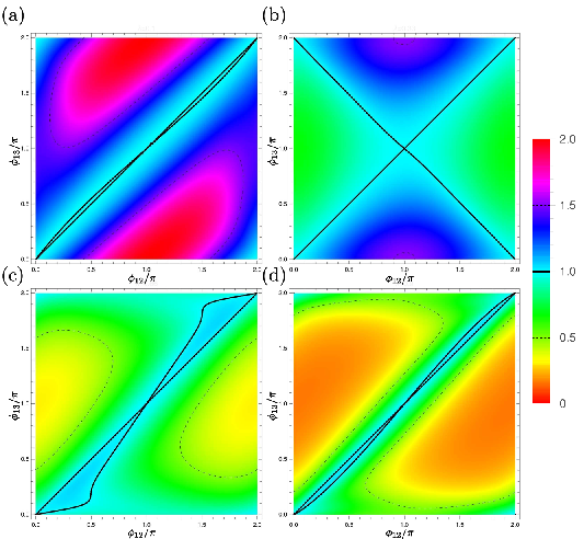
Figure 7: Plot of the ratio (κ1,3​σ1,2N)/(κ1,2​σ1,3N)\left(\kappa_{1,3}\sigma^{N}_{1,2}\right)/\left(\kappa_{1,2}\sigma^{N}_{1,3}\right) for a three terminal non-topological JJ as function of two independent phase differences ϕ12\phi_{12} and ϕ13\phi_{13} for different values of λ\lambda (a) λ=0.1\lambda=0.1 (b) λ=0.33\lambda=0.33 (c) λ=0.66\lambda=0.66 (d) λ=0.9\lambda=0.9. For all the plots we have assumed the temperature to be kB​T=0.5​Δ0k_{B}T=0.5\Delta_{0}. The ratio being equal to 11 is denoted by the solid black lines.

A more detailed figure of the ratio (κ1,3​σ1,2N)/(κ1,2​σ1,3N)\left(\kappa_{1,3}\sigma^{N}_{1,2}\right)/\left(\kappa_{1,2}\sigma^{N}_{1,3}\right) for three terminal non-topological JJ as a function of ϕ12\phi_{12} and ϕ13\phi_{13} for different values of λ\lambda are shown in FIG. 7.

Section G Three terminal normal Josephson junction with pp-wave superconductivity

Refer to caption
Figure 8: Pictorial representation of a three terminal Josephson junction based on normal metal and with pp-wave superconductivity. The coordinate system is chosen in such a way that x=0x=0 at the junction of the three terminals and increases in the direction of superconducting leads.

A Josephson junction based on normal metal with pp-wave superconductivity also hosts Majorana bound states and therefore are topological in nature. We consider the scattering matrix for electrons SeS^{e} at x=0x=0 to be of the same form as in (B48). In this case scattering matrix for hole will be Sh=Se∗S^{h}=S^{e*}. Such junctions can be described using BdG Hamiltonian Thakurathi et al. 2015

ℋ=(−ℏ22​m​∂2∂x2−μ)​τz−i​Δ⁡(x)kF​∂∂x​[cos⁡ϕi​τx−sin⁡ϕi​τy]\mathcal{H}=\left(-\dfrac{\hbar^{2}}{2m}\dfrac{\partial^{2}}{\partial x^{2}}-\mu\right)\uptau_{z}-i\dfrac{\Delta(x)}{k_{F}}\dfrac{\partial}{\partial x}[\cos\phi_{i}\uptau_{x}-\sin\phi_{i}\uptau_{y}] (G99)

where τn\uptau_{n} are the Pauli matrices acting on particle-hole basis; Δ⁡(x)=Δ0​Θ​(x−L)\Delta(x)=\Delta_{0}\Theta(x-L) and ϕi\phi_{i} is the superconducting phase of the iith superconducting lead.

For energies ω<Δ0\omega<\Delta_{0}, the solutions in different regions can be written as

ΨS​i\displaystyle\Psi_{Si} =ai​exp⁡[i​κe′​x]​(ei​θ/2​ei​ϕ(2,3)/2e−iθ/2e−iϕ(2,3)/2)+\displaystyle=a_{i}\exp[i\kappa^{\prime}_{e}x]\begin{pmatrix}e^{i\theta/2}e^{i\phi_{(2,3)}/2}\\ e^{-i\theta/2}e^{-i\phi_{(2,3)}/2}\end{pmatrix}+
bi​exp⁡[−i​κh′​x]​(e−iθ/2ei​ϕ(2,3)/2−ei​θ/2e−iϕ(2,3)/2)\displaystyle~~~~~~~~~~~~~~~b_{i}\exp[-i\kappa^{\prime}_{h}x]\begin{pmatrix}e^{-i\theta/2}e^{i\phi_{(2,3)}/2}\\ -e^{i\theta/2}e^{-i\phi_{(2,3)}/2}\end{pmatrix} (G100)
ΨN​i\displaystyle\Psi_{Ni} =pi​exp⁡[i​ke​x]​(10)+qi​exp⁡[−i​ke​x]​(10)\displaystyle=p_{i}\exp[ik_{e}x]\begin{pmatrix}1\\ 0\end{pmatrix}+q_{i}\exp[-ik_{e}x]\begin{pmatrix}1\\ 0\end{pmatrix}
+ri​exp⁡[i​kh​x]​(01)+si​exp⁡[−i​kh​x]​(01)\displaystyle~~~~~~~~~~~~~~~~+r_{i}\exp[ik_{h}x]\begin{pmatrix}0\\ 1\end{pmatrix}+s_{i}\exp[-ik_{h}x]\begin{pmatrix}0\\ 1\end{pmatrix} (G101)

where θ=arccos⁡(ω/Δ0)\theta=\arccos(\omega/\Delta_0). The subscripts S⁡(N)​iS(N)i denote superconducting (normal) region in the iith (i∈{1,2,3})(i\in\{1,2,3\}) terminal. We consider (due to high doping) κe′≃κh′≃ke≃kh≃kF=(2​m​μ)/ℏ\kappa^{\prime}_{e}\simeq\kappa^{\prime}_{h}\simeq k_{e}\simeq k_{h}\simeq k_{F}=(\sqrt{2m\mu})/\hbar.

By demanding the continuity of the wave functions and their first derivatives across the boundaries and assuming that the amplitudes of the incoming and outgoing waves are related at x=0x=0 by the scattering matrices SeS^{e} and Sh=Se∗S^{h}=S^{e*} we get the condition for bound state

det⁡[𝕀−a2​(ω)​Se​(−ei​ϕ)​Sh​e−i​ϕ]=0\det[\mathbb{I}-a^{2}(\omega)S^{e}(-e^{i\phi})S^{h}e^{-i\phi}]=0 (G102)

where a⁡(ω)=(ωΔ0−i​Δ02−ω2Δ0)a(\omega)=\left(\frac{\omega}{\Delta_{0}}-i\frac{\sqrt{\Delta_{0}^{2}-\omega^{2}}}{\Delta_{0}}\right) and ei​ϕe^{i\phi} is the diagonal matrix with diagonal elements {ei​ϕ1,ei​ϕ2,ei​ϕ3}\{e^{i\phi_{1}},e^{i\phi_{2}},e^{i\phi_{3}}\}.

This gives the bound state energies ω0\omega_{0} and are given by ω=ω00,ω0±\omega=\omega_{0}^{0},\omega_{0}^{\pm} Deb et al. 2018 where

ω00=0\displaystyle\omega_{0}^{0}=0 (G103)
ω0±=±Δ0​τ12​sin2​ϕ122+τ13​sin2​ϕ132+τ23​sin2​ϕ232\displaystyle\omega_{0}^{\pm}=\pm\Delta_{0}\sqrt{\tau_{12}\sin^{2}\frac{\phi_{12}}{2}+\tau_{13}\sin^{2}\frac{\phi_{13}}{2}+\tau_{23}\sin^{2}\frac{\phi_{23}}{2}} (G104)

[ϕi​j=ϕj−ϕi\phi_{ij}=\phi_{j}-\phi_{i}; τi​j=|ti​j|2\tau_{ij}=|t_{ij}|^{2}].

For energies ω>Δ0\omega>\Delta_{0}, we can calculate the total quasiparticle tunnelling probability (𝒯i,j)(\mathcal{T}^{i,j}) from terminal ii to terminal jj. We first consider an electron-like quasiparticle incident on the first superconducting lead. It will give rise to a reflected electron-like and hole-like quasiparticle within the same lead with amplitudes say re​er_{ee} and rh​er_{he} respectively and transmitted electron-like and hole-like quasiparticle in superconducting nnth lead with amplitudes, say, te​en,1t_{ee}^{n,1} and th​en,1t_{he}^{n,1} respectively. The wave functions can be written as

ΨS​1\displaystyle\Psi_{S1} =exp⁡[−i​κe​x]​(eθ/2​ei​ϕ1/2−e−θ/2e−iϕ1/2)+re​e​exp⁡[i​κe​x]​(eθ/2​ei​ϕ1/2e−θ/2e−iϕ1/2)+rh​e​exp⁡[−i​κh​x]​(e−θ/2ei​ϕ1/2−eθ/2e−iϕ1/2)\displaystyle=\exp[-i\kappa_{e}x]\begin{pmatrix}e^{\theta/2}e^{i\phi_{1}/2}\\ -e^{-\theta/2}e^{-i\phi_{1}/2}\end{pmatrix}+r_{ee}\exp[i\kappa_{e}x]\begin{pmatrix}e^{\theta/2}e^{i\phi_{1}/2}\\ e^{-\theta/2}e^{-i\phi_{1}/2}\end{pmatrix}+r_{he}\exp[-i\kappa_{h}x]\begin{pmatrix}e^{-\theta/2}e^{i\phi_{1}/2}\\ -e^{\theta/2}e^{-i\phi_{1}/2}\end{pmatrix} (G105)
ΨS⁡(2,3)\displaystyle\Psi_{S(2,3)} =te​e(2,3),1​exp⁡[i​κe​x]​(eθ/2​ei​ϕ(2,3)/2e−θ/2e−iϕ(2,3)/2)+th​e(2,3),1​exp⁡[−i​κh​x]​(e−θ/2ei​ϕ(2,3)/2−eθ/2e−iϕ(2,3)/2)\displaystyle=t_{ee}^{(2,3),1}\exp[i\kappa_{e}x]\begin{pmatrix}e^{\theta/2}e^{i\phi_{(2,3)}/2}\\ e^{-\theta/2}e^{-i\phi_{(2,3)}/2}\end{pmatrix}+t_{he}^{(2,3),1}\exp[-i\kappa_{h}x]\begin{pmatrix}e^{-\theta/2}e^{i\phi_{(2,3)}/2}\\ -e^{\theta/2}e^{-i\phi_{(2,3)}/2}\end{pmatrix} (G106)
ΨN​i\displaystyle\Psi_{Ni} =pi​exp​[i​ke​x]​(10)+qi​exp​[−i​ke​x]​(10)+ri​exp​[i​kh​x]​(01)+si​exp​[−i​kh​x]​(01)\displaystyle=p_{i}\exp[ik_{e}x]\begin{pmatrix}1\\ 0\end{pmatrix}+q_{i}\exp[-ik_{e}x]\begin{pmatrix}1\\ 0\end{pmatrix}+r_{i}\exp[ik_{h}x]\begin{pmatrix}0\\ 1\end{pmatrix}+s_{i}\exp[-ik_{h}x]\begin{pmatrix}0\\ 1\end{pmatrix} (G107)

where θ=a​r​c​c​o​s​h​(ω/Δ0)\theta=arccosh(\omega/\Delta_{0}). The subscripts S⁡(N)​iS(N)i denote superconducting (normal) region in the iith (i∈{1,2,3})(i\in\{1,2,3\}) terminal. We consider (due to high doping) κe≃κh≃ke≃kh≃kF=(2​m​μ)/ℏ\kappa_{e}\simeq\kappa_{h}\simeq k_{e}\simeq k_{h}\simeq k_{F}=(\sqrt{2m\mu})/\hbar.

By demanding the continuity of the wave functions and their first derivatives across the boundaries and assuming that the amplitudes of the incoming and outgoing waves are related at x=0x=0 by the scattering matrices SeS^{e} and Sh=Se∗S^{h}=S^{e*} we get the values of te​e2,1t_{ee}^{2,1}, th​e2,1t_{he}^{2,1}, te​e3,1t_{ee}^{3,1} and th​e3,1t_{he}^{3,1}. From these, using the relations (C66)-(C74) we calculate

𝒯e2,1=|te​e2,1|2+|th​e2,1|2=τ12​ω2​(ω2−Δ02)​(ω2−|ω0±|2)ω2​(ω2−|ω0±|2)2=τ12​ω2​(ω2−Δ02)​(ω2−|ω0±|2)∏ω0(ω−ω0)2\displaystyle\mathcal{T}_{e}^{2,1}=|t_{ee}^{2,1}|^{2}+|t_{he}^{2,1}|^{2}=\dfrac{\tau_{12}\,\omega^{2}(\omega^{2}-\Delta_{0}^{2})(\omega^{2}-|\omega_{0}^{\pm}|^{2})}{\omega^{2}(\omega^{2}-|\omega_{0}^{\pm}|^{2})^{2}}=\dfrac{\tau_{12}\,\omega^{2}(\omega^{2}-\Delta_{0}^{2})(\omega^{2}-|\omega_{0}^{\pm}|^{2})}{\prod_{\omega_{0}}(\omega-\omega_{0})^{2}} (G108)
𝒯e3,1=|te​e3,1|2+|th​e3,1|2=τ13​ω2​(ω2−Δ02)​(ω2−|ω0±|2)ω2​(ω2−|ω0±|2)2=τ13​ω2​(ω2−Δ02)​(ω2−|ω0±|2)∏ω0(ω−ω0)2\displaystyle\mathcal{T}_{e}^{3,1}=|t_{ee}^{3,1}|^{2}+|t_{he}^{3,1}|^{2}=\dfrac{\tau_{13}\,\omega^{2}(\omega^{2}-\Delta_{0}^{2})(\omega^{2}-|\omega_{0}^{\pm}|^{2})}{\omega^{2}(\omega^{2}-|\omega_{0}^{\pm}|^{2})^{2}}=\dfrac{\tau_{13}\,\omega^{2}(\omega^{2}-\Delta_{0}^{2})(\omega^{2}-|\omega_{0}^{\pm}|^{2})}{\prod_{\omega_{0}}(\omega-\omega_{0})^{2}} (G109)

where ω0±=±Δ0​τ12​sin2​ϕ122+τ13​sin2​ϕ132+τ23​sin2​ϕ232\omega_{0}^{\pm}=\pm\Delta_{0}\sqrt{\tau_{12}\sin^{2}\frac{\phi_{12}}{2}+\tau_{13}\sin^{2}\frac{\phi_{13}}{2}+\tau_{23}\sin^{2}\frac{\phi_{23}}{2}} and (ϕi​j=ϕj−ϕi)(\phi_{ij}=\phi_{j}-\phi_{i}).

Similarly, for a hole-like quasiparticle incident on the first superconducting lead we can calculate te​h2,1t_{eh}^{2,1}, th​h2,1t_{hh}^{2,1}, te​h3,1t_{eh}^{3,1} and th​h3,1t_{hh}^{3,1} and can define

𝒯h2,1\displaystyle\mathcal{T}_{h}^{2,1} =|th​h2,1|2+|te​h2,1|2\displaystyle=|t_{hh}^{2,1}|^{2}+|t_{eh}^{2,1}|^{2} (G110)
𝒯h3,1\displaystyle\mathcal{T}_{h}^{3,1} =|th​h3,1|2+|te​h3,1|2\displaystyle=|t_{hh}^{3,1}|^{2}+|t_{eh}^{3,1}|^{2} (G111)

It turns out that 𝒯h2,1=𝒯e2,1\mathcal{T}_{h}^{2,1}=\mathcal{T}_{e}^{2,1} and 𝒯h3,1=𝒯e3,1\mathcal{T}_{h}^{3,1}=\mathcal{T}_{e}^{3,1} and thus

𝒯2,1\displaystyle\mathcal{T}^{2,1} =𝒯h2,1+𝒯e2,1=2​τ12​(ω2−Δ02)ω2−|ω0±|2\displaystyle=\mathcal{T}_{h}^{2,1}+\mathcal{T}_{e}^{2,1}=2\dfrac{\tau_{12}(\omega^{2}-\Delta_{0}^{2})}{\omega^{2}-|\omega_{0}^{\pm}|^{2}} (G112)
𝒯3,1\displaystyle\mathcal{T}^{3,1} =𝒯h3,1+𝒯e3,1=2​τ13​(ω2−Δ02)ω2−|ω0±|2\displaystyle=\mathcal{T}_{h}^{3,1}+\mathcal{T}_{e}^{3,1}=2\dfrac{\tau_{13}(\omega^{2}-\Delta_{0}^{2})}{\omega^{2}-|\omega_{0}^{\pm}|^{2}} (G113)

With the same spirit we can calculate 𝒯1,2\mathcal{T}^{1,2}, 𝒯3,2\mathcal{T}^{3,2}, 𝒯1,3\mathcal{T}^{1,3} and 𝒯2,3\mathcal{T}^{2,3}. Due to assumed reciprocity of the inter-wire resistance (τi​j=τj​i)(\tau_{ij}=\tau_{ji}), 𝒯i,j=𝒯j,i\mathcal{T}^{i,j}=\mathcal{T}^{j,i}. It can be easily shown that 𝒯i,j\mathcal{T}^{i,j} can be written in general as

𝒯i,j=2​τi​j​ω2​(ω2−Δ02)​(ω2−|ω0±|2)∏ω0(ω−ω0)2=2​τi​j​(ω2−Δ02)ω2−|ω0±|2\mathcal{T}^{i,j}=2\dfrac{\tau_{ij}\,\omega^{2}(\omega^{2}-\Delta_{0}^{2})(\omega^{2}-|\omega_{0}^{\pm}|^{2})}{\prod_{\omega_{0}}(\omega-\omega_{0})^{2}}=2\dfrac{\tau_{ij}(\omega^{2}-\Delta_{0}^{2})}{\omega^{2}-|\omega_{0}^{\pm}|^{2}} (G114)

These expressions are same as that derived in Section D, which readily justifies the fact that the central results of our paper i.e. Eq. (11) and (12) of main text are not only true for a three terminal Josephson junction based on Dirac type spectrum of helical edge states but also for a three terminal Josephson junction made out of 1-D electrons with quadratic dispersion and proximity induced pp-wave superconductivity.

References

  • Maki and Griffin (1965) K. Maki and A. Griffin, Phys. Rev. Lett. 15, 921 (1965).
  • Maki and Griffin (1966) K. Maki and A. Griffin, Phys. Rev. Lett. 16, 258 (1966).
  • Guttman et al. (1997) G. D. Guttman, B. Nathanson, E. Ben-Jacob, and D. J. Bergman, Phys. Rev. B 55, 3849 (1997).
  • Zhao et al. (2003) E. Zhao, T. Löfwander, and J. A. Sauls, Physical review letters 91, 077003 (2003).
  • Zhao et al. (2004) E. Zhao, T. Löfwander, and J. A. Sauls, Physical Review B 69, 134503 (2004).
  • Fornieri et al. (2017) A. Fornieri, G. Timossi, P. Virtanen, P. Solinas, and F. Giazotto, Nature nanotechnology 12, 425 (2017).
  • Luo et al. (2019) X. Luo, Y. Peng, H. Shen, and X. Yi, Scientific reports 9, 2187 (2019).
  • Sothmann and Hankiewicz (2016) B. Sothmann and E. M. Hankiewicz, Physical Review B 94, 081407 (2016).
  • Sothmann et al. (2017) B. Sothmann, F. Giazotto, and E. M. Hankiewicz, New Journal of Physics 19, 023056 (2017).
  • Giazotto and Martínez-Pérez (2012) F. Giazotto and M. J. Martínez-Pérez, Nature 492, 401 (2012).
  • Golubev et al. (2013) D. Golubev, T. Faivre, and J. P. Pekola, Physical Review B 87, 094522 (2013).
  • Martínez-Pérez and Giazotto (2013) M. Martínez-Pérez and F. Giazotto, Applied Physics Letters 102, 182602 (2013).
  • Martínez-Pérez et al. (2014) M. J. Martínez-Pérez, P. Solinas, and F. Giazotto, Journal of Low Temperature Physics 175, 813 (2014).
  • Martínez-Pérez and Giazotto (2014) M. J. Martínez-Pérez and F. Giazotto, Nature communications 5, 3579 (2014).
  • Martínez-Pérez et al. (2015) M. J. Martínez-Pérez, A. Fornieri, and F. Giazotto, Nature nanotechnology 10, 303 (2015).
  • Fornieri et al. (2016a) A. Fornieri, C. Blanc, R. Bosisio, S. D’ambrosio, and F. Giazotto, Nature nanotechnology 11, 258 (2016a).
  • Kolenda et al. (2016) S. Kolenda, M. J. Wolf, and D. Beckmann, Phys. Rev. Lett. 116, 097001 (2016).
  • Fornieri et al. (2016b) A. Fornieri, G. Timossi, R. Bosisio, P. Solinas, and F. Giazotto, Phys. Rev. B 93, 134508 (2016b).
  • Tan et al. (2017) K. Y. Tan, M. Partanen, R. E. Lake, J. Govenius, S. Masuda, and M. Möttönen, Nature communications 8, 15189 (2017).
  • Fornieri and Giazotto (2017) A. Fornieri and F. Giazotto, Nature nanotechnology 12, 944 (2017).
  • Paolucci et al. (2018) F. Paolucci, G. Marchegiani, E. Strambini, and F. Giazotto, Phys. Rev. Applied 10, 024003 (2018).
  • Karimi and Pekola (2018) B. Karimi and J. P. Pekola, Phys. Rev. Applied 10, 054048 (2018).
  • Lutchyn et al. (2010) R. M. Lutchyn, J. D. Sau, and S. Das Sarma, Phys. Rev. Lett. 105, 077001 (2010).
  • Oreg et al. (2010) Y. Oreg, G. Refael, and F. von Oppen, Phys. Rev. Lett. 105, 177002 (2010).
  • Nadj-Perge et al. (2010) S. Nadj-Perge, S. Frolov, E. Bakkers, and L. P. Kouwenhoven, Nature 468, 1084 (2010).
  • Liang and Gao (2012) D. Liang and X. P. Gao, Nano letters 12, 3263 (2012).
  • Mourik et al. (2012) V. Mourik, K. Zuo, S. M. Frolov, S. R. Plissard, E. P. A. M. Bakkers, and L. P. Kouwenhoven, Science 336, 1003 (2012).
  • Das et al. (2012) A. Das, Y. Ronen, Y. Most, Y. Oreg, M. Heiblum, and H. Shtrikman, Nature Physics 8, 887 (2012).
  • Sestoft et al. (2018) J. E. Sestoft, T. Kanne, A. N. Gejl, M. von Soosten, J. S. Yodh, D. Sherman, B. Tarasinski, M. Wimmer, E. Johnson, M. Deng, J. Nygård, T. S. Jespersen, C. M. Marcus, and P. Krogstrup, Phys. Rev. Materials 2, 044202 (2018).
  • Bommer et al. (2019) J. D. S. Bommer, H. Zhang, O. Gül, B. Nijholt, M. Wimmer, F. N. Rybakov, J. Garaud, D. Rodic, E. Babaev, M. Troyer, D. Car, S. R. Plissard, E. P. A. M. Bakkers, K. Watanabe, T. Taniguchi, and L. P. Kouwenhoven, Phys. Rev. Lett. 122, 187702 (2019).
  • König et al. (2007) M. König, S. Wiedmann, C. Brüne, A. Roth, H. Buhmann, L. W. Molenkamp, X.-L. Qi, and S.-C. Zhang, Science 318, 766 (2007).
  • Brüne et al. (2010) C. Brüne, A. Roth, E. G. Novik, M. König, H. Buhmann, E. M. Hankiewicz, W. Hanke, J. Sinova, and L. W. Molenkamp, Nature Physics 6, 448 (2010).
  • Knez et al. (2011) I. Knez, R.-R. Du, and G. Sullivan, Phys. Rev. Lett. 107, 136603 (2011).
  • Brüne et al. (2012) C. Brüne, A. Roth, H. Buhmann, E. M. Hankiewicz, L. W. Molenkamp, J. Maciejko, X.-L. Qi, and S.-C. Zhang, Nature Physics 8, 485 (2012).
  • Knez et al. (2012) I. Knez, R.-R. Du, and G. Sullivan, Phys. Rev. Lett. 109, 186603 (2012).
  • Hart et al. (2014) S. Hart, H. Ren, T. Wagner, P. Leubner, M. Mühlbauer, C. Brüne, H. Buhmann, L. W. Molenkamp, and A. Yacoby, Nature Physics 10, 638 (2014).
  • Kitaev (2001) A. Y. Kitaev, Physics-Uspekhi 44, 131 (2001).
  • Fu and Kane (2009) L. Fu and C. L. Kane, Physical Review B 79, 161408 (2009).
  • Nilsson et al. (2008) J. Nilsson, A. R. Akhmerov, and C. W. J. Beenakker, Phys. Rev. Lett. 101, 120403 (2008).
  • (40) Topological JJ refers to those JJ where the sub-gap bound state formed at the junction are primarily due to overlap of Majorana bound state appearing at the ends of the topological supercondcutors.
  • Laroche et al. (2019) D. Laroche, D. Bouman, D. J. van Woerkom, A. Proutski, C. Murthy, D. I. Pikulin, C. Nayak, R. J. van Gulik, J. Nygård, P. Krogstrup, et al., Nature communications 10, 245 (2019).
  • Bocquillon et al. (2017) E. Bocquillon, R. S. Deacon, J. Wiedenmann, P. Leubner, T. M. Klapwijk, C. Brüne, K. Ishibashi, H. Buhmann, and L. W. Molenkamp, Nature nanotechnology 12, 137 (2017).
  • Kwon et al. (2004) H.-J. Kwon, K. Sengupta, and V. M. Yakovenko, The European Physical Journal B - Condensed Matter and Complex Systems 37, 349 (2004).
  • Pershoguba and Glazman (2019) S. S. Pershoguba and L. I. Glazman, Phys. Rev. B 99, 134514 (2019).
  • Guttman et al. (1998) G. D. Guttman, E. Ben-Jacob, and D. J. Bergman, Phys. Rev. B 57, 2717 (1998).
  • Sauls (2018) J. A. Sauls, “Andreev bound states and their signatures,” (2018).
  • Beenakker (1991) C. W. J. Beenakker, Phys. Rev. Lett. 67, 3836 (1991).
  • Octavio et al. (1983) M. Octavio, M. Tinkham, G. E. Blonder, and T. M. Klapwijk, Phys. Rev. B 27, 6739 (1983).
  • Bardeen et al. (1969) J. Bardeen, R. Kümmel, A. E. Jacobs, and L. Tewordt, Phys. Rev. 187, 556 (1969).
  • (50) This is so because each topological superconductor will contribute a single Majorana to the Josephson tri-junction but two of them will hybridize and gap out while the third MBS will stay topologically protected.
  • De Gennes (2018) P.-G. De Gennes, Superconductivity of metals and alloys (CRC Press, 2018).
  • Deb et al. (2018) O. Deb, K. Sengupta, and D. Sen, Physical Review B 97, 174518 (2018).
  • Dolcini et al. (2015) F. Dolcini, M. Houzet, and J. S. Meyer, Physical Review B 92, 035428 (2015).
  • Fu and Kane (2008) L. Fu and C. L. Kane, Physical review letters 100, 096407 (2008).
  • Landauer (1957a) R. Landauer, IBM J. Res. Dev. 1, 223 (1957a).
  • Moskalets (2011) M. Moskalets, Scattering Matrix Approach to Non-Stationary Quantum Transport: Chapter 1 (2011) pp. 1–33.
  • (57) If a​r​g⁡(S)i,j≠a​r​g⁡(S)j,i\mathop{arg}\nolimits{(S)_{i,j}}\not=\mathop{arg}\nolimits{(S)_{j,i}} then the relative phase of the scattering matrix leads to a additive contribution to ϕi,j\phi_{i,j} leading to anomalous Josepson current.
  • Alicea (2012) J. Alicea, Reports on progress in physics 75, 076501 (2012).
  • Houzet and Meyer (2019) M. Houzet and J. S. Meyer, Physical Review B 100, 014521 (2019).
  • Bauer and Sothmann (2019) A. G. Bauer and B. Sothmann, Physical Review B 99, 214508 (2019).
  • Landauer (1957b) R. Landauer, IBM Journal of Research and Development 1, 223 (1957b).
  • Beenakker (1992) C. Beenakker, Physical Review B 46, 12841 (1992).
  • Wadhawan et al. (2018) D. Wadhawan, K. Roychowdhury, P. Mehta, and S. Das, Phys. Rev. B 98, 155113 (2018).
  • Calzona and Trauzettel (2019) A. Calzona and B. Trauzettel, arXiv preprint arXiv:1909.06280 (2019).
  • (65) FIG. 2 of main text.
  • (66) FIG. 2 of main text.
  • Brouwer and Beenakker (1997) P. Brouwer and C. Beenakker, Chaos, Solitons & Fractals 8, 1249 (1997).
  • Thakurathi et al. (2015) M. Thakurathi, O. Deb, and D. Sen, Journal of Physics: Condensed Matter 27, 275702 (2015).