跳到论文正文
W Papers独立论文阅读器 arXiv:1912.12804 论文正文 计算阅读时间 · 0%
引用这篇论文根据当前论文元数据生成,正式投稿前建议核对。


License: arXiv.org perpetual non-exclusive license
arXiv:1912.12804v2 [cs.IT] 09 Mar 2020

Joint Sparse Recovery Using Signal Space Matching Pursuit

*Junhan Kim    Jian Wang    *Luong Trung Nguyen       *Byonghyo Shim    Department of Electrical    Computer Engineering    Seoul National University    Seoul    Korea School of Data Science    Fudan University    Shanghai    China Email: {junhankim    ltnguyen    bshim}@islab.snu.ac.kr    jian_wang@fudan.edu.cn Thanks: This work was supported in part by the MSIT (Ministry of Science and ICT), Korea, under the ITRC (Information Technology Research Center) support program (IITP-2020-2017-0-01637) supervised by the IITP (Institute for Information & communications Technology Promotion) and in part by the Samsung Research Funding & Incubation Center for Future Technology of Samsung Electronics under Grant SRFC-IT1901-17. Thanks: This paper was presented in part at the IEEE International Symposium on Information Theory, Colorado, USA, June, 2018˜[1]. (Junhan Kim and Jian Wang equally contributed to this work.)(Corresponding author: Byonghyo Shim.)
Abstract

In this paper, we put forth a new joint sparse recovery algorithm called signal space matching pursuit (SSMP). The key idea of the proposed SSMP algorithm is to sequentially investigate the support of jointly sparse vectors to minimize the subspace distance to the residual space. Our performance guarantee analysis indicates that SSMP accurately reconstructs any row KK-sparse matrix of rank rr in the full row rank scenario if the sampling matrix 𝐀\mathbf{A} satisfies krank(𝐀)≥K+1\operatornamewithlimits{krank}(\mathbf{A})\geq K+1, which meets the fundamental minimum requirement on 𝐀\mathbf{A} to ensure exact recovery. We also show that SSMP guarantees exact reconstruction in at most K−r+⌈rL⌉K-r+\lceil\frac{r}{L}\rceil iterations, provided that 𝐀\mathbf{A} satisfies the restricted isometry property (RIP) of order L⁡(K−r)+r+1L(K-r)+r+1 with

δL⁡(K−r)+r+1<max⁡{rK+r4+r4,LK+1.15​L},\delta_{L(K-r)+r+1}<\max\left\{\frac{\sqrt{r}}{\sqrt{K+\frac{r}{4}}+\sqrt{\frac{r}{4}}},\frac{\sqrt{L}}{\sqrt{K}+1.15\sqrt{L}}\right\},

where LL is the number of indices chosen in each iteration. This implies that the requirement on the RIP constant becomes less restrictive when rr increases. Such behavior seems to be natural but has not been reported for most of conventional methods. We also show that if r=1r=1, then by running more than KK iterations, the performance guarantee of SSMP can be improved to δ⌊7.8​K⌋≤0.155\delta_{\lfloor 7.8K\rfloor}\leq 0.155. Furthermore, we show that under a suitable RIP condition, the reconstruction error of SSMP is upper bounded by a constant multiple of the noise power, which demonstrates the robustness of SSMP to measurement noise. Finally, from extensive numerical experiments, we show that SSMP outperforms conventional joint sparse recovery algorithms both in noiseless and noisy scenarios.

Index Terms:
Joint sparse recovery, multiple measurement vectors (MMV), subspace distance, rank aware order recursive matching pursuit (RA-ORMP), orthogonal least squares (OLS), restricted isometry property (RIP)

I Introduction

In recent years, sparse signal recovery has received considerable attention in image processing, seismology, data compression, source localization, wireless communication, machine learning, to name just a few [3, 2, 4, 5]. The main goal of sparse signal recovery is to reconstruct a high dimensional KK-sparse vector 𝐱∈ℝn\mathbf{x}\in\mathbb{R}^{n} (‖𝐱‖0≤K≪n\|\mathbf{x}\|_{0}\leq K\ll n where ‖𝐱‖0\|\mathbf{x}\|_{0} denotes the number of nonzero elements in 𝐱\mathbf{x}) from its compressed linear measurements

𝐲=𝐀𝐱,\mathbf{y}=\mathbf{A}\mathbf{x}, (1)

where 𝐀∈ℝm×n\mathbf{A}\in\mathbb{R}^{m\times n} (m≪nm\ll n) is the sampling (sensing) matrix. In various applications, such as wireless channel estimation [6, 5], sub-Nyquist sampling of multiband signals [7, 8], angles of departure and arrival (AoD and AoA) estimation in mmWave communication systems [9], and brain imaging [10], we encounter a situation where multiple measurement vectors (MMV) of a group of jointly sparse vectors are available. By the jointly sparse vectors, we mean multiple sparse vectors having a common support (the index set of nonzero entries). In this situation, one can dramatically improve reconstruction accuracy by recovering all the desired sparse vectors simultaneously [11, 12]. The problem to reconstruct a group {𝐱i}i=1r\{\mathbf{x}_{i}\}_{i=1}^{r} of jointly KK-sparse vectors11 1 In the sequel, we assume that 𝐱1,…,𝐱r\mathbf{x}_{1},{\color[rgb]{0,0,1}{\ldots}},\mathbf{x}_{r} are linearly independent. is often referred to as the joint sparse recovery problem [17]. Let 𝐲i=𝐀𝐱i\mathbf{y}_{i}=\mathbf{A}\mathbf{x}_{i} be the measurement vector of 𝐱i\mathbf{x}_{i} acquired through the sampling matrix 𝐀\mathbf{A}. Then the system model describing the MMV can be expressed as

𝐘=𝐀𝐗,\mathbf{Y}=\mathbf{A}\mathbf{X}, (2)

where 𝐘=[𝐲1,…,𝐲r]\mathbf{Y}=[\mathbf{y}_{1},\ldots,\mathbf{y}_{r}] and 𝐗=[𝐱1,…,𝐱r]\mathbf{X}=[\mathbf{x}_{1},\ldots,\mathbf{x}_{r}].

The main task of joint sparse recovery problems is to identify the common support shared by the unknown sparse signals. Once the support is determined accurately, then the system model in (2) can be reduced to rr independent overdetermined systems and thus the solutions can be found via the conventional least squares (LS) approach. The problem to identify the support can be formulated as

minS⊂{1,…,n}|S|s.t.𝐲1,…,𝐲r∈ℛ⁡(𝐀S),\begin{split}&\underset{S\subset\{1,\ldots,n\}}{\min}\penalty\ \penalty\ \penalty\ \penalty\ |S|\\ &\penalty\ \penalty\ \penalty\ \penalty\ \text{s.t.}\penalty\ \penalty\ \penalty\ \penalty\ \penalty\ \penalty\ \penalty\ \mathbf{y}_{1},\ldots,\mathbf{y}_{r}\in\mathcal{R}(\mathbf{A}_{S}),\end{split} (3)

where 𝐀S\mathbf{A}_{S} is the submatrix of 𝐀\mathbf{A} that contains the columns indexed by SS and ℛ⁡(𝐀S)\mathcal{R}(\mathbf{A}_{S}) is the subspace spanned by the columns of 𝐀S\mathbf{A}_{S}. A naive way to solve (3) is to search over all possible subspaces spanned by 𝐀\mathbf{A}. Such a combinatorial search, however, is exhaustive and thus infeasible for most practical scenarios. Over the years, various approaches to address this problem have been proposed [11, 12, 13, 14, 15, 17, 16]. Roughly speaking, these approaches can be classified into two categories: 1) those based on greedy search principles (e.g., simultaneous orthogonal matching pursuit (SOMP) [13] and rank aware order recursive matching pursuit (RA-ORMP) [16]) and 2) those relying on convex optimization (e.g., mixed norm minimization [14]). Hybrid approaches combining greedy search techniques and conventional methods such as multiple signal classification (MUSIC) have also been proposed (e.g., compressive MUSIC (CS-MUSIC) [15] and subspace-augmented MUSIC (SA-MUSIC) [17]).

In this paper, we put forth a new algorithm, called signal space matching pursuit (SSMP), to improve the quality of joint sparse recovery. Basically, the SSMP algorithm identifies columns of 𝐀\mathbf{A} that span the measurement space. By the measurement space, we mean the subspace ℛ⁡(𝐘)\mathcal{R}(\mathbf{Y}) spanned by the measurement vectors 𝐲1,…,𝐲r\mathbf{y}_{1},\ldots,\mathbf{y}_{r}. Towards this end, we recast (3) as

minS⊂{1,…,n}|S|s.t.ℛ⁡(𝐘)⊆ℛ⁡(𝐀S).\begin{split}&\underset{S\subset\{1,\ldots,n\}}{\min}\penalty\ \penalty\ \penalty\ \penalty\ |S|\\ &\penalty\ \penalty\ \penalty\ \penalty\ \text{s.t.}\penalty\ \penalty\ \penalty\ \penalty\ \penalty\ \penalty\ \penalty\ \mathcal{R}(\mathbf{Y})\subseteq\mathcal{R}(\mathbf{A}_{S}).\end{split} (4)

In solving this problem, SSMP exploits the notion of subspace distance which measures the closeness between two vector spaces (see Definition 1 in Section II-A) [18]. Specifically, SSMP chooses multiple, say LL, columns of 𝐀\mathbf{A} that minimize the subspace distance to the measurement space in each iteration.

The contributions of this paper are as follows:

  • 1)

    We propose a new joint sparse recovery algorithm called SSMP (Section II). From the simulation results, we show that SSMP outperforms conventional techniques both in noiseless and noisy scenarios (Section VI). Specifically, in the noiseless scenario, the critical sparsity (the maximum sparsity level at which exact reconstruction is ensured [22]) of SSMP is about 1.5 times higher than those obtained by conventional techniques. In the noisy scenario, SSMP performs close to the oracle least squares (Oracle-LS) estimator22 2 Oracle-LS is the estimator that provides the best achievable bound using prior knowledge on the common support. in terms of the mean square error (MSE) when the signal-to-noise ratio (SNR) is high.

  • 2)

    We analyze a condition under which the SSMP algorithm exactly reconstructs any group of jointly KK-sparse vectors in at most KK iterations in the noiseless scenario (Section III).

    • –

      In the full row rank scenario (r=Kr=K),33 3 Note that 𝐗\mathbf{X} has at most KK nonzero rows so that r=rank(𝐗)≤Kr=\operatornamewithlimits{rank}(\mathbf{X})\leq K. In this sense, we refer to the case where r=Kr=K as the full row rank scenario. we show that SSMP accurately recovers any group {𝐱i}i=1r\{\mathbf{x}_{i}\}_{i=1}^{r} of jointly KK-sparse vectors in ⌈KL⌉\lceil\frac{K}{L}\rceil iterations if the sampling matrix 𝐀\mathbf{A} satisfies (Theorem 1(i))

      krank(𝐀)\displaystyle\operatornamewithlimits{krank}(\mathbf{A}) ≥K+1,\displaystyle\geq K+1,

      where krank(𝐀)\operatornamewithlimits{krank}(\mathbf{A}) is the maximum number of columns in 𝐀\mathbf{A} that are linearly independent. This implies that under a mild condition on 𝐀\mathbf{A} (any mm columns of 𝐀\mathbf{A} are linearly independent), SSMP guarantees exact reconstruction with m=K+1m=K+1 measurements, which meets the fundamental minimum requirement on the number of measurements to ensure perfect recovery of {𝐱i}i=1r\{\mathbf{x}_{i}\}_{i=1}^{r} [16].

    • –

      In the rank deficient scenario (r<Kr<K), we show that SSMP reconstructs {𝐱i}i=1r\{\mathbf{x}_{i}\}_{i=1}^{r} accurately in at most K−r+⌈rL⌉K-r+\lceil\frac{r}{L}\rceil iterations if 𝐀\mathbf{A} satisfies the restricted isometry property (RIP [27]) of order L⁡(K−r)+r+1L(K-r)+r+1 with (Theorem 1(ii))

      δL⁡(K−r)+r+1\displaystyle\delta_{L(K-r)+r+1} <max⁡{rK+r4+r4,LK+1.15​L}.\displaystyle<\max\left\{\frac{\sqrt{r}}{\sqrt{K+\frac{r}{4}}+\sqrt{\frac{r}{4}}},\frac{\sqrt{L}}{\sqrt{K}+1.15\sqrt{L}}\right\}. (5)

      Using the monotonicity of the RIP constant (see Lemma 3), one can notice that the requirement on the RIP constant becomes less restrictive when the number rr of (linearly independent) measurement vectors increases. This behavior seems to be natural but has not been reported for conventional methods such as SOMP [13] and mixed norm minimization [14]. In particular, if rr is on the order of KK, e.g., r=⌈K2⌉r=\lceil\frac{K}{2}\rceil, then (5) is satisfied under

      δL⁡(K−⌈K2⌉)+⌈K2⌉+1<12,\delta_{L(K-\lceil\frac{K}{2}\rceil)+\lceil\frac{K}{2}\rceil+1}<\frac{1}{2},

      which implies that SSMP ensures exact recovery with overwhelming probability as long as the number of random measurements scales linearly with K​log⁡nKK\log\frac{n}{K} [27, 31].

  • 3)

    We analyze the performance of SSMP in the scenario where the observation matrix 𝐘\mathbf{Y} is contaminated by noise (Section IV). Specifically, we show that under a suitable RIP condition, the reconstruction error of SSMP is upper bounded by a constant multiple of the noise power (Theorems 2 and 3), which demonstrates the robustness of SSMP to measurement noise.

  • 4)

    As a special case, when r=1r=1, we establish the performance guarantee of SSMP running more than KK iterations (Section V). Specifically, we show that SSMP exactly recovers any KK-sparse vector in max⁡{K,⌊8​KL⌋}\max\{K,\lfloor\frac{8K}{L}\rfloor\} iterations under (Theorem 5)

    δ⌊7.8​K⌋≤0.155.\delta_{\lfloor 7.8K\rfloor}\leq 0.155.

    In contrast to (5), this bound is a constant and unrelated to the sparsity KK. This implies that even when rr is not on the order of KK, SSMP guarantees exact reconstruction with 𝒪⁡(K​log⁡nK)\mathcal{O}(K\log\frac{n}{K}) random measurements by running slightly more than KK iterations.

We briefly summarize the notations used in this paper.

  • •

    Let Ω={1,…,n}\Omega=\{1,{\color[rgb]{0,0,1}{\ldots}},n\};

  • •

    For J⊂ΩJ\subset\Omega, |J||J| is the cardinality of JJ and Ω∖J\Omega\setminus J is the set of all indices in Ω\Omega but not in JJ;

  • •

    For a vector 𝐱\mathbf{x}, 𝐱J∈ℝ|J|\mathbf{x}_{J}\in\mathbb{R}^{|J|} is the restriction of 𝐱\mathbf{x} to the elements indexed by JJ;

  • •

    We refer to 𝐗\mathbf{X} having at most KK nonzero rows as a row KK-sparse signal and define its support SS as the index set of its nonzero rows;44 4 For example, if 𝐱1=[1 0 0 2]′\mathbf{x}_{1}=[1\ 0\ 0\ 2]^{\prime} and 𝐱2=[2 0 0 1]′\mathbf{x}_{2}=[2\ 0\ 0\ 1]^{\prime}, then 𝐗=[𝐱1​𝐱2]\mathbf{X}=[\mathbf{x}_{1}\ \mathbf{x}_{2}] is a row 22-sparse matrix with support {1,4}\{1,4\}.

  • •

    The submatrix of 𝐗\mathbf{X} containing the rows indexed by JJ is denoted by 𝐗J\mathbf{X}^{J};

We use the following notations for a general matrix 𝐇∈ℝm×n\mathbf{H}\in\mathbb{R}^{m\times n}.

  • •

    The ii-th column of 𝐇\mathbf{H} is denoted by 𝐡i∈ℝm\mathbf{h}_{i}\in\mathbb{R}^{m};

  • •

    The jj-th row of 𝐇\mathbf{H} is denoted by 𝐡j∈ℝn\mathbf{h}^{j}\in\mathbb{R}^{n};

  • •

    The submatrix of 𝐇\mathbf{H} containing the columns indexed by JJ is denoted by 𝐇J\mathbf{H}_{J};

  • •

    If 𝐇J\mathbf{H}_{J} has full column rank, 𝐇J†=(𝐇J′​𝐇J)−1​𝐇J′\mathbf{H}_{J}^{\dagger}=(\mathbf{H}_{J}^{\prime}\mathbf{H}_{J})^{-1}\mathbf{H}_{J}^{\prime} is the pseudoinverse of 𝐇J\mathbf{H}_{J} where 𝐇J′\mathbf{H}_{J}^{\prime} is the transpose of 𝐇J\mathbf{H}_{J};

  • •

    We define ℛ⁡(𝐇)\mathcal{R}(\mathbf{H}) as the column space of 𝐇\mathbf{H};

  • •

    The Frobenius norm and the spectral norm of 𝐇\mathbf{H} are denoted by ‖𝐇‖F\|\mathbf{H}\|_{F} and ‖𝐇‖2\|\mathbf{H}\|_{2}, respectively;

  • •

    The mixed ℓ1,2\ell_{1,2}-norm of 𝐇\mathbf{H} is denoted by ‖𝐇‖1,2\|\mathbf{H}\|_{1,2}, i.e., ‖𝐇‖1,2=∑j=1m‖𝐡j‖2\|\mathbf{H}\|_{1,2}=\sum_{j=1}^{m}\|\mathbf{h}^{j}\|_{2};

  • •

    The minimum, maximum, and ii-th largest singular values of 𝐇\mathbf{H} are denoted by σmin​(𝐇)\sigma_{\min}(\mathbf{H}), σmax​(𝐇)\sigma_{\max}(\mathbf{H}), and σi​(𝐇)\sigma_{i}(\mathbf{H}), respectively;

  • •

    The orthogonal projections onto a subspace 𝒱⊂ℝm\mathcal{V}\subset\mathbb{R}^{m} and its orthogonal complement 𝒱⟂\mathcal{V}^{\perp} are denoted by 𝐏𝒱\mathbf{P}_{\mathcal{V}} and 𝐏𝒱⟂\mathbf{P}_{\mathcal{V}}^{\perp}, respectively. For simplicity, we write 𝐏J\mathbf{P}_{J} and 𝐏J⟂\mathbf{P}_{J}^{\perp} instead of 𝐏ℛ⁡(𝐀J)\mathbf{P}_{\mathcal{R}(\mathbf{A}_{J})} and 𝐏ℛ⁡(𝐀J)⟂\mathbf{P}_{\mathcal{R}(\mathbf{A}_{J})}^{\perp}, respectively.

II The Proposed SSMP Algorithm

As mentioned, we use the notion of subspace distance in solving our main problem (4). In this section, we briefly introduce the definition of subspace distance and its properties, and then describe the proposed SSMP algorithm.

II-A Preliminaries

We begin with the definition of subspace distance. In a nutshell, the subspace distance is minimized if two subspaces coincide with each other and maximized if two subspaces are perpendicular to each other.

Definition 1 (Subspace distance [18]).

Let 𝒱\mathcal{V} and 𝒲\mathcal{W} be subspaces in ℝm\mathbb{R}^{m}, and let {𝐯1,…,𝐯p}\{\mathbf{v}_{1},\ldots,\mathbf{v}_{p}\} and {𝐰1,…,𝐰q}\{\mathbf{w}_{1},\ldots,\mathbf{w}_{q}\} be orthonormal bases of 𝒱\mathcal{V} and 𝒲\mathcal{W}, respectively. Then the subspace distance dist(𝒱,𝒲)\operatornamewithlimits{dist}(\mathcal{V},\mathcal{W}) between 𝒱\mathcal{V} and 𝒲\mathcal{W} is

dist(𝒱,𝒲)\displaystyle\operatornamewithlimits{dist}(\mathcal{V},\mathcal{W}) =max⁡{p,q}−∑i=1𝑝​∑j=1𝑞​|⟨𝐯i,𝐰j⟩|2.\displaystyle=\sqrt{\max\{p,q\}-\underset{i=1}{\overset{p}{\sum}}\underset{j=1}{\overset{q}{\sum}}|\langle\mathbf{v}_{i},\mathbf{w}_{j}\rangle|^{2}}. (6)

Refer to caption

Figure 1: Subspace distance between one-dimensional subspaces.

As a special case, suppose 𝒱\mathcal{V} and 𝒲\mathcal{W} are one-dimensional subspaces in ℝm\mathbb{R}^{m} (i.e., 𝒱\mathcal{V} and 𝒲\mathcal{W} are two lines in ℝm\mathbb{R}^{m}). Further, let {𝐯}\{\mathbf{v}\} and {𝐰}\{\mathbf{w}\} be orthonormal bases of 𝒱\mathcal{V} and 𝒲\mathcal{W}, respectively, and θ\theta be the angle between 𝐯\mathbf{v} and 𝐰\mathbf{w}. Then the subspace distance dist(𝒱,𝒲)\operatornamewithlimits{dist}(\mathcal{V},\mathcal{W}) between 𝒱\mathcal{V} and 𝒲\mathcal{W} is (see Fig. 1)

dist(𝒱,𝒲)\displaystyle\operatornamewithlimits{dist}(\mathcal{V},\mathcal{W}) =(a)​1−|⟨𝐯,𝐰⟩|2\displaystyle\overset{(a)}{=}\sqrt{1-|\langle\mathbf{v},\mathbf{w}\rangle|^{2}}
=1−(‖𝐯‖2​‖𝐰‖2​cos⁡θ)2\displaystyle=\sqrt{1-(\|\mathbf{v}\|_{2}\|\mathbf{w}\|_{2}\cos\theta)^{2}}
=sin⁡θ,\displaystyle=\sin\theta, (7)

where (a) is because 𝒱\mathcal{V} and 𝒲\mathcal{W} are one-dimensional (i.e., p=q=1p=q=1 in (6)). One can easily see that dist(𝒱,𝒲)\operatornamewithlimits{dist}(\mathcal{V},\mathcal{W}) is maximal when θ=π2\theta=\frac{\pi}{2} (i.e., 𝒱⟂𝒲\mathcal{V}\perp\mathcal{W}) and dist(𝒱,𝒲)=0\operatornamewithlimits{dist}(\mathcal{V},\mathcal{W})=0 if and only if θ=0\theta=0 (i.e., 𝒱=𝒲\mathcal{V}=\mathcal{W}). In fact, dist(𝒱,𝒲)\operatornamewithlimits{dist}(\mathcal{V},\mathcal{W}) is maximized when 𝒱\mathcal{V} and 𝒲\mathcal{W} are orthogonal and dist(𝒱,𝒲)=0\operatornamewithlimits{dist}(\mathcal{V},\mathcal{W})=0 if and only if 𝒱\mathcal{V} and 𝒲\mathcal{W} coincide with each other [18]. Also, note that the subspace distance is a proper metric between subspaces since it satisfies the following three properties of a metric [18, 19]:

  • (i)

    dist(𝒱,𝒲)≥0\operatornamewithlimits{dist}(\mathcal{V},\mathcal{W})\geq 0 for any subspaces 𝒱,𝒲⊂ℝm\mathcal{V},\mathcal{W}\subset\mathbb{R}^{m}, and the equality holds if and only if 𝒱=𝒲\mathcal{V}=\mathcal{W}.

  • (ii)

    dist(𝒱,𝒲)=dist(𝒲,𝒱)\operatornamewithlimits{dist}(\mathcal{V},\mathcal{W})=\operatornamewithlimits{dist}(\mathcal{W},\mathcal{V}) for any subspaces 𝒱,𝒲⊂ℝm\mathcal{V},\mathcal{W}\subset\mathbb{R}^{m}.

  • (iii)

    dist(𝒰,𝒲)≤dist(𝒰,𝒱)+dist(𝒱,𝒲)\operatornamewithlimits{dist}(\mathcal{U},\mathcal{W})\leq\operatornamewithlimits{dist}(\mathcal{U},\mathcal{V})+\operatornamewithlimits{dist}(\mathcal{V},\mathcal{W}) for any subspaces 𝒰,𝒱,𝒲⊂ℝm\mathcal{U},\mathcal{V},\mathcal{W}\subset\mathbb{R}^{m}.

Exploiting the subspace distance, (4) can be reformulated as

minS⊂Ω|S|s.t.dist(ℛ⁡(𝐘),𝐏S​ℛ​(𝐘))=0,\begin{split}&\underset{S\subset\Omega}{\min}\penalty\ \penalty\ \penalty\ |S|\\ &\penalty\ \text{s.t.}\penalty\ \penalty\ \penalty\ \operatornamewithlimits{dist}\left(\mathcal{R}(\mathbf{Y}),\mathbf{P}_{S}\mathcal{R}(\mathbf{Y})\right)=0,\end{split} (8)

where 𝐏S​ℛ​(𝐘)={𝐏S​𝐳:𝐳∈ℛ⁡(𝐘)}\mathbf{P}_{S}\mathcal{R}(\mathbf{Y})=\{\mathbf{P}_{S}\mathbf{z}:\mathbf{z}\in\mathcal{R}(\mathbf{Y})\}.

Lemma 1.

Problems (4) and (8) are equivalent.

Proof.

It suffices to show that two constraints ℛ⁡(𝐘)⊆ℛ⁡(𝐀S)\mathcal{R}(\mathbf{Y})\subseteq\mathcal{R}(\mathbf{A}_{S}) and dist(ℛ⁡(𝐘),𝐏S​ℛ​(𝐘))=0\operatornamewithlimits{dist}\left(\mathcal{R}(\mathbf{Y}),\mathbf{P}_{S}\mathcal{R}(\mathbf{Y})\right)=0 are equivalent. If dist(ℛ⁡(𝐘),𝐏S​ℛ​(𝐘))=0\operatornamewithlimits{dist}\left(\mathcal{R}(\mathbf{Y}),\mathbf{P}_{S}\mathcal{R}(\mathbf{Y})\right)=0, then ℛ⁡(𝐘)=𝐏S​ℛ​(𝐘)⊆ℛ⁡(𝐀S)\mathcal{R}(\mathbf{Y})=\mathbf{P}_{S}\mathcal{R}(\mathbf{Y})\subseteq\mathcal{R}(\mathbf{A}_{S}) by the property (i) of the subspace distance. Conversely, if ℛ⁡(𝐘)⊆ℛ⁡(𝐀S)\mathcal{R}(\mathbf{Y})\subseteq\mathcal{R}(\mathbf{A}_{S}), then 𝐏S​ℛ​(𝐘)=ℛ⁡(𝐘)\mathbf{P}_{S}\mathcal{R}(\mathbf{Y})=\mathcal{R}(\mathbf{Y}) and thus dist(ℛ⁡(𝐘),𝐏S​ℛ​(𝐘))=0\operatornamewithlimits{dist}\left(\mathcal{R}(\mathbf{Y}),\mathbf{P}_{S}\mathcal{R}(\mathbf{Y})\right)=0. ∎

It is worth mentioning that problem (8) can be extended to the noisy scenario by relaxing the constraint dist(ℛ⁡(𝐘),𝐏S​(ℛ⁡(𝐘)))=0\operatornamewithlimits{dist}\left(\mathcal{R}(\mathbf{Y}),\mathbf{P}_{S}\left(\mathcal{R}(\mathbf{Y})\right)\right)=0 to dist(ℛ⁡(𝐘),𝐏S​(ℛ⁡(𝐘)))≤ϵ\operatornamewithlimits{dist}\left(\mathcal{R}(\mathbf{Y}),\mathbf{P}_{S}\left(\mathcal{R}(\mathbf{Y})\right)\right)\leq\epsilon for some properly chosen threshold ϵ>0\epsilon>0.

II-B Algorithm Description

The proposed SSMP algorithm solves problem (8) using the greedy principle. Note that the greedy principle has been popularly used in sparse signal recovery for its computational simplicity and competitive performance [20, 21, 22, 23]. In a nutshell, SSMP sequentially investigates the support to minimize the subspace distance to the residual space.

In the first iteration, SSMP chooses multiple, say LL, columns of the sampling matrix 𝐀\mathbf{A} that minimize the subspace distance to the measurement space ℛ⁡(𝐘)\mathcal{R}(\mathbf{Y}). Towards this end, SSMP computes the subspace distance

di=dist(ℛ⁡(𝐘),𝐏{i}​ℛ​(𝐘))d_{i}=\operatornamewithlimits{dist}\left(\mathcal{R}(\mathbf{Y}),\mathbf{P}_{\{i\}}\mathcal{R}(\mathbf{Y})\right)

between ℛ⁡(𝐘)\mathcal{R}(\mathbf{Y}) and its orthogonal projection 𝐏{i}​ℛ​(𝐘)\mathbf{P}_{\{i\}}\mathcal{R}(\mathbf{Y}) onto the subspace spanned by each column 𝐚i\mathbf{a}_{i} of 𝐀\mathbf{A}. Let 0≤di1≤di2≤…≤din0\leq d_{i_{1}}\leq d_{i_{2}}\leq\ldots\leq d_{i_{n}}, then SSMP chooses i1,…,iLi_{1},\ldots,i_{L} (the indices corresponding to the LL smallest subspace distances). In other words, the estimated support S1={i1,…,iL}S^{1}=\{i_{1},\ldots,i_{L}\} is given by

S1\displaystyle S^{1} =arg⁡minI:I⊂Ω,|I|=L∑i∈Idi\displaystyle=\underset{I:I\subset\Omega,|I|=L}{\arg\min}\sum_{i\in I}d_{i}
=arg⁡minI:I⊂Ω,|I|=L∑i∈Idist(ℛ(𝐘),𝐏{i}ℛ(𝐘)).\displaystyle=\underset{I:I\subset\Omega,|I|=L}{\arg\min}\sum_{i\in I}\operatornamewithlimits{dist}\left(\mathcal{R}(\mathbf{Y}),\mathbf{P}_{\{i\}}\mathcal{R}(\mathbf{Y})\right). (9)

For example, let 𝐲∈ℝ2\mathbf{y}\in\mathbb{R}^{2}, 𝐀∈ℝ2×3\mathbf{A}\in\mathbb{R}^{2\times 3}, and θi\theta_{i} be the angle between ℛ⁡(𝐲)\mathcal{R}(\mathbf{y}) and 𝐏{i}​ℛ​(𝐲)\mathbf{P}_{\{i\}}\mathcal{R}(\mathbf{y}) (see Fig. 2). Also, suppose SSMP picks up two indices in each iteration (i.e., L=2L=2). Then, by (7), di=dist(ℛ⁡(𝐲),𝐏{i}​ℛ​(𝐲))=sin⁡θid_{i}=\operatornamewithlimits{dist}\left(\mathcal{R}(\mathbf{y}),\mathbf{P}_{\{i\}}\mathcal{R}(\mathbf{y})\right)=\sin\theta_{i} so that d2<d3<d1d_{2}<d_{3}<d_{1} (see θ2<θ3<θ1\theta_{2}<\theta_{3}<\theta_{1} in Fig. 2) and S1={2,3}S^{1}=\{2,3\}. After updating the support set S1S^{1}, SSMP computes the estimate 𝐗1\mathbf{X}^{1} of the desired signal 𝐗\mathbf{X} by solving the LS problem:

𝐗1\displaystyle\mathbf{X}^{1} =arg⁡min𝐔:supp(𝐔)⊂S1∥𝐘−𝐀𝐔∥F.\displaystyle=\underset{\mathbf{U}:\operatornamewithlimits{supp}(\mathbf{U})\subset S^{1}}{\arg\min}\|\mathbf{Y}-\mathbf{A}\mathbf{U}\|_{F}.

Note that (𝐗1)S1=𝐀S1†​𝐘(\mathbf{X}^{1})^{S^{1}}=\mathbf{A}_{S^{1}}^{\dagger}\mathbf{Y} and (𝐗1)Ω∖S1=𝟎|Ω∖S1|×r(\mathbf{X}^{1})^{\Omega\setminus S^{1}}=\mathbf{0}_{|\Omega\setminus S^{1}|\times r}, where 𝟎d1×d2\mathbf{0}_{d_{1}\times d_{2}} is the (d1×d2)(d_{1}\times d_{2})-dimensional zero matrix. Finally, SSMP generates the residual matrix

𝐑1=𝐘−𝐀𝐗1=𝐘−𝐀S1​(𝐗1)S1=𝐘−𝐀S1​𝐀S1†​𝐘=𝐏S1⟂​𝐘,\mathbf{R}^{1}=\mathbf{Y}-\mathbf{A}\mathbf{X}^{1}=\mathbf{Y}-\mathbf{A}_{S^{1}}(\mathbf{X}^{1})^{S^{1}}=\mathbf{Y}-\mathbf{A}_{S^{1}}\mathbf{A}_{S^{1}}^{\dagger}\mathbf{Y}=\mathbf{P}_{S^{1}}^{\perp}\mathbf{Y},

which will be used as an observation matrix for the next iteration.
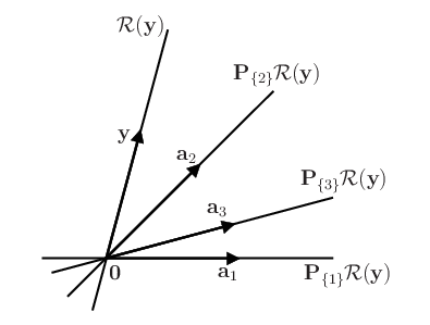
Refer to caption

Figure 2: Illustration of the identification step of the SSMP algorithm. In the first iteration, SSMP (L=2)(L=2) chooses S1={2,3}S^{1}=\{2,3\}.

The general iteration of SSMP is similar to the first iteration except for the fact that the residual space is used instead of the measurement space ℛ⁡(𝐘)\mathcal{R}(\mathbf{Y}) in the support identification. In other words, SSMP identifies the columns of 𝐀\mathbf{A} that minimize the subspace distance to the residual space ℛ⁡(𝐑k−1)\mathcal{R}(\mathbf{R}^{k-1}) in the kk-th iteration. Let IkI^{k} be the set of LL indices newly chosen in the kk-th iteration, then

Ik\displaystyle I^{k} =arg⁡minI:I⊂Ω∖Sk−1,|I|=L∑i∈Idist(ℛ(𝐑k−1),𝐏Sk−1∪{i}ℛ(𝐑k−1)).\displaystyle=\underset{I:I\subset\Omega\setminus S^{k-1},|I|=L}{\arg\min}\sum_{i\in I}\operatornamewithlimits{dist}\left(\mathcal{R}(\mathbf{R}^{k-1}),\mathbf{P}_{S^{k-1}\cup\{i\}}\mathcal{R}(\mathbf{R}^{k-1})\right). (10)

These set of operations are repeated until the iteration number reaches the maximum value kmax=min⁡{K,⌊mL⌋}k_{\max}=\min\{K,\lfloor\frac{m}{L}\rfloor\}55 5 In the estimation step, SSMP computes (𝐗k)Sk=𝐀Sk†​𝐘=(𝐀Sk′​𝐀Sk)−1​𝐀Sk′​𝐘(\mathbf{X}^{k})^{S^{k}}=\mathbf{A}_{S^{k}}^{\dagger}\mathbf{Y}=(\mathbf{A}_{S^{k}}^{\prime}\mathbf{A}_{S^{k}})^{-1}\mathbf{A}_{S^{k}}^{\prime}\mathbf{Y}. In order to perform this task, 𝐀Sk\mathbf{A}_{S^{k}} should have full column rank and thus |Sk|=k​L≤m|S^{k}|=kL\leq m. or the pre-defined stopping criterion

dist(ℛ⁡(𝐘),𝐏Sk​ℛ​(𝐘))≤ϵ\operatornamewithlimits{dist}(\mathcal{R}(\mathbf{Y}),\mathbf{P}_{S^{k}}\mathcal{R}(\mathbf{Y}))\leq\epsilon

is satisfied (ϵ\epsilon is a stopping threshold).

Suppose SSMP runs kk iterations in total and more than KK indices are chosen (i.e., |Sk|>K|S^{k}|>K). Then, by identifying the KK rows of 𝐗k\mathbf{X}^{k} with largest ℓ2\ell_{2}-norms, the estimated support SkS^{k} is pruned to its subset S^\widehat{S} consisting of KK elements, i.e.,

S^\displaystyle\widehat{S} =arg⁡minJ:|J|=K∥𝐗k−(𝐗k)J∥F.\displaystyle=\underset{J:|J|=K}{\arg\min}\penalty\ \|\mathbf{X}^{k}-(\mathbf{X}^{k})^{J}\|_{F}.

Finally, SSMP computes the row KK-sparse estimate 𝐗^\widehat{\mathbf{X}} of 𝐗\mathbf{X} by solving the LS problem on S^\widehat{S}. This pruning step, also known as debiasing, helps to reduce the reconstruction error ‖𝐗−𝐗^‖F\|\mathbf{X}-\widehat{\mathbf{X}}\|_{F} in the noisy scenario [34].

II-C Refined Identification Rule

As shown in (10), in the kk-th iteration, SSMP computes the subspace distance between the residual space ℛ⁡(𝐑k−1)\mathcal{R}(\mathbf{R}^{k-1}) and its projection space 𝐏Sk−1∪{i}​ℛ​(𝐑k−1)\mathbf{P}_{S^{k-1}\cup\{i\}}\mathcal{R}(\mathbf{R}^{k-1}) for all remaining indices ii. Since this operation requires n−(k−1)​Ln-(k-1)L projection operators 𝐏Sk−1∪{i}\mathbf{P}_{S^{k-1}\cup\{i\}}, it would clearly be computationally prohibitive, especially for large nn. In view of this, it is of importance to come up with a computationally efficient way to perform the support identification. In the following proposition, we introduce a simplified selection rule under which the number of projections required in each identification step is independent of the signal dimension nn.

Proposition 1.

Consider the system model in (2). Suppose the SSMP algorithm chooses LL indices in each iteration. Then the set Ik+1I^{k+1} of LL indices chosen in the (k+1)(k+1)-th iteration satisfies

Ik+1\displaystyle I^{k+1} =arg⁡maxI:I⊂Ω∖Sk,|I|=L∑i∈I‖𝐏ℛ⁡(𝐑k)𝐏Sk⟂​𝐚i‖𝐏Sk⟂​𝐚i‖2‖2.\displaystyle=\underset{I:I\subset\Omega\setminus S^{k},|I|=L}{\arg\max}\penalty\ \underset{i\in I}{\sum}\left\|\mathbf{P}_{\mathcal{R}(\mathbf{R}^{k})}\frac{\mathbf{P}_{S^{k}}^{\perp}\mathbf{a}_{i}}{\|\mathbf{P}_{S^{k}}^{\perp}\mathbf{a}_{i}\|_{2}}\right\|_{2}. (11)
Proof.

See Appendix A. ∎

Note that the selection rule in (11) requires only two projection operators 𝐏ℛ⁡(𝐑k)\mathbf{P}_{\mathcal{R}(\mathbf{R}^{k})} and 𝐏Sk⟂\mathbf{P}_{S^{k}}^{\perp} in each identification step. One can also observe from (11) that SSMP performs the identification step by one simple matrix multiplication followed by the selection of LL columns with largest ℓ2\ell_{2}-norms. Specifically, if 𝐁∈ℝm×n\mathbf{B}\in\mathbb{R}^{m\times n} is the ℓ2\ell_{2}-normalized counterpart of 𝐏Sk⟂​𝐀\mathbf{P}_{S^{k}}^{\perp}\mathbf{A}, i.e.,

𝐛i={𝐏Sk⟂​𝐚i‖𝐏Sk⟂​𝐚i‖2,i∈Ω∖Sk,𝟎m×1,i∈Sk,\mathbf{b}_{i}=\begin{cases}\frac{\mathbf{P}_{S^{k}}^{\perp}\mathbf{a}_{i}}{\|\mathbf{P}_{S^{k}}^{\perp}\mathbf{a}_{i}\|_{2}},&i\in\Omega\setminus S^{k},\\ \mathbf{0}_{m\times 1},&i\in S^{k},\end{cases}

then SSMP picks LL column indices of 𝐏ℛ⁡(𝐑k)​𝐁\mathbf{P}_{\mathcal{R}(\mathbf{R}^{k})}\mathbf{B} with largest ℓ2\ell_{2}-norms. In Algorithm 1, we summarize the proposed SSMP algorithm.

Algorithm 1 The SSMP algorithm
0:  sampling matrix 𝐀∈ℝm×n\mathbf{A}\in\mathbb{R}^{m\times n}, observation matrix 𝐘∈ℝm×r\mathbf{Y}\in\mathbb{R}^{m\times r}, sparsity KK, number LL of selected indices per iteration, and stopping threshold ϵ\epsilon.
0:  iteration counter k=0k=0, estimated support S0=∅S^{0}=\emptyset, and residual matrix 𝐑0=𝐘\mathbf{R}^{0}=\mathbf{Y}.
1:  While k<min⁡{K,⌊mL⌋}k<\min\{K,\lfloor\frac{m}{L}\rfloor\} and dist(ℛ⁡(𝐘),𝐏Sk​ℛ​(𝐘))>ϵ\operatornamewithlimits{dist}(\mathcal{R}(\mathbf{Y}),\mathbf{P}_{S^{k}}\mathcal{R}(\mathbf{Y}))>\epsilon do
2:  k=k+1k=k+1;
3:  Construct the ℓ2\ell_{2}-normalized counterpart 𝐁\mathbf{B} of 𝐏Sk−1⟂​𝐀\mathbf{P}_{S^{k-1}}^{\perp}\mathbf{A}, i.e., 𝐛i=𝐏Sk−1⟂​𝐚i/‖𝐏Sk−1⟂​𝐚i‖2\mathbf{b}_{i}=\mathbf{P}_{S^{k-1}}^{\perp}\mathbf{a}_{i}/\|\mathbf{P}_{S^{k-1}}^{\perp}\mathbf{a}_{i}\|_{2} for each of i∈Ω∖Sk−1i\in\Omega\setminus S^{k-1} and 𝐛i=𝟎m×1\mathbf{b}_{i}=\mathbf{0}_{m\times 1} for each of i∈Sk−1i\in S^{k-1};
4:  Identify the indices ϕ⁡(1),…,ϕ⁡(L)\phi(1),\ldots,\phi(L) of LL columns in 𝐏ℛ⁡(𝐑k−1)​𝐁\mathbf{P}_{\mathcal{R}(\mathbf{R}^{k-1})}\mathbf{B} with largest ℓ2\ell_{2}-norms;
5:  Sk=Sk−1∪{ϕ⁡(1),…,ϕ⁡(L)}S^{k}=S^{k-1}\cup\{\phi(1),\ldots,\phi(L)\};
6:  𝐗k=arg⁡min𝐔:supp(𝐔)⊂Sk∥𝐘−𝐀𝐔∥F\mathbf{X}^{k}=\underset{\mathbf{U}:\operatornamewithlimits{supp}(\mathbf{U})\subset S^{k}}{\arg\min}\|\mathbf{Y}-\mathbf{A}\mathbf{U}\|_{F};
7:  𝐑k=𝐘−𝐀𝐗k\mathbf{R}^{k}=\mathbf{Y}-\mathbf{A}\mathbf{X}^{k};
8:  end while
8:  S^=arg⁡minJ:|J|=K∥𝐗k−(𝐗k)J∥F\widehat{S}=\underset{J:|J|=K}{\arg\min}\|\mathbf{X}^{k}-(\mathbf{X}^{k})^{J}\|_{F} and 𝐗^\widehat{\mathbf{X}} satisfying 𝐗^S^=𝐀S^†​𝐘\widehat{\mathbf{X}}^{\widehat{S}}=\mathbf{A}_{\widehat{S}}^{\dagger}\mathbf{Y} and 𝐗^Ω∖S^=𝟎|Ω∖S^|×r\widehat{\mathbf{X}}^{\Omega\setminus\widehat{S}}=\mathbf{0}_{|\Omega\setminus\widehat{S}|\times r}.

III Exact Joint Sparse Recovery via SSMP

In this section, we analyze a sufficient condition under which SSMP recovers any row KK-sparse matrix accurately in the noiseless scenario. In this case, we set the stopping threshold ϵ\epsilon to zero. Also, we assume that the number LL of indices chosen in each iteration satisfies L≤min⁡{K,mK}L\leq\min\{K,\frac{m}{K}\}. Then SSMP performs at most KK iterations before stopping (see Algorithm 1). Finally, we assume that the sampling matrix 𝐀\mathbf{A} has unit ℓ2\ell_{2}-norm columns since the performance of SSMP is not affected by the ℓ2\ell_{2}-normalization of columns in 𝐀\mathbf{A}.66 6 Note that the term 𝐏Sk⟂​𝐚i/‖𝐏Sk⟂​𝐚i‖2\mathbf{P}_{S^{k}}^{\perp}\mathbf{a}_{i}/\|\mathbf{P}_{S^{k}}^{\perp}\mathbf{a}_{i}\|_{2} in (11) is not affected by the ℓ2\ell_{2}-normalization of columns in 𝐀\mathbf{A}.

III-A Definition and Lemmas

In our analysis, we employ the RIP framework, a widely used tool to analyze sparse recovery algorithms [25, 21, 22, 26, 23, 24].

Definition 2 (RIP [27]).

A matrix 𝐀∈ℝm×n\mathbf{A}\in\mathbb{R}^{m\times n} is said to satisfy the RIP of order KK if there exists a constant δ∈(0,1)\delta\in(0,1) such that

(1−δ)​‖𝐱‖22≤‖𝐀𝐱‖22≤(1+δ)​‖𝐱‖22\displaystyle(1-\delta)\|\mathbf{x}\|_{2}^{2}\leq\|\mathbf{A}\mathbf{x}\|_{2}^{2}\leq(1+\delta)\|\mathbf{x}\|_{2}^{2} (12)

for any KK-sparse vector 𝐱∈ℝn\mathbf{x}\in\mathbb{R}^{n}. In particular, the minimum value of δ\delta satisfying (12) is called the RIP constant and denoted by δK\delta_{K}.

We next introduce several lemmas useful in our analysis.

Lemma 2 ([17, Lemma A.2]).

Let 𝐀∈ℝm×n\mathbf{A}\in\mathbb{R}^{m\times n} and S,J⊂ΩS,J\subset\Omega with S∖J≠∅S\setminus J\neq\emptyset, then

σmin​(𝐏J⟂​𝐀S∖J)≥σmin​(𝐀S∪J).\sigma_{\min}(\mathbf{P}_{J}^{\perp}\mathbf{A}_{S\setminus J})\geq\sigma_{\min}(\mathbf{A}_{S\cup J}).

Lemma 2 implies that if 𝐀S∪J\mathbf{A}_{S\cup J} has full column rank, so does the projected matrix 𝐏J⟂​𝐀S∖J\mathbf{P}_{J}^{\perp}\mathbf{A}_{S\setminus J}. The next lemma describes the monotonicity of the RIP constant.

Lemma 3 ([22, Lemma 1]).

If a matrix 𝐀\mathbf{A} satisfies the RIP of orders K1K_{1} and K2K_{2} (K1≤K2)(K_{1}\leq K_{2}), then δK1≤δK2\delta_{K_{1}}\leq\delta_{K_{2}}.

Lemma 4 ([28, Lemma 1]).

Let 𝐀∈ℝm×n\mathbf{A}\in\mathbb{R}^{m\times n} and S,J⊂ΩS,J\subset\Omega. If 𝐀\mathbf{A} satisfies the RIP of order |S∪J||S\cup J|, then for any 𝐳∈ℝ|S∖J|\mathbf{z}\in\mathbb{R}^{|S\setminus J|},

(1−δ|S∪J|)​‖𝐳‖22≤‖𝐏J⟂​𝐀S∖J​𝐳‖22≤(1+δ|S∪J|)​‖𝐳‖22.\displaystyle(1-\delta_{|S\cup J|})\|\mathbf{z}\|_{2}^{2}\leq\|\mathbf{P}_{J}^{\perp}\mathbf{A}_{S\setminus J}\mathbf{z}\|_{2}^{2}\leq(1+\delta_{|S\cup J|})\|\mathbf{z}\|_{2}^{2}.

Lemma 4 implies that if 𝐀\mathbf{A} satisfies the RIP of order |S∪J||S\cup J|, then the projected matrix 𝐏J⟂​𝐀S∖J\mathbf{P}_{J}^{\perp}\mathbf{A}_{S\setminus J} obeys the RIP of order |S∖J||S\setminus J| and the corresponding RIP constant δ|S∖J|​(𝐏J⟂​𝐀S∖J)\delta_{|S\setminus J|}(\mathbf{P}_{J}^{\perp}\mathbf{A}_{S\setminus J}) satisfies δ|S∖J|​(𝐏J⟂​𝐀S∖J)≤δ|S∪J|\delta_{|S\setminus J|}(\mathbf{P}_{J}^{\perp}\mathbf{A}_{S\setminus J})\leq\delta_{|S\cup J|}.

Recall that the SSMP algorithm picks the indices of the LL largest elements in {‖𝐏ℛ⁡(𝐑k)​𝐛i‖2:i∈Ω∖Sk}\{\|\mathbf{P}_{\mathcal{R}(\mathbf{R}^{k})}\mathbf{b}_{i}\|_{2}:i\in\Omega\setminus S^{k}\} in the (k+1)(k+1)-th iteration, where 𝐁\mathbf{B} is the ℓ2\ell_{2}-normalized counterpart of 𝐏Sk⟂​𝐀\mathbf{P}_{S^{k}}^{\perp}\mathbf{A} (see Algorithm 1). This implies that SSMP chooses at least one support element in the (k+1)(k+1)-th iteration if and only if the largest element in {‖𝐏ℛ⁡(𝐑k)​𝐛i‖2:i∈S∖Sk}\{\|\mathbf{P}_{\mathcal{R}(\mathbf{R}^{k})}\mathbf{b}_{i}\|_{2}:i\in S\setminus S^{k}\} is larger than the LL-th largest element in {‖𝐏ℛ⁡(𝐑k)​𝐛i‖2:i∈Ω∖(S∪Sk)}\{\|\mathbf{P}_{\mathcal{R}(\mathbf{R}^{k})}\mathbf{b}_{i}\|_{2}:i\in\Omega\setminus(S\cup S^{k})\}. The following lemma provides a lower bound of maxi∈S∖Sk⁡‖𝐏ℛ⁡(𝐑k)​𝐛i‖2\max_{i\in S\setminus S^{k}}\|\mathbf{P}_{\mathcal{R}(\mathbf{R}^{k})}\mathbf{b}_{i}\|_{2}.

Lemma 5.

Consider the system model in (2). Let SkS^{k} be the estimated support and 𝐑k\mathbf{R}^{k} be the residual generated in the k-th iteration of the SSMP algorithm. Also, let 𝐁\mathbf{B} be the ℓ2\ell_{2}-normalized counterpart of 𝐏Sk⟂​𝐀\mathbf{P}_{S^{k}}^{\perp}\mathbf{A}. If 𝐀S∪Sk\mathbf{A}_{S\cup S^{k}} has full column rank and |S∖Sk|>0|S\setminus S^{k}|>0, then

maxi∈S∖Sk⁡‖𝐏ℛ⁡(𝐑k)​𝐛i‖22\displaystyle\max_{i\in S\setminus S^{k}}\|\mathbf{P}_{\mathcal{R}(\mathbf{R}^{k})}\mathbf{b}_{i}\|_{2}^{2} ≥1|S∖Sk|​∑i∈S∖Sk‖𝐏ℛ⁡(𝐑k)​𝐛i‖22\displaystyle\geq\frac{1}{|S\setminus S^{k}|}\sum_{i\in S\setminus S^{k}}\|\mathbf{P}_{\mathcal{R}(\mathbf{R}^{k})}\mathbf{b}_{i}\|_{2}^{2}
≥1|S∖Sk|​∑i=1dσ|S∖Sk|+1−i2​(𝐁S∖Sk),\displaystyle\geq\frac{1}{|S\setminus S^{k}|}\sum_{i=1}^{d}\sigma_{|S\setminus S^{k}|+1-i}^{2}(\mathbf{B}_{S\setminus S^{k}}), (13)

where d=rank(𝐗S∖Sk)d=\operatornamewithlimits{rank}(\mathbf{X}^{S\setminus S^{k}}).

Proof.

See Appendix C. ∎

The following lemmas play an important role in bounding the LL-th largest element in {‖𝐏ℛ⁡(𝐑k)​𝐛i‖2:i∈Ω∖(S∪Sk)}\{\|\mathbf{P}_{\mathcal{R}(\mathbf{R}^{k})}\mathbf{b}_{i}\|_{2}:i\in\Omega\setminus(S\cup S^{k})\}.

Lemma 6 ([29, Lemma 3]).

Let 𝐀∈ℝm×n\mathbf{A}\in\mathbb{R}^{m\times n} and S,J⊂ΩS,J\subset\Omega. If 𝐀\mathbf{A} satisfies the RIP of order |S∪J|+1|S\cup J|+1, then for any i∈Ω∖(S∪J)i\in\Omega\setminus(S\cup J),

‖𝐏ℛ⁡(𝐏J⟂​𝐀S∖J)⟂​𝐏J⟂​𝐚i‖22\displaystyle\|\mathbf{P}_{\mathcal{R}(\mathbf{P}_{J}^{\perp}\mathbf{A}_{S\setminus J})}^{\perp}\mathbf{P}_{J}^{\perp}\mathbf{a}_{i}\|_{2}^{2} ≥(1−δ|S∪J|+12)​‖𝐏J⟂​𝐚i‖22.\displaystyle\geq(1-\delta_{|S\cup J|+1}^{2})\|\mathbf{P}_{J}^{\perp}\mathbf{a}_{i}\|_{2}^{2}.
Lemma 7 ([28, Lemma 2]).

Let 𝐀∈ℝm×n\mathbf{A}\in\mathbb{R}^{m\times n} and S,J,Λ⊂ΩS,J,\Lambda\subset\Omega with (S∪J)∩Λ=∅(S\cup J)\cap\Lambda=\emptyset. If 𝐀\mathbf{A} satisfies the RIP of order |S∪J|+|Λ||S\cup J|+|\Lambda|, then for any 𝐳∈ℝ|S∖J|\mathbf{z}\in\mathbb{R}^{|S\setminus J|},

‖𝐀Λ′​𝐏J⟂​𝐀S∖J​𝐳‖2≤δ|S∪J|+|Λ|​‖𝐳‖2.\|\mathbf{A}_{\Lambda}^{\prime}\mathbf{P}_{J}^{\perp}\mathbf{A}_{S\setminus J}\mathbf{z}\|_{2}\leq\delta_{|S\cup J|+|\Lambda|}\|\mathbf{z}\|_{2}.

III-B Performance Guarantee of SSMP

We now analyze a condition of SSMP to guarantee exact reconstruction of any row KK-sparse signal in KK iterations. In the sequel, we say that SSMP is successful in the kk-th iteration if at least one support element is chosen (i.e., Ik∩S≠∅I^{k}\cap S\neq\emptyset). First, we present a condition under which SSMP chooses at least K−rK-r support elements in the first K−rK-r iterations (i.e., |S∩SK−r|≥K−r|S\cap S^{K-r}|\geq K-r).

Proposition 2.

Consider the system model in (2), where 𝐀\mathbf{A} has unit ℓ2\ell_{2}-norm columns and any rr nonzero rows of 𝐗\mathbf{X} are linearly independent. Let LL be the number of indices chosen in each iteration of the SSMP algorithm. If 𝐀\mathbf{A} satisfies the RIP of order L⁡(K−r)+r+1L(K-r)+r+1 with

δL⁡(K−r)+r+1\displaystyle\delta_{L(K-r)+r+1} <max⁡{rK+r4+r4,LK+1.15​L},\displaystyle<\max\left\{\frac{\sqrt{r}}{\sqrt{K+\frac{r}{4}}+\sqrt{\frac{r}{4}}},\frac{\sqrt{L}}{\sqrt{K}+1.15\sqrt{L}}\right\}, (14)

then SSMP picks at least K−rK-r support elements in the first K−rK-r iterations.

Proof.

We show that |S∩Sk|≥k|S\cap S^{k}|\geq k for each of k∈{0,…,K−r}k\in\{0,\ldots,K-r\}. First, we consider the case where k=0k=0. This case is trivial since S0=∅S^{0}=\emptyset and thus

|S∩S0|=0.|S\cap S^{0}|=0.

Next, we assume that |S∩Sk|≥k|S\cap S^{k}|\geq k for some integer k⁡(0≤k<K−r)k\penalty\ (0\leq k<K-r). In other words, we assume that the SSMP algorithm chooses at least kk support elements in the first kk iterations. In particular, we consider the case where |S∩Sk|=k|S\cap S^{k}|=k, since otherwise |S∩Sk+1|≥|S∩Sk|≥k+1|S\cap S^{k+1}|\geq|S\cap S^{k}|\geq k+1. Under this assumption, we show that SSMP picks at least one support element in the (k+1)(k+1)-th iteration. As mentioned, SSMP is successful in the (k+1)(k+1)-th iteration if and only if the largest element p1p_{1} in {‖𝐏ℛ⁡(𝐑k)​𝐛i‖2}i∈S∖Sk\{\|\mathbf{P}_{\mathcal{R}(\mathbf{R}^{k})}\mathbf{b}_{i}\|_{2}\}_{i\in S\setminus S^{k}} is larger than the LL-th largest element qLq_{L} in {‖𝐏ℛ⁡(𝐑k)​𝐛i‖2}i∈Ω∖(S∪Sk)\{\|\mathbf{P}_{\mathcal{R}(\mathbf{R}^{k})}\mathbf{b}_{i}\|_{2}\}_{i\in\Omega\setminus(S\cup S^{k})}. In our proof, we build a lower bound of p1p_{1} and an upper bound of qLq_{L} and then show that the former is larger than the latter under (14).

∙\bullet Lower bound of p1p_{1}:

Note that |S∖Sk|=|S|−|S∩Sk|=K−k>r|S\setminus S^{k}|=|S|-|S\cap S^{k}|=K-k>r. Then, rank(𝐗S∖Sk)≥r\operatornamewithlimits{rank}(\mathbf{X}^{S\setminus S^{k}})\geq r since any rr nonzero rows of 𝐗\mathbf{X} are linearly independent. Also, note that rank(𝐗S∖Sk)≤r\operatornamewithlimits{rank}(\mathbf{X}^{S\setminus S^{k}})\leq r since 𝐗S∖Sk\mathbf{X}^{S\setminus S^{k}} consists of rr columns. As a result, we have

rank(𝐗S∖Sk)\displaystyle\operatornamewithlimits{rank}(\mathbf{X}^{S\setminus S^{k}}) =r.\displaystyle=r. (15)

In addition, since

|S∪Sk|\displaystyle|S\cup S^{k}| =|Sk|+|S∖Sk|=L​k+K−k\displaystyle=|S^{k}|+|S\setminus S^{k}|=Lk+K-k
≤(L−1)​(K−r−1)+K=L⁡(K−r−1)+r+1,\displaystyle\leq(L-1)(K-r-1)+K=L(K-r-1)+r+1, (16)

𝐀\mathbf{A} satisfies the RIP of order |S∪Sk||S\cup S^{k}|. Then, by Lemma 5, we have

p12\displaystyle p_{1}^{2} =maxi∈S∖Sk⁡‖𝐏ℛ⁡(𝐑k)​𝐛i‖22≥r​σmin2​(𝐁S∖Sk)K−k.\displaystyle=\max_{i\in S\setminus S^{k}}\|\mathbf{P}_{\mathcal{R}(\mathbf{R}^{k})}\mathbf{b}_{i}\|_{2}^{2}\geq\frac{r\sigma_{\min}^{2}(\mathbf{B}_{S\setminus S^{k}})}{K-k}. (17)

Let 𝐃=diag​{‖𝐏Sk⟂​𝐚i‖2:i∈S∖Sk}\mathbf{D}=\text{diag}\{\|\mathbf{P}_{S^{k}}^{\perp}\mathbf{a}_{i}\|_{2}:i\in S\setminus S^{k}\}, then

σmin2​(𝐁S∖Sk)\displaystyle\sigma_{\min}^{2}(\mathbf{B}_{S\setminus S^{k}}) =σmin2​(𝐏Sk⟂​𝐀S∖Sk​𝐃−1)\displaystyle\hskip 1.05273pt=\sigma_{\min}^{2}(\mathbf{P}_{S^{k}}^{\perp}\mathbf{A}_{S\setminus S^{k}}\mathbf{D}^{-1})
≥σmin2​(𝐏Sk⟂​𝐀S∖Sk)​σmin2​(𝐃−1)\displaystyle\hskip 1.05273pt\geq\sigma_{\min}^{2}(\mathbf{P}_{S^{k}}^{\perp}\mathbf{A}_{S\setminus S^{k}})\sigma_{\min}^{2}(\mathbf{D}^{-1})
=σmin2​(𝐏Sk⟂​𝐀S∖Sk)maxi∈S∖Sk⁡‖𝐏Sk⟂​𝐚i‖22\displaystyle\hskip 1.05273pt=\frac{\sigma_{\min}^{2}(\mathbf{P}_{S^{k}}^{\perp}\mathbf{A}_{S\setminus S^{k}})}{\max_{i\in S\setminus S^{k}}\|\mathbf{P}_{S^{k}}^{\perp}\mathbf{a}_{i}\|_{2}^{2}}
≥(a)​σmin2​(𝐏Sk⟂​𝐀S∖Sk),\displaystyle\overset{(a)}{\geq}\sigma_{\min}^{2}(\mathbf{P}_{S^{k}}^{\perp}\mathbf{A}_{S\setminus S^{k}}), (18)

where (a) is because ‖𝐏Sk⟂​𝐚i‖22≤‖𝐚i‖22=1\|\mathbf{P}_{S^{k}}^{\perp}\mathbf{a}_{i}\|_{2}^{2}\leq\|\mathbf{a}_{i}\|_{2}^{2}=1 for each of i∈S∖Ski\in S\setminus S^{k}. Note that 𝐀\mathbf{A} satisfies the RIP of order |S∪Sk||S\cup S^{k}|. Then, by Lemma 4, the projected matrix 𝐏Sk⟂​𝐀S∖Sk\mathbf{P}_{S^{k}}^{\perp}\mathbf{A}_{S\setminus S^{k}} obeys the RIP of order |S∖Sk||S\setminus S^{k}| and the corresponding RIP constant δ|S∖Sk|​(𝐏Sk⟂​𝐀S∖Sk)\delta_{|S\setminus S^{k}|}(\mathbf{P}_{S^{k}}^{\perp}\mathbf{A}_{S\setminus S^{k}}) satisfies

δ|S∖Sk|​(𝐏Sk⟂​𝐀S∖Sk)\displaystyle\delta_{|S\setminus S^{k}|}(\mathbf{P}_{S^{k}}^{\perp}\mathbf{A}_{S\setminus S^{k}}) ≤δ|S∪Sk|.\displaystyle\leq\delta_{|S\cup S^{k}|}. (19)

Also, by the definition of the RIP (see Definition 2), we have

σmin2​(𝐏Sk⟂​𝐀S∖Sk)\displaystyle\sigma_{\min}^{2}(\mathbf{P}_{S^{k}}^{\perp}\mathbf{A}_{S\setminus S^{k}}) ≥1−δ|S∖Sk|​(𝐏Sk⟂​𝐀S∖Sk).\displaystyle\geq 1-\delta_{|S\setminus S^{k}|}(\mathbf{P}_{S^{k}}^{\perp}\mathbf{A}_{S\setminus S^{k}}). (20)

Finally, by combining (17)-(20), we obtain

p12\displaystyle p_{1}^{2} ≥r⁡(1−δ|S∪Sk|)K−k≥r⁡(1−δL⁡(K−r)+r+1)K,\displaystyle\geq\frac{r(1-\delta_{|S\cup S^{k}|})}{K-k}\geq\frac{r(1-\delta_{L(K-r)+r+1})}{K}, (21)

where the last inequality follows from Lemma 3.

∙\bullet Upper bound of qLq_{L}:

We build an upper bound of qLq_{L} in two different ways and combine the results.

First, let ψl\psi_{l} be the index corresponding to the ll-th largest element qlq_{l} in {‖𝐏ℛ⁡(𝐑k)​𝐛i‖2}i∈Ω∖(S∪Sk)\left\{\left\|\mathbf{P}_{\mathcal{R}(\mathbf{R}^{k})}\mathbf{b}_{i}\right\|_{2}\right\}_{i\in\Omega\setminus(S\cup S^{k})} and Λ={ψ1,…,ψL}\Lambda=\{\psi_{1},\ldots,\psi_{L}\}. Since ℛ⁡(𝐑k)=ℛ⁡(𝐏Sk⟂​𝐀S∖Sk​𝐗S∖Sk)⊆ℛ⁡(𝐏Sk⟂​𝐀S∖Sk)\mathcal{R}(\mathbf{R}^{k})=\mathcal{R}(\mathbf{P}_{S^{k}}^{\perp}\mathbf{A}_{S\setminus S^{k}}\mathbf{X}^{S\setminus S^{k}})\subseteq\mathcal{R}(\mathbf{P}_{S^{k}}^{\perp}\mathbf{A}_{S\setminus S^{k}}), we have

qL2\displaystyle q_{L}^{2} =‖𝐏ℛ⁡(𝐑k)​𝐏Sk⟂​𝐚ψL‖𝐏Sk⟂​𝐚ψL‖2‖22\displaystyle=\left\|\mathbf{P}_{\mathcal{R}(\mathbf{R}^{k})}\frac{\mathbf{P}_{S^{k}}^{\perp}\mathbf{a}_{\psi_{L}}}{\|\mathbf{P}_{S^{k}}^{\perp}\mathbf{a}_{\psi_{L}}\|_{2}}\right\|_{2}^{2}
≤‖𝐏ℛ⁡(𝐏Sk⟂​𝐀S∖Sk)​𝐏Sk⟂​𝐚ψL‖𝐏Sk⟂​𝐚ψL‖2‖22\displaystyle\leq\left\|\mathbf{P}_{\mathcal{R}(\mathbf{P}_{S^{k}}^{\perp}\mathbf{A}_{S\setminus S^{k}})}\frac{\mathbf{P}_{S^{k}}^{\perp}\mathbf{a}_{\psi_{L}}}{\|\mathbf{P}_{S^{k}}^{\perp}\mathbf{a}_{\psi_{L}}\|_{2}}\right\|_{2}^{2}
=1−‖𝐏ℛ⁡(𝐏Sk⟂​𝐀S∖Sk)⟂​𝐏Sk⟂​𝐚ψL‖𝐏Sk⟂​𝐚ψL‖2‖22.\displaystyle=1-\left\|\mathbf{P}_{\mathcal{R}(\mathbf{P}_{S^{k}}^{\perp}\mathbf{A}_{S\setminus S^{k}})}^{\perp}\frac{\mathbf{P}_{S^{k}}^{\perp}\mathbf{a}_{\psi_{L}}}{\|\mathbf{P}_{S^{k}}^{\perp}\mathbf{a}_{\psi_{L}}\|_{2}}\right\|_{2}^{2}. (22)

Also, since |S∪Sk|+1≤|S∪Sk|+L≤L⁡(K−r)+r+1|S\cup S^{k}|+1\leq|S\cup S^{k}|+L\leq L(K-r)+r+1 by (16), 𝐀\mathbf{A} satisfies the RIP of order |S∪Sk|+1|S\cup S^{k}|+1 and thus

‖𝐏ℛ⁡(𝐏Sk⟂​𝐀S∖Sk)⟂​𝐏Sk⟂​𝐚ψL‖22\displaystyle\|\mathbf{P}_{\mathcal{R}(\mathbf{P}_{S^{k}}^{\perp}\mathbf{A}_{S\setminus S^{k}})}^{\perp}\mathbf{P}_{S^{k}}^{\perp}\mathbf{a}_{\psi_{L}}\|_{2}^{2} ≥(a)​(1−δ|S∪Sk|+12)​‖𝐏Sk⟂​𝐚ψL‖22\displaystyle\overset{(a)}{\geq}(1-\delta_{|S\cup S^{k}|+1}^{2})\|\mathbf{P}_{S^{k}}^{\perp}\mathbf{a}_{\psi_{L}}\|_{2}^{2} (23)
≥(b)​(1−δL⁡(K−r)+r+12)​‖𝐏Sk⟂​𝐚ψL‖22,\displaystyle\overset{(b)}{\geq}(1-\delta_{L(K-r)+r+1}^{2})\|\mathbf{P}_{S^{k}}^{\perp}\mathbf{a}_{\psi_{L}}\|_{2}^{2}, (24)

where (a) and (b) follow from Lemmas 6 and 3, respectively. By combining (22) and (24), we obtain

qL2\displaystyle q_{L}^{2} ≤δL⁡(K−r)+r+12.\displaystyle\leq\delta_{L(K-r)+r+1}^{2}. (25)

We next obtain an upper bound of qLq_{L} in a different way. Since qLq_{L} is the LL-th largest element, we have

qL2\displaystyle q_{L}^{2} ≤1L​(q12+…+qL2)\displaystyle\hskip 1.05273pt\leq\frac{1}{L}(q_{1}^{2}+\ldots+q_{L}^{2})
=1L​∑l=1𝐿​‖𝐏ℛ⁡(𝐑k)​𝐏Sk⟂​𝐚ψl‖𝐏Sk⟂​𝐚ψl‖2‖22\displaystyle\hskip 1.05273pt=\frac{1}{L}\underset{l=1}{\overset{L}{\sum}}\left\|\mathbf{P}_{\mathcal{R}(\mathbf{R}^{k})}\frac{\mathbf{P}_{S^{k}}^{\perp}\mathbf{a}_{\psi_{l}}}{\|\mathbf{P}_{S^{k}}^{\perp}\mathbf{a}_{\psi_{l}}\|_{2}}\right\|_{2}^{2}
≤(a)​1L⁡(1−δ|Sk|+12)​‖𝐏ℛ⁡(𝐑k)​𝐏Sk⟂​𝐀Λ‖F2\displaystyle\overset{(a)}{\leq}\frac{1}{L(1-\delta_{|S^{k}|+1}^{2})}\|\mathbf{P}_{\mathcal{R}(\mathbf{R}^{k})}\mathbf{P}_{S^{k}}^{\perp}\mathbf{A}_{\Lambda}\|_{F}^{2}
=1L⁡(1−δ|Sk|+12)​‖𝐀Λ′​𝐏Sk⟂​𝐀S∖Sk​𝐔‖F2\displaystyle\hskip 1.05273pt=\frac{1}{L(1-\delta_{|S^{k}|+1}^{2})}\|\mathbf{A}_{\Lambda}^{\prime}\mathbf{P}_{S^{k}}^{\perp}\mathbf{A}_{S\setminus S^{k}}\mathbf{U}\|_{F}^{2}
≤(b)​δ|S∪Sk|+L2​‖𝐔‖F2L⁡(1−δ|Sk|+12),\displaystyle\overset{(b)}{\leq}\frac{\delta_{|S\cup S^{k}|+L}^{2}\|\mathbf{U}\|_{F}^{2}}{L(1-\delta_{|S^{k}|+1}^{2})}, (26)

where (a) is because ‖𝐏Sk⟂​𝐚ψl‖22≥1−δ|Sk|+12\|\mathbf{P}_{S^{k}}^{\perp}\mathbf{a}_{\psi_{l}}\|_{2}^{2}\geq 1-\delta_{|S^{k}|+1}^{2} by Lemma 6, 𝐏Sk⟂​𝐀S∖Sk​𝐔\mathbf{P}_{S^{k}}^{\perp}\mathbf{A}_{S\setminus S^{k}}\mathbf{U} is an orthonormal basis of ℛ⁡(𝐑k)(⊆ℛ⁡(𝐏Sk⟂​𝐀S∖Sk))\mathcal{R}(\mathbf{R}^{k})\penalty\ (\subseteq\mathcal{R}(\mathbf{P}_{S^{k}}^{\perp}\mathbf{A}_{S\setminus S^{k}})), and (b) follows from Lemma 7. Also, since 𝐏Sk⟂​𝐀S∖Sk​𝐔\mathbf{P}_{S^{k}}^{\perp}\mathbf{A}_{S\setminus S^{k}}\mathbf{U} is an orthonormal basis of ℛ⁡(𝐑k)\mathcal{R}(\mathbf{R}^{k}) and rank(𝐑k)=r\operatornamewithlimits{rank}(\mathbf{R}^{k})=r,77 7 Note that rank(𝐑k)=rank(𝐏Sk⟂​𝐀S∖Sk​𝐗S∖Sk)=rank(𝐗S∖Sk)=r\operatornamewithlimits{rank}(\mathbf{R}^{k})=\operatornamewithlimits{rank}(\mathbf{P}_{S^{k}}^{\perp}\mathbf{A}_{S\setminus S^{k}}\mathbf{X}^{S\setminus S^{k}})=\operatornamewithlimits{rank}(\mathbf{X}^{S\setminus S^{k}})=r, where the last equality follows from (15). we have

r=‖𝐏Sk⟂​𝐀S∖Sk​𝐔‖F2​≥(a)​(1−δ|S∪Sk|)​‖𝐔‖F2,\displaystyle r=\|\mathbf{P}_{S^{k}}^{\perp}\mathbf{A}_{S\setminus S^{k}}\mathbf{U}\|_{F}^{2}\overset{(a)}{\geq}(1-\delta_{|S\cup S^{k}|})\|\mathbf{U}\|_{F}^{2}, (27)

where (a) follows from Lemma 4. Using this together with (26), we have

qL2\displaystyle q_{L}^{2} ≤r​δ|S∪Sk|+L2L⁡(1−δ|Sk|+12)​(1−δ|S∪Sk|)\displaystyle\leq\frac{r\delta_{|S\cup S^{k}|+L}^{2}}{L(1-\delta_{|S^{k}|+1}^{2})(1-\delta_{|S\cup S^{k}|})}
≤r​δL⁡(K−r)+r+12L⁡(1−δL⁡(K−r)+r+12)​(1−δL⁡(K−r)+r+1),\displaystyle\leq\frac{r\delta_{L(K-r)+r+1}^{2}}{L(1-\delta_{L(K-r)+r+1}^{2})(1-\delta_{L(K-r)+r+1})}, (28)

where the last inequality follows from Lemma 3.

Finally, from (25) and (28), we obtain the following upper bound of qLq_{L}:

qL2\displaystyle q_{L}^{2} ≤min⁡{δL⁡(K−r)+r+12,r​δL⁡(K−r)+r+12L⁡(1−δL⁡(K−r)+r+12)​(1−δL⁡(K−r)+r+1)}.\displaystyle\leq\min\left\{\delta_{L(K-r)+r+1}^{2},\frac{r\delta_{L(K-r)+r+1}^{2}}{L(1-\delta_{L(K-r)+r+1}^{2})(1-\delta_{L(K-r)+r+1})}\right\}. (29)

∙\bullet When is p1>qLp_{1}>q_{L}?

From (21) and (29), we have

p12−qL2\displaystyle p_{1}^{2}-q_{L}^{2}
≥r⁡(1−δL⁡(K−r)+r+1)K−min⁡{δL⁡(K−r)+r+12,r​δL⁡(K−r)+r+12L⁡(1−δL⁡(K−r)+r+12)​(1−δL⁡(K−r)+r+1)}.\displaystyle\penalty\ \penalty\ \penalty\ \geq\frac{r(1-\delta_{L(K-r)+r+1})}{K}-\min\left\{\delta_{L(K-r)+r+1}^{2},\frac{r\delta_{L(K-r)+r+1}^{2}}{L(1-\delta_{L(K-r)+r+1}^{2})(1-\delta_{L(K-r)+r+1})}\right\}. (30)

One can easily check that under (14), the right-hand side of (30) is strictly larger than zero. As a result, p1>qLp_{1}>q_{L}, and hence SSMP is successful in the (k+1)(k+1)-th iteration. ∎

Thus far, we have shown that SSMP picks at least K−rK-r support elements in the first K−rK-r iterations under (14). We next analyze the performance of SSMP when at least K−rK-r support elements are chosen.

Proposition 3.

Consider the system model in (2), where 𝐀\mathbf{A} has unit ℓ2\ell_{2}-norm columns and any rr nonzero rows of 𝐗\mathbf{X} are linearly independent. Let LL be the number of indices chosen in each iteration of the SSMP algorithm. Suppose SSMP picks at least K−rK-r support elements in the first kk iterations (i.e., |S∩Sk|≥K−r|S\cap S^{k}|\geq K-r). If 𝐀\mathbf{A} satisfies

krank(𝐀)\displaystyle\operatornamewithlimits{krank}(\mathbf{A}) ≥|S∪Sk|+1,\displaystyle\geq|S\cup S^{k}|+1, (31)

then SSMP chooses min⁡{L,|S∖Sk|}\min\{L,|S\setminus S^{k}|\} support elements in the (k+1)(k+1)-th iteration.

Proof.

In a nutshell, we will show that

‖𝐏ℛ⁡(𝐑k)​𝐛i‖2=1,∀i∈S∖Sk,\displaystyle\|\mathbf{P}_{\mathcal{R}(\mathbf{R}^{k})}\mathbf{b}_{i}\|_{2}=1,\penalty\ \forall i\in S\setminus S^{k}, (32a)
‖𝐏ℛ⁡(𝐑k)​𝐛i‖2<1,∀i∈Ω∖(S∪Sk).\displaystyle\|\mathbf{P}_{\mathcal{R}(\mathbf{R}^{k})}\mathbf{b}_{i}\|_{2}<1,\penalty\ \forall i\in\Omega\setminus(S\cup S^{k}). (32b)

If this argument holds, then min⁡{L,|S∖Sk|}\min\{L,|S\setminus S^{k}|\} support elements are chosen since SSMP picks the indices of the LL largest elements in {‖𝐏ℛ⁡(𝐑k)​𝐛i‖2}i∈Ω∖Sk\{\|\mathbf{P}_{\mathcal{R}(\mathbf{R}^{k})}\mathbf{b}_{i}\|_{2}\}_{i\in\Omega\setminus S^{k}} in the (k+1)(k+1)-th iteration (see Algorithm 1).

∙\bullet Proof of (32a):

Since |S∖Sk|=K−|S∩Sk|≤r|S\setminus S^{k}|=K-|S\cap S^{k}|\leq r and any rr nonzero rows of 𝐗\mathbf{X} are linearly independent, we have

rank(𝐗S∖Sk)\displaystyle\operatornamewithlimits{rank}(\mathbf{X}^{S\setminus S^{k}}) =|S∖Sk|.\displaystyle=|S\setminus S^{k}|.

Then, by Lemma 5, we have

1|S∖Sk|​∑i∈S∖Sk‖𝐏ℛ⁡(𝐑k)​𝐛i‖22\displaystyle\frac{1}{|S\setminus S^{k}|}\sum_{i\in S\setminus S^{k}}\|\mathbf{P}_{\mathcal{R}(\mathbf{R}^{k})}\mathbf{b}_{i}\|_{2}^{2} ≥1|S∖Sk|​∑i=1|S∖Sk|σ|S∖Sk|+1−i2​(𝐁S∖Sk)\displaystyle\geq\frac{1}{|S\setminus S^{k}|}\sum_{i=1}^{|S\setminus S^{k}|}\sigma_{|S\setminus S^{k}|+1-i}^{2}(\mathbf{B}_{S\setminus S^{k}})
=‖𝐁S∖Sk‖F2|S∖Sk|=1.\displaystyle=\frac{\|\mathbf{B}_{S\setminus S^{k}}\|_{F}^{2}}{|S\setminus S^{k}|}=1. (33)

Also, since ‖𝐏ℛ⁡(𝐑k)​𝐛i‖2≤‖𝐛i‖2=1\|\mathbf{P}_{\mathcal{R}(\mathbf{R}^{k})}\mathbf{b}_{i}\|_{2}\leq\|\mathbf{b}_{i}\|_{2}=1 for each of i∈S∖Ski\in S\setminus S^{k}, we have

1|S∖Sk|​∑i∈S∖Sk‖𝐏ℛ⁡(𝐑k)​𝐛i‖22\displaystyle\frac{1}{|S\setminus S^{k}|}\sum_{i\in S\setminus S^{k}}\|\mathbf{P}_{\mathcal{R}(\mathbf{R}^{k})}\mathbf{b}_{i}\|_{2}^{2} ≤1.\displaystyle\leq 1. (34)

By combining (33) and (34), we obtain

1|S∖Sk|​∑i∈S∖Sk‖𝐏ℛ⁡(𝐑k)​𝐛i‖22=1,\frac{1}{|S\setminus S^{k}|}\sum_{i\in S\setminus S^{k}}\|\mathbf{P}_{\mathcal{R}(\mathbf{R}^{k})}\mathbf{b}_{i}\|_{2}^{2}=1,

which in turn implies (32a).

∙\bullet Proof of (32b):

If ‖𝐏ℛ⁡(𝐑k)​𝐛i‖2=1​(‖𝐏ℛ⁡(𝐑k)​𝐏Sk⟂​𝐚i‖2=‖𝐏Sk⟂​𝐚i‖2)\|\mathbf{P}_{\mathcal{R}(\mathbf{R}^{k})}\mathbf{b}_{i}\|_{2}=1\penalty\ (\|\mathbf{P}_{\mathcal{R}(\mathbf{R}^{k})}\mathbf{P}_{S^{k}}^{\perp}\mathbf{a}_{i}\|_{2}=\|\mathbf{P}_{S^{k}}^{\perp}\mathbf{a}_{i}\|_{2}) for some incorrect index i∈Ω∖(S∪Sk)i\in\Omega\setminus(S\cup S^{k}), then

𝐏Sk⟂​𝐚i∈ℛ⁡(𝐑k)⊂ℛ⁡(𝐏Sk⟂​𝐀S∖Sk),\mathbf{P}_{S^{k}}^{\perp}\mathbf{a}_{i}\in\mathcal{R}(\mathbf{R}^{k})\subset\mathcal{R}(\mathbf{P}_{S^{k}}^{\perp}\mathbf{A}_{S\setminus S^{k}}),

which implies that the matrix 𝐏Sk⟂​[𝐀S∖Sk​𝐚i]\mathbf{P}_{S^{k}}^{\perp}[\mathbf{A}_{S\setminus S^{k}}\ \mathbf{a}_{i}] does not have full column rank. This is a contradiction since

σmin​(𝐏Sk⟂​[𝐀S∖Sk​𝐚i])​≥(a)​σmin​(𝐀(S∪Sk)∪{i})​>(b)​0,\sigma_{\min}(\mathbf{P}_{S^{k}}^{\perp}[\mathbf{A}_{S\setminus S^{k}}\ \mathbf{a}_{i}])\overset{(a)}{\geq}\sigma_{\min}(\mathbf{A}_{(S\cup S^{k})\cup\{i\}})\overset{(b)}{>}0,

where (a) and (b) follow from Lemma 2 and (31), respectively.

Therefore, ‖𝐏ℛ⁡(𝐑k)​𝐛i‖2<1\|\mathbf{P}_{\mathcal{R}(\mathbf{R}^{k})}\mathbf{b}_{i}\|_{2}<1 for all of i∈Ω∖(S∪Sk)i\in\Omega\setminus(S\cup S^{k}). ∎

We are now ready to establish a sufficient condition for SSMP to guarantee exact reconstruction of any row KK-sparse matrix.

Theorem 1.

Consider the system model in (2), where 𝐀\mathbf{A} has unit ℓ2\ell_{2}-norm columns and any rr nonzero rows of 𝐗\mathbf{X} are linearly independent. Let L⁡(L≤min⁡{K,mK})L\penalty\ (L\leq\min\{K,\frac{m}{K}\}) be the number of indices chosen in each iteration of the SSMP algorithm. Then, SSMP exactly reconstructs 𝐗\mathbf{X} from 𝐘=𝐀𝐗\mathbf{Y}=\mathbf{A}\mathbf{X} in at most K−r+⌈rL⌉K-r+\lceil\frac{r}{L}\rceil iterations if one of the following conditions is satisfied:

  • (i)

    r=Kr=K and 𝐀\mathbf{A} satisfies

    krank(𝐀)\displaystyle\operatornamewithlimits{krank}(\mathbf{A}) ≥K+1.\displaystyle\geq K+1. (35)
  • (ii)

    r<Kr<K and 𝐀\mathbf{A} satisfies the RIP of order L⁡(K−r)+r+1L(K-r)+r+1 with (14).

Proof.

We show that SSMP picks all support elements in at most K−r+⌈rL⌉K-r+\lceil\frac{r}{L}\rceil iterations under (i) or (ii). It is worth pointing out that even if several incorrect indices are added, SSMP still reconstructs 𝐗\mathbf{X} accurately as long as all the support elements are chosen [23, eq. (11)].

∙\bullet Case 1: r=Kr=K and 𝐀\mathbf{A} satisfies (35).

In this case, it suffices to show that min⁡{L,|S∖Sk|}\min\{L,|S\setminus S^{k}|\} support elements are chosen in the (k+1)(k+1)-th iteration for each of k∈{0,…,⌈KL⌉−1}k\in\{0,\ldots,\lceil\frac{K}{L}\rceil-1\}.

First, if k=0k=0, then Sk=∅S^{k}=\emptyset and thus

|S∩Sk|=0≥K−r,\displaystyle|S\cap S^{k}|=0\geq K-r,
krank(𝐀)≥K+1=|S∪S0|+1.\displaystyle\operatornamewithlimits{krank}(\mathbf{A})\geq K+1=|S\cup S^{0}|+1.

Therefore, SSMP picks min⁡{L,|S∖S0|}\min\{L,|S\setminus S^{0}|\} support elements in the first iteration by Proposition 3.

Next, we assume that the argument holds up to k=αk=\alpha (0≤α<⌈KL⌉−10\leq\alpha<\lceil\frac{K}{L}\rceil-1). Then, since

|S∖Sk|≥K−α​L≥K−(⌈KL⌉−2)​L>L\displaystyle|S\setminus S^{k}|\geq K-\alpha L\geq K-\left(\left\lceil\frac{K}{L}\right\rceil-2\right)L>L

for each of k∈{0,…,α}k\in\{0,\ldots,\alpha\}, L(=min⁡{L,|S∖Sk|})L\penalty\ (=\min\{L,|S\setminus S^{k}|\}) support elements are chosen in each of the first α+1\alpha+1 iterations. In other words, SSMP does not choose an incorrect index until the (α+1)(\alpha+1)-th iteration (i.e., Sα+1⊂SS^{\alpha+1}\subset S). Thus, we have

|S∩Sα+1|=L⁡(α+1)≥K−r,\displaystyle|S\cap S^{\alpha+1}|=L(\alpha+1)\geq K-r,
krank(𝐀)≥K+1=|S∪Sα+1|+1,\displaystyle\operatornamewithlimits{krank}(\mathbf{A})\geq K+1=|S\cup S^{\alpha+1}|+1,

and then min⁡{L,|S∖Sα+1|}\min\{L,|S\setminus S^{\alpha+1}|\} support elements are chosen in the (α+2\alpha+2)-th iteration by Proposition 3.

∙\bullet Case 2: r<Kr<K and 𝐀\mathbf{A} satisfies the RIP with (14).

In this case, we have |S∩SK−r|≥K−r|S\cap S^{K-r}|\geq K-r by Proposition 2. In other words, SSMP picks at least K−rK-r support elements during the first K−rK-r iterations. Then, since

|S∪SK−r|+1\displaystyle|S\cup S^{K-r}|+1 =|S|+|SK−r|−|S∩SK−r|+1\displaystyle=|S|+|S^{K-r}|-|S\cap S^{K-r}|+1
≤K+L⁡(K−r)−(K−r)+1\displaystyle\leq K+L(K-r)-(K-r)+1
=L⁡(K−r)+r+1,\displaystyle=L(K-r)+r+1,

krank(𝐀)≥|S∪SK−r|+1\operatornamewithlimits{krank}(\mathbf{A})\geq|S\cup S^{K-r}|+1,88 8 Note that since 𝐀\mathbf{A} satisfies the RIP of order L⁡(K−r)+r+1L(K-r)+r+1, any p⁡(p≤L⁡(K−r)+r+1)p\penalty\ (p\leq L(K-r)+r+1) columns of 𝐀\mathbf{A} are linearly independent. and one can deduce (in a similar way to the case 1) that SSMP picks the rest of |S∖SK−r||S\setminus S^{K-r}| support elements by running ⌈|S∖SK−r|L⌉(≤⌈rL⌉)\lceil\frac{|S\setminus S^{K-r}|}{L}\rceil\penalty\ (\leq\lceil\frac{r}{L}\rceil) additional iterations. As a result, SSMP picks all support elements and reconstructs 𝐗\mathbf{X} accurately in at most K−r+⌈rL⌉K-r+\lceil\frac{r}{L}\rceil iterations. ∎

Remark 1.

The assumption that any rr nonzero rows of 𝐗\mathbf{X} are linearly independent is fairly mild since it applies to many naturally acquired signals. For example, any random matrix whose entries are drawn i.i.d. from a continuous probability distribution (e.g., Gaussian, uniform, exponential, and chi-square) obeys this assumption [17, 30].

Theorem 1 indicates that SSMP does not require any RIP condition to guarantee exact reconstruction in the full row rank scenario (r=K)(r=K). In [16, Theorem 2], it has been shown that

krank(𝐀)\displaystyle\operatornamewithlimits{krank}(\mathbf{A}) ≥2​K−r+1\displaystyle\geq 2K-r+1 (36)

is the fundamental minimum requirement on 𝐀\mathbf{A} to ensure exact joint sparse recovery. Combining this with Theorem 1, one can see that SSMP guarantees exact reconstruction with the minimum requirement on 𝐀\mathbf{A} in the full row rank scenario. This is in contrast to conventional joint sparse recovery algorithms such as SOMP [13], M-ORMP [11], and mixed norm minimization [14], which require additional conditions on 𝐀\mathbf{A} (e.g., null space property) to guarantee exact reconstruction (see [16, Theorems 4 and 5]). In addition, if the sampling matrix 𝐀∈ℝm×n\mathbf{A}\in\mathbb{R}^{m\times n} satisfies krank(𝐀)=m\operatornamewithlimits{krank}(\mathbf{A})=m, then SSMP recovers any row KK-sparse signal accurately with m=K+1m=K+1 measurements in the full row rank scenario, which meets the fundamental minimum number of measurements to ensure exact joint sparse recovery [16].

Furthermore, one can see that the requirement (14) on the RIP constant becomes less restrictive when the number rr of (linearly independent) measurement vectors increases, since δL⁡(K−r)+r+1\delta_{L(K-r)+r+1} decreases with rr and the upper bound in (14) increases with rr. Such behavior seems to be natural but has not been reported for conventional methods such as SOMP and mixed norm minimization.

In Table I, we summarize performance guarantees of various joint sparse recovery algorithms including SSMP. One can observe that SSMP is very competitive both in full row rank and rank deficient scenarios.

Table I: Performance Guarantees of SSMP and Conventional Techniques
Full Row Rank (r=Kr=K) Rank Deficient (r<Kr<K)
Is krank(𝐀)≥K+1\operatornamewithlimits{krank}(\mathbf{A})\geq K+1 sufficient? Is there any known guarantee that improves with rr?
SOMP [13] No No
M-ORMP [11] No No
ℓ1/ℓ2\ell_{1}/\ell_{2}-norm minimization [14] No No
CS-MUSIC [15] Yes No
SA-MUSIC [17] Yes Yes (δK+1<rK+r\delta_{K+1}<\frac{r}{K+r} [17])
SSMP Yes Yes (see (14))

It is well-known that a random matrix 𝐀∈ℝm×n\mathbf{A}\in\mathbb{R}^{m\times n} whose entries are drawn i.i.d. from a Gaussian distribution 𝒩⁡(0,1m)\mathcal{N}(0,\frac{1}{m}) satisfies the RIP of order KK with δK≤ϵ∈(0,1)\delta_{K}\leq\epsilon\in(0,1) with overwhelming probability χ\chi, provided that

m\displaystyle m ≥Cχ​K​log⁡nKϵ2,\displaystyle\geq\frac{C_{\chi}K\log\frac{n}{K}}{\epsilon^{2}}, (37)

where CχC_{\chi} is the constant depending on χ\chi [27, 31]. When combined with Theorem 1, one can notice that SSMP requires a smaller number of (random Gaussian) measurements for exact joint sparse recovery as rr increases. In particular, if rr is on the order of KK, e.g., r=⌈K2⌉r=\lceil\frac{K}{2}\rceil, then (14) is satisfied under

δL⁡(K−⌈K2⌉)+⌈K2⌉+1\displaystyle\delta_{L(K-\lceil\frac{K}{2}\rceil)+\lceil\frac{K}{2}\rceil+1} <12.\displaystyle<\frac{1}{2}.

This implies that SSMP accurately recovers any row KK-sparse matrix in at most KK iterations with overwhelming probability as long as the number of random measurements scales linearly with K​log⁡nKK\log\frac{n}{K}.

We would like to mention that when analyzing the number of measurements ensuring exact joint sparse recovery, probabilistic approaches have been popularly used. For example, it has been shown in [30, Theorem 9], [32], [33, Table I] that if r=𝒪⁡(⌈log⁡n⌉)r=\mathcal{O}(\lceil\log n\rceil) measurement vectors are available, then m=𝒪⁡(K)m=\mathcal{O}(K) measurements are sufficient for exact joint sparse recovery. Main benefit of our result, when compared to the previous results, is that it holds uniformly for all sampling matrices and row sparse signals. For example, the result in [30] holds only for a Gaussian or Bernoulli sampling matrix and a fixed row sparse signal that is independent of the sampling matrix. Also, results in [32, 33] are based on an asymptotic analysis where the dimension nn and sparsity level KK of a desired sparse signal go to infinity. In contrast, we put our emphasis on the finite-size problem model (n,K<∞n,K<\infty) so that our result is more realistic and comprehensive.

III-C Connection With Previous Efforts

First, we consider the SSMP algorithm in the single measurement vector (SMV) scenario (i.e., r=1r=1). By Proposition 1, the set Ik+1I^{k+1} of LL indices chosen in the (k+1)(k+1)-th iteration is

Ik+1\displaystyle I^{k+1} =arg⁡maxI:I⊂Ω∖Sk,|I|=L∑i∈I|⟨𝐏Sk⟂​𝐚i‖𝐏Sk⟂​𝐚i‖2,𝐫k‖𝐫k‖2⟩|\displaystyle=\underset{I:I\subset\Omega\setminus S^{k},|I|=L}{\arg\max}\penalty\ \underset{i\in I}{\sum}\left|\left\langle\frac{\mathbf{P}_{S^{k}}^{\perp}\mathbf{a}_{i}}{\|\mathbf{P}_{S^{k}}^{\perp}\mathbf{a}_{i}\|_{2}},\frac{\mathbf{r}^{k}}{\|\mathbf{r}^{k}\|_{2}}\right\rangle\right|
=arg⁡maxI:I⊂Ω∖Sk,|I|=L∑i∈I|⟨𝐏Sk⟂​𝐚i‖𝐏Sk⟂​𝐚i‖2,𝐫k⟩|,\displaystyle=\underset{I:I\subset\Omega\setminus S^{k},|I|=L}{\arg\max}\penalty\ \underset{i\in I}{\sum}\left|\left\langle\frac{\mathbf{P}_{S^{k}}^{\perp}\mathbf{a}_{i}}{\|\mathbf{P}_{S^{k}}^{\perp}\mathbf{a}_{i}\|_{2}},\mathbf{r}^{k}\right\rangle\right|, (38)

where 𝐫k\mathbf{r}^{k} is the residual defined as 𝐫k=𝐏Sk⟂​𝐲\mathbf{r}^{k}=\mathbf{P}_{S^{k}}^{\perp}\mathbf{y}. One can see that the selection rule of SSMP simplifies to the support identification rule of the multiple orthogonal least squares (MOLS) algorithm when r=1r=1 [34, Proposition 1]. In view of this, SSMP can also be considered as an extension of MOLS to the MMV scenario. Moreover, since MOLS reduces to the conventional OLS algorithm when it chooses one index in each iteration [35, 36, 34], SSMP includes OLS as a special case when r=L=1r=L=1. Using these connections with Theorem 1, one can establish the performance guarantees of MOLS and OLS, respectively, as follows:

δL​K−L+2<LK+1.15​L,L>1,\displaystyle\delta_{LK-L+2}<\frac{\sqrt{L}}{\sqrt{K}+1.15\sqrt{L}},\penalty\ \penalty\ \penalty\ L>1, (39a)
δK+1<1K+14+12,L=1.\displaystyle\delta_{K+1}<\frac{1}{\sqrt{K+\frac{1}{4}}+\frac{1}{2}},\penalty\ \penalty\ \penalty\ \penalty\ \penalty\ \penalty\ \penalty\ \penalty\ \penalty\ \penalty\ L=1. (39b)

In [34], it has been shown that MOLS accurately recovers any KK-sparse vector in at most KK iterations under

δL​K<LK+2​L,L>1,\displaystyle\delta_{LK}<\frac{\sqrt{L}}{\sqrt{K}+2\sqrt{L}},\penalty\ \penalty\ \penalty\ \penalty\ L>1, (40a)
δK+1<1K+2,L=1.\displaystyle\delta_{K+1}<\frac{1}{\sqrt{K}+2},\penalty\ \penalty\ \penalty\ \penalty\ \penalty\ \penalty\ \penalty\ L=1. (40b)

Clearly, the proposed guarantees (39a) and (39b) are less restrictive than (40a) and (40b), respectively. Furthermore, we would like to mention that there exists a KK-sparse vector that cannot be recovered by OLS running KK iterations under δK+1=1K+14\delta_{K+1}=\frac{1}{\sqrt{K+\frac{1}{4}}} [37, Example 2], which implies that a sufficient condition of OLS running KK iterations cannot be less restrictive than

δK+1\displaystyle\delta_{K+1} <1K+14.\displaystyle<\frac{1}{\sqrt{K+\frac{1}{4}}}. (41)

One can see that the gap between (39b) and (41) is very small and vanishes for large KK, which demonstrates the near-optimality of (39b) for OLS running KK iterations.

Next, we consider the case where the SSMP algorithm picks one index in each iteration (i.e., L=1L=1). Then the selection rule in (11) simplifies to

sk+1\displaystyle s^{k+1} =arg⁡maxi∈Ω∖Sk​‖𝐏ℛ⁡(𝐑k)​𝐏Sk⟂​𝐚i‖𝐏Sk⟂​𝐚i‖2‖2.\displaystyle=\underset{i\in\Omega\setminus S^{k}}{\arg\max}\left\|\mathbf{P}_{\mathcal{R}(\mathbf{R}^{k})}\frac{\mathbf{P}_{S^{k}}^{\perp}\mathbf{a}_{i}}{\|\mathbf{P}_{S^{k}}^{\perp}\mathbf{a}_{i}\|_{2}}\right\|_{2}. (42)

In this case, SSMP reduces to the RA-ORMP algorithm [16]. Exploiting the relationship between SSMP and RA-ORMP, one can deduce from Theorem 1 that RA-ORMP exactly recovers any row KK-sparse matrix of rank rr in KK iterations under

δK+1\displaystyle\delta_{K+1} <rK+r4+r4,\displaystyle<\frac{\sqrt{r}}{\sqrt{K+\frac{r}{4}}+\sqrt{\frac{r}{4}}}, (43)

which is consistent with the best known guarantee for RA-ORMP [29]. It is worth mentioning that (43) is a near-optimal recovery condition of RA-ORMP running KK iterations, since there exists a row KK-sparse matrix of rank rr that cannot be recovered by RA-ORMP running KK iterations under δK+1≥rK\delta_{K+1}\geq\sqrt{\frac{r}{K}} [29, Theorem 2]. In Table II, we summarize the relationship between the proposed SSMP, MOLS, OLS, and RA-ORMP algorithms and their performance guarantees.

Table II: Relationship between the proposed SSMP, MOLS, OLS, and RA-ORMP algorithms
Connection With SSMP Performance Guarantee
MOLS [34] SSMP when r=1r=1 δL​K−L+2<LK+1.15​L\delta_{LK-L+2}<\frac{\sqrt{L}}{\sqrt{K}+1.15\sqrt{L}}
OLS [35] SSMP when r=L=1r=L=1 δK+1<1K+14+12\delta_{K+1}<\frac{1}{\sqrt{K+\frac{1}{4}}+\frac{1}{2}}
RA-ORMP [16] SSMP when L=1L=1 δK+1<rK+r4+r4\delta_{K+1}<\frac{\sqrt{r}}{\sqrt{K+\frac{r}{4}}+\sqrt{\frac{r}{4}}}

IV Robustness of SSMP to Measurement Noise

Thus far, we have focused on the performance guarantee of SSMP in the noiseless scenario. In this section, we analyze the performance of SSMP in the more realistic scenario where the observation matrix 𝐘\mathbf{Y} is contaminated by noise 𝐖∈ℝm×r\mathbf{W}\in\mathbb{R}^{m\times r}:

𝐘\displaystyle\mathbf{Y} =𝐀𝐗+𝐖.\displaystyle=\mathbf{A}\mathbf{X}+\mathbf{W}. (44)

Here, the noise matrix 𝐖\mathbf{W} is assumed to be bounded (i.e., ‖𝐖‖F≤ϵ\|\mathbf{W}\|_{F}\leq\epsilon for some ϵ>0\epsilon>0) or Gaussian. In this paper, we exclusively consider the bounded scenario, but our analysis can be easily extended to the Gaussian noise scenario after small modifications (see [38, Lemma 3]).

In our analysis, we employ the Frobenius norm ‖𝐗−𝐗^‖F\|\mathbf{X}-\widehat{\mathbf{X}}\|_{F} of the reconstruction error as a performance measure since exact recovery of 𝐗\mathbf{X} is not possible in the noisy scenario. Also, we assume that the number LL of indices chosen in each iteration satisfies L≤min⁡{K,mK}L\leq\min\{K,\frac{m}{K}\}. Then SSMP continues to perform an iteration until the iteration number kk reaches kmax=Kk_{\max}=K or dist(ℛ⁡(𝐘),𝐏Sk​ℛ​(𝐘))≤ϵ\operatornamewithlimits{dist}(\mathcal{R}(\mathbf{Y}),\mathbf{P}_{S^{k}}\mathcal{R}(\mathbf{Y}))\leq\epsilon for some k<Kk<K (see Algorithm 1). The following theorem presents an upper bound of ‖𝐗−𝐗^‖F\|\mathbf{X}-\widehat{\mathbf{X}}\|_{F} when SSMP is terminated by the condition dist(ℛ⁡(𝐘),𝐏Sk​ℛ​(𝐘))≤ϵ\operatornamewithlimits{dist}(\mathcal{R}(\mathbf{Y}),\mathbf{P}_{S^{k}}\mathcal{R}(\mathbf{Y}))\leq\epsilon.

Theorem 2.

Consider the system model in (44) where ‖𝐖‖F\|\mathbf{W}\|_{F} is bounded. Suppose SSMP picks L⁡(L≤min⁡{K,mK})L\penalty\ (L\leq\min\{K,\frac{m}{K}\}) indices in each iteration and dist(ℛ⁡(𝐘),𝐏Sk​ℛ​(𝐘))≤ϵ\operatornamewithlimits{dist}(\mathcal{R}(\mathbf{Y}),\mathbf{P}_{S^{k}}\mathcal{R}(\mathbf{Y}))\leq\epsilon for some k<Kk<K. Also, suppose 𝐀\mathbf{A} satisfies the RIP of order max⁡{L​k+K,2​K}\max\{Lk+K,2K\}. Then the output 𝐗^\widehat{\mathbf{X}} of SSMP satisfies

‖𝐗−𝐗^‖F\displaystyle\|\mathbf{X}-\widehat{\mathbf{X}}\|_{F} ≤2​σmax​(𝐘)​ϵ​1+δ2​K+2​(1+δ2​K+1−δL​k+K)​‖𝐖‖F(1−δL​k+K)​(1−δ2​K).\displaystyle\leq\frac{2\sigma_{\max}(\mathbf{Y})\epsilon\sqrt{1+\delta_{2K}}+2(\sqrt{1+\delta_{2K}}+\sqrt{1-\delta_{Lk+K}})\|\mathbf{W}\|_{F}}{\sqrt{(1-\delta_{Lk+K})(1-\delta_{2K})}}.

In particular, when ϵ=‖𝐖‖F/σmax​(𝐘)\epsilon=\|\mathbf{W}\|_{F}/\sigma_{\max}(\mathbf{Y}), 𝐗^\widehat{\mathbf{X}} satisfies

‖𝐗−𝐗^‖F\displaystyle\|\mathbf{X}-\widehat{\mathbf{X}}\|_{F} ≤(4​1+δ2​K+2​1−δL​k+K)​‖𝐖‖F(1−δL​k+K)​(1−δ2​K).\displaystyle\leq\frac{(4\sqrt{1+\delta_{2K}}+2\sqrt{1-\delta_{Lk+K}})\|\mathbf{W}\|_{F}}{\sqrt{(1-\delta_{Lk+K})(1-\delta_{2K})}}. (45)
Proof.

Recall that if SSMP chooses more than KK indices (i.e., |Sk|>K|S^{k}|>K), then by identifying the KK rows of 𝐗k\mathbf{X}^{k} with largest ℓ2\ell_{2}-norms, SkS^{k} is pruned to its subset S^\widehat{S} consisting of KK elements (see Algorithm 1). Let 𝐙k\mathbf{Z}^{k} be the row KK-sparse matrix defined as (𝐙k)S^=(𝐗k)S^(\mathbf{Z}^{k})^{\widehat{S}}=(\mathbf{X}^{k})^{\widehat{S}} and (𝐙k)Ω∖S^=𝟎|Ω∖S^|×r(\mathbf{Z}^{k})^{\Omega\setminus\widehat{S}}=\mathbf{0}_{|\Omega\setminus\widehat{S}|\times r}. Then, one can show that (see Appendix D)

‖𝐙k−𝐗‖F\displaystyle\|\mathbf{Z}^{k}-\mathbf{X}\|_{F} ≤2​(‖𝐑k‖F+‖𝐖‖F)1−δL​k+K\displaystyle\leq\frac{2(\|\mathbf{R}^{k}\|_{F}+\|\mathbf{W}\|_{F})}{\sqrt{1-\delta_{Lk+K}}} (46)

and

‖𝐙k−𝐗‖F\displaystyle\|\mathbf{Z}^{k}-\mathbf{X}\|_{F} ≥1−δ2​K​‖𝐗−𝐗^‖F−2​‖𝐖‖F1+δ2​K.\displaystyle\geq\frac{\sqrt{1-\delta_{2K}}\|\mathbf{X}-\widehat{\mathbf{X}}\|_{F}-2\|\mathbf{W}\|_{F}}{\sqrt{1+\delta_{2K}}}. (47)

Also, since dist(ℛ⁡(𝐘),𝐏Sk​ℛ​(𝐘))≤ϵ\operatornamewithlimits{dist}(\mathcal{R}(\mathbf{Y}),\mathbf{P}_{S^{k}}\mathcal{R}(\mathbf{Y}))\leq\epsilon, we have

ϵ\displaystyle\epsilon ≥(a)∥𝐏Sk⟂𝐘(𝐘′𝐘)−1/2∥F\displaystyle\overset{(a)}{\geq}\|\mathbf{P}_{S^{k}}^{\perp}\mathbf{Y}(\mathbf{Y}^{\prime}\mathbf{Y})^{-1/2}\|_{F}
=∥𝐑k(𝐘′𝐘)−1/2∥F\displaystyle\hskip 1.05273pt=\|\mathbf{R}^{k}(\mathbf{Y}^{\prime}\mathbf{Y})^{-1/2}\|_{F}
≥σmin((𝐘′𝐘)−1/2)∥𝐑k∥F\displaystyle\hskip 1.05273pt\geq\sigma_{\min}((\mathbf{Y}^{\prime}\mathbf{Y})^{-1/2})\|\mathbf{R}^{k}\|_{F}
=‖𝐑k‖Fσmax​(𝐘),\displaystyle\hskip 1.05273pt=\frac{\|\mathbf{R}^{k}\|_{F}}{\sigma_{\max}(\mathbf{Y})}, (48)

where (a) follows from (112) in Appendix A. By combining (46)-(48), we obtain the desired result. ∎

Theorem 2 implies that if the SSMP algorithm is terminated by the condition

dist(ℛ⁡(𝐘),𝐏Sk​ℛ​(𝐘))≤‖𝐖‖Fσmax​(𝐘),\operatornamewithlimits{dist}(\mathcal{R}(\mathbf{Y}),\mathbf{P}_{S^{k}}\mathcal{R}(\mathbf{Y}))\leq\frac{\|\mathbf{W}\|_{F}}{\sigma_{\max}(\mathbf{Y})},

then ‖𝐗−𝐗^‖F\|\mathbf{X}-\widehat{\mathbf{X}}\|_{F} is upper bounded by a constant multiple of the noise power ‖𝐖‖F\|\mathbf{W}\|_{F}, which demonstrates the robustness of SSMP to the measurement noise. One can also deduce from (45) that 𝐗\mathbf{X} is recovered accurately (i.e., 𝐗^=𝐗\widehat{\mathbf{X}}=\mathbf{X}) if SSMP finishes before running KK iterations in the noiseless scenario.

We next consider the case where SSMP finishes after running KK iterations. In our analysis, we first establish a condition of SSMP choosing all support elements (i.e., S⊆SKS\subseteq S^{K}) and then derive an upper bound of the reconstruction error ‖𝐗−𝐗^‖F\|\mathbf{X}-\widehat{\mathbf{X}}\|_{F} under the obtained condition. The following proposition presents a condition under which SSMP picks at least one support element in the (k+1)(k+1)-th iteration.

Proposition 4.

Consider the system model in (44), where 𝐀\mathbf{A} has unit ℓ2\ell_{2}-norm columns, any rr nonzero rows of 𝐗\mathbf{X} are linearly independent, and ‖𝐖‖F\|\mathbf{W}\|_{F} is bounded. Let SkS^{k} be the estimated support generated in the kk-th iteration of the SSMP algorithm and LL be the number of indices chosen in each iteration. Suppose there exists at least one remaining support element after the kk-th iteration (i.e., |S∖Sk|>0|S\setminus S^{k}|>0). Also, suppose 𝐀\mathbf{A} satisfies the RIP of order |S∪Sk|+L|S\cup S^{k}|+L and η¯=‖𝐏ℛ⁡(𝐀𝐗)−𝐏ℛ⁡(𝐘)‖2\bar{\eta}=\|\mathbf{P}_{\mathcal{R}(\mathbf{A}\mathbf{X})}-\mathbf{P}_{\mathcal{R}(\mathbf{Y})}\|_{2} obeys

η¯\displaystyle\bar{\eta} <1−δ|S∪Sk|1+δ|S∪Sk|.\displaystyle<\sqrt{\frac{1-\delta_{|S\cup S^{k}|}}{1+\delta_{|S\cup S^{k}|}}}. (49)

Then, the following statements hold:

  • (i)

    If |S∖Sk|>r|S\setminus S^{k}|>r and

    2​η¯​1+δ|S∪Sk|1−δ|S∪Sk|−η¯​1+δ|S∪Sk|\displaystyle\frac{2\bar{\eta}\sqrt{1+\delta_{|S\cup S^{k}|}}}{\sqrt{1-\delta_{|S\cup S^{k}|}}-\bar{\eta}\sqrt{1+\delta_{|S\cup S^{k}|}}}
    <r⁡(1−δ|S∪Sk|)K−min⁡{δ|S∪Sk|+1,r​δ|S∪Sk|+L2L⁡(1−δ|Sk|+12)​(1−δ|S∪Sk|)},\displaystyle\penalty\ \penalty\ \penalty\ \penalty\ <\sqrt{\frac{r(1-\delta_{|S\cup S^{k}|})}{K}}-\min\left\{\delta_{|S\cup S^{k}|+1},\sqrt{\frac{r\delta^{2}_{|S\cup S^{k}|+L}}{L(1-\delta^{2}_{|S^{k}|+1})(1-\delta_{|S\cup S^{k}|})}}\right\}, (50)

    then SSMP chooses at least one support element in the (k+1)(k+1)-th iteration.

  • (ii)

    If |S∖Sk|≤r|S\setminus S^{k}|\leq r and

    2​η¯​1+δ|S∪Sk|1−δ|S∪Sk|−η¯​1+δ|S∪Sk|\displaystyle\frac{2\bar{\eta}\sqrt{1+\delta_{|S\cup S^{k}|}}}{\sqrt{1-\delta_{|S\cup S^{k}|}}-\bar{\eta}\sqrt{1+\delta_{|S\cup S^{k}|}}} <1−δ|S∪Sk|+1,\displaystyle<1-\delta_{|S\cup S^{k}|+1}, (51)

    then SSMP picks min⁡{L,|S∖Sk|}\min\{L,|S\setminus S^{k}|\} support elements in the (k+1)(k+1)-th iteration.

Proof.

We consider the following two cases: 1) |S∖Sk|>r|S\setminus S^{k}|>r and 2) |S∖Sk|≤r|S\setminus S^{k}|\leq r.

  • 1)

    |S∖Sk|>r|S\setminus S^{k}|>r:

Recall that SSMP chooses at least one support element in the (k+1)(k+1)-th iteration if the largest element p1p_{1} in {‖𝐏ℛ⁡(𝐑k)​𝐛i‖2}i∈S∖Sk\{\|\mathbf{P}_{\mathcal{R}(\mathbf{R}^{k})}\mathbf{b}_{i}\|_{2}\}_{i\in S\setminus S^{k}} is larger than the LL-th largest element qLq_{L} in {‖𝐏ℛ⁡(𝐑k)​𝐛i‖2}i∈Ω∖(S∪Sk)\{\|\mathbf{P}_{\mathcal{R}(\mathbf{R}^{k})}\mathbf{b}_{i}\|_{2}\}_{i\in\Omega\setminus(S\cup S^{k})}, where 𝐁\mathbf{B} is the ℓ2\ell_{2}-normalized counterpart of 𝐏Sk⟂​𝐀\mathbf{P}_{S^{k}}^{\perp}\mathbf{A} (see Algorithm 1). In our proof, we construct a lower bound of p1p_{1} and an upper bound of qLq_{L} and then show that the former is larger than the latter under (49) and (50).

∙\bullet Lower bound of p1p_{1}:

Note that for each of i∈S∖Ski\in S\setminus S^{k},

‖𝐏ℛ⁡(𝐑k)​𝐛i‖2\displaystyle\|\mathbf{P}_{\mathcal{R}(\mathbf{R}^{k})}\mathbf{b}_{i}\|_{2} =​‖𝐏ℛ⁡(𝐏Sk⟂​𝐀𝐗)​𝐛i−(𝐏ℛ⁡(𝐏Sk⟂​𝐀𝐗)−𝐏ℛ⁡(𝐑k))​𝐛i‖2\displaystyle\overset{}{=}\|\mathbf{P}_{\mathcal{R}(\mathbf{P}_{S^{k}}^{\perp}\mathbf{A}\mathbf{X})}\mathbf{b}_{i}-(\mathbf{P}_{\mathcal{R}(\mathbf{P}_{S^{k}}^{\perp}\mathbf{A}\mathbf{X})}-\mathbf{P}_{\mathcal{R}(\mathbf{R}^{k})})\mathbf{b}_{i}\|_{2}
≥(a)​‖𝐏ℛ⁡(𝐏Sk⟂​𝐀𝐗)​𝐛i‖2−‖(𝐏ℛ⁡(𝐏Sk⟂​𝐀𝐗)−𝐏ℛ⁡(𝐑k))​𝐛i‖2\displaystyle\overset{(a)}{\geq}\|\mathbf{P}_{\mathcal{R}(\mathbf{P}_{S^{k}}^{\perp}\mathbf{A}\mathbf{X})}\mathbf{b}_{i}\|_{2}-\|(\mathbf{P}_{\mathcal{R}(\mathbf{P}_{S^{k}}^{\perp}\mathbf{A}\mathbf{X})}-\mathbf{P}_{\mathcal{R}(\mathbf{R}^{k})})\mathbf{b}_{i}\|_{2}
≥‖𝐏ℛ⁡(𝐏Sk⟂​𝐀𝐗)​𝐛i‖2−‖𝐏ℛ⁡(𝐏Sk⟂​𝐀𝐗)−𝐏ℛ⁡(𝐑k)‖2,\displaystyle\hskip 1.05273pt\geq\|\mathbf{P}_{\mathcal{R}(\mathbf{P}_{S^{k}}^{\perp}\mathbf{A}\mathbf{X})}\mathbf{b}_{i}\|_{2}-\|\mathbf{P}_{\mathcal{R}(\mathbf{P}_{S^{k}}^{\perp}\mathbf{A}\mathbf{X})}-\mathbf{P}_{\mathcal{R}(\mathbf{R}^{k})}\|_{2}, (52)

where (a) is from the triangle inequality. Thus, p1=maxi∈S∖Sk⁡‖𝐏ℛ⁡(𝐑k)​𝐛i‖2p_{1}=\max_{i\in S\setminus S^{k}}\|\mathbf{P}_{\mathcal{R}(\mathbf{R}^{k})}\mathbf{b}_{i}\|_{2} satisfies

p1\displaystyle p_{1} ≥​maxi∈S∖Sk​‖𝐏ℛ⁡(𝐏Sk⟂​𝐀𝐗)​𝐛i‖2−‖𝐏ℛ⁡(𝐏Sk⟂​𝐀𝐗)−𝐏ℛ⁡(𝐑k)‖2\displaystyle\overset{}{\geq}\underset{i\in S\setminus S^{k}}{\max}\hskip 1.42262pt\|\mathbf{P}_{\mathcal{R}(\mathbf{P}_{S^{k}}^{\perp}\mathbf{A}\mathbf{X})}\mathbf{b}_{i}\|_{2}-\|\mathbf{P}_{\mathcal{R}(\mathbf{P}_{S^{k}}^{\perp}\mathbf{A}\mathbf{X})}-\mathbf{P}_{\mathcal{R}(\mathbf{R}^{k})}\|_{2}
≥​r⁡(1−δ|S∪Sk|)K−‖𝐏ℛ⁡(𝐏Sk⟂​𝐀𝐗)−𝐏ℛ⁡(𝐑k)‖2,\displaystyle\overset{}{\geq}\sqrt{\frac{r(1-\delta_{|S\cup S^{k}|})}{K}}-\|\mathbf{P}_{\mathcal{R}(\mathbf{P}_{S^{k}}^{\perp}\mathbf{A}\mathbf{X})}-\mathbf{P}_{\mathcal{R}(\mathbf{R}^{k})}\|_{2}, (53)

where the last inequality follows from (21).

∙\bullet Upper bound of qLq_{L}:

We construct an upper bound of qLq_{L} in two different ways and then combine the results.

First, we note that for each of i∈Ω∖(S∪Sk)i\in\Omega\setminus(S\cup S^{k}), ‖𝐏ℛ⁡(𝐑k)​𝐛i‖2\|\mathbf{P}_{\mathcal{R}(\mathbf{R}^{k})}\mathbf{b}_{i}\|_{2} satisfies

‖𝐏ℛ⁡(𝐑k)​𝐛i‖2\displaystyle\|\mathbf{P}_{\mathcal{R}(\mathbf{R}^{k})}\mathbf{b}_{i}\|_{2} =​‖𝐏ℛ⁡(𝐏Sk⟂​𝐀𝐗)​𝐛i−(𝐏ℛ⁡(𝐏Sk⟂​𝐀𝐗)−𝐏ℛ⁡(𝐑k))​𝐛i‖2\displaystyle\overset{}{=}\|\mathbf{P}_{\mathcal{R}(\mathbf{P}_{S^{k}}^{\perp}\mathbf{A}\mathbf{X})}\mathbf{b}_{i}-(\mathbf{P}_{\mathcal{R}(\mathbf{P}_{S^{k}}^{\perp}\mathbf{A}\mathbf{X})}-\mathbf{P}_{\mathcal{R}(\mathbf{R}^{k})})\mathbf{b}_{i}\|_{2}
≤(a)​‖𝐏ℛ⁡(𝐏Sk⟂​𝐀𝐗)​𝐛i‖2+‖𝐏ℛ⁡(𝐏Sk⟂​𝐀𝐗)−𝐏ℛ⁡(𝐑k)‖2\displaystyle\overset{(a)}{\leq}\|\mathbf{P}_{\mathcal{R}(\mathbf{P}_{S^{k}}^{\perp}\mathbf{A}\mathbf{X})}\mathbf{b}_{i}\|_{2}+\|\mathbf{P}_{\mathcal{R}(\mathbf{P}_{S^{k}}^{\perp}\mathbf{A}\mathbf{X})}-\mathbf{P}_{\mathcal{R}(\mathbf{R}^{k})}\|_{2} (54)
≤(b)​δ|S∪Sk|+1+‖𝐏ℛ⁡(𝐏Sk⟂​𝐀𝐗)−𝐏ℛ⁡(𝐑k)‖2,\displaystyle\overset{(b)}{\leq}\delta_{|S\cup S^{k}|+1}+\|\mathbf{P}_{\mathcal{R}(\mathbf{P}_{S^{k}}^{\perp}\mathbf{A}\mathbf{X})}-\mathbf{P}_{\mathcal{R}(\mathbf{R}^{k})}\|_{2}, (55)

where (a) follows from the triangle inequality and (b) is from (22) and (23). Therefore, the LL-th largest element qLq_{L} in {‖𝐏ℛ⁡(𝐑k)​𝐛i‖2}i∈Ω∖(S∪Sk)\{\|\mathbf{P}_{\mathcal{R}(\mathbf{R}^{k})}\mathbf{b}_{i}\|_{2}\}_{i\in\Omega\setminus(S\cup S^{k})} also satisfies

qL\displaystyle q_{L} ≤δ|S∪Sk|+1+‖𝐏ℛ⁡(𝐏Sk⟂​𝐀𝐗)−𝐏ℛ⁡(𝐑k)‖2.\displaystyle\leq\delta_{|S\cup S^{k}|+1}+\|\mathbf{P}_{\mathcal{R}(\mathbf{P}_{S^{k}}^{\perp}\mathbf{A}\mathbf{X})}-\mathbf{P}_{\mathcal{R}(\mathbf{R}^{k})}\|_{2}. (56)

We next derive an upper bound of qLq_{L} in a different way. Let ψl\psi_{l} be the index corresponding to the ll-th largest element qlq_{l} in {‖𝐏ℛ⁡(𝐑k)​𝐛i‖2}i∈Ω∖(S∪Sk)\{\|\mathbf{P}_{\mathcal{R}(\mathbf{R}^{k})}\mathbf{b}_{i}\|_{2}\}_{i\in\Omega\setminus(S\cup S^{k})}, then qLq_{L} satisfies

qL\displaystyle q_{L} ≤​1L​(q1+…+qL)\displaystyle\overset{}{\leq}\frac{1}{L}(q_{1}+\ldots+q_{L})
≤(a)​1L​∑l=1𝐿​‖𝐏ℛ⁡(𝐏Sk⟂​𝐀𝐗)​𝐛ψl‖2+‖𝐏ℛ⁡(𝐏Sk⟂​𝐀𝐗)−𝐏ℛ⁡(𝐑k)‖2\displaystyle\overset{(a)}{\leq}\frac{1}{L}\underset{l=1}{\overset{L}{\sum}}\|\mathbf{P}_{\mathcal{R}(\mathbf{P}_{S^{k}}^{\perp}\mathbf{A}\mathbf{X})}\mathbf{b}_{\psi_{l}}\|_{2}+\|\mathbf{P}_{\mathcal{R}(\mathbf{P}_{S^{k}}^{\perp}\mathbf{A}\mathbf{X})}-\mathbf{P}_{\mathcal{R}(\mathbf{R}^{k})}\|_{2}
≤(b)​1L​∑l=1𝐿​‖𝐏ℛ⁡(𝐏Sk⟂​𝐀𝐗)​𝐛ψl‖22+‖𝐏ℛ⁡(𝐏Sk⟂​𝐀𝐗)−𝐏ℛ⁡(𝐑k)‖2\displaystyle\overset{(b)}{\leq}\sqrt{\frac{1}{L}\underset{l=1}{\overset{L}{\sum}}\|\mathbf{P}_{\mathcal{R}(\mathbf{P}_{S^{k}}^{\perp}\mathbf{A}\mathbf{X})}\mathbf{b}_{\psi_{l}}\|_{2}^{2}}+\|\mathbf{P}_{\mathcal{R}(\mathbf{P}_{S^{k}}^{\perp}\mathbf{A}\mathbf{X})}-\mathbf{P}_{\mathcal{R}(\mathbf{R}^{k})}\|_{2}
≤(c)​r​δ|S∪Sk|+L2L⁡(1−δ|Sk|+12)​(1−δ|S∪Sk|)+‖𝐏ℛ⁡(𝐏Sk⟂​𝐀𝐗)−𝐏ℛ⁡(𝐑k)‖2,\displaystyle\overset{(c)}{\leq}\sqrt{\frac{r\delta_{|S\cup S^{k}|+L}^{2}}{L(1-\delta_{|S^{k}|+1}^{2})(1-\delta_{|S\cup S^{k}|})}}+\|\mathbf{P}_{\mathcal{R}(\mathbf{P}_{S^{k}}^{\perp}\mathbf{A}\mathbf{X})}-\mathbf{P}_{\mathcal{R}(\mathbf{R}^{k})}\|_{2}, (57)

where (a) is due to (54), (b) follows from the Cauchy-Schwarz inequality, and (c) is from (26) and (27).

Finally, by combining (56) and (57), we have the following upper bound of qLq_{L}:

qL\displaystyle q_{L} ≤min⁡{δ|S∪Sk|+1,r​δ|S∪Sk|+L2L⁡(1−δ|Sk|+12)​(1−δ|S∪Sk|)}+‖𝐏ℛ⁡(𝐏Sk⟂​𝐀𝐗)−𝐏ℛ⁡(𝐑k)‖2.\displaystyle\leq\min\left\{\delta_{|S\cup S^{k}|+1},\sqrt{\frac{r\delta_{|S\cup S^{k}|+L}^{2}}{L(1-\delta_{|S^{k}|+1}^{2})(1-\delta_{|S\cup S^{k}|})}}\right\}+\|\mathbf{P}_{\mathcal{R}(\mathbf{P}_{S^{k}}^{\perp}\mathbf{A}\mathbf{X})}-\mathbf{P}_{\mathcal{R}(\mathbf{R}^{k})}\|_{2}. (58)

∙\bullet When is p1>qLp_{1}>q_{L}?

From (53) and (58), we have

p1−qL\displaystyle p_{1}-q_{L} ≥r⁡(1−δ|S∪Sk|)K−min⁡{δ|S∪Sk|+1,r​δ|S∪Sk|+L2L⁡(1−δ|Sk|+12)​(1−δ|S∪Sk|)}−2​ηk,\displaystyle\geq\sqrt{\frac{r(1-\delta_{|S\cup S^{k}|})}{K}}-\min\left\{\delta_{|S\cup S^{k}|+1},\sqrt{\frac{r\delta_{|S\cup S^{k}|+L}^{2}}{L(1-\delta_{|S^{k}|+1}^{2})(1-\delta_{|S\cup S^{k}|})}}\right\}-2\eta_{k}, (59)

where ηk=‖𝐏ℛ⁡(𝐏Sk⟂​𝐀𝐗)−𝐏ℛ⁡(𝐑k)‖2\eta_{k}=\|\mathbf{P}_{\mathcal{R}(\mathbf{P}_{S^{k}}^{\perp}\mathbf{A}\mathbf{X})}-\mathbf{P}_{\mathcal{R}(\mathbf{R}^{k})}\|_{2}. Also, it has been shown in [17, Proposition 7.6] that if the condition number κ⁡(𝐀S∪Sk)\kappa(\mathbf{A}_{S\cup S^{k}}) of the matrix 𝐀S∪Sk\mathbf{A}_{S\cup S^{k}} obeys99 9 In our case, (60) is satisfied since κ⁡(𝐀S∪Sk)​η¯​<(a)​σmax​(𝐀S∪Sk)σmin​(𝐀S∪Sk)​1−δ|S∪Sk|1+δ|S∪Sk|​≤(b)​1\kappa(\mathbf{A}_{S\cup S^{k}})\bar{\eta}\overset{(a)}{<}\frac{\sigma_{\max}(\mathbf{A}_{S\cup S^{k}})}{\sigma_{\min}(\mathbf{A}_{S\cup S^{k}})}\sqrt{\frac{1-\delta_{|S\cup S^{k}|}}{1+\delta_{|S\cup S^{k}|}}}\overset{(b)}{\leq}1, where (a) is due to (49) and (b) follows from the definition of the RIP.

κ⁡(𝐀S∪Sk)​η¯\displaystyle\kappa(\mathbf{A}_{S\cup S^{k}})\bar{\eta} <1,\displaystyle<1, (60)

then ηk=‖𝐏ℛ⁡(𝐏Sk⟂​𝐀𝐗)−𝐏ℛ⁡(𝐏Sk⟂​𝐘)‖2\eta_{k}=\|\mathbf{P}_{\mathcal{R}(\mathbf{P}_{S^{k}}^{\perp}\mathbf{A}\mathbf{X})}-\mathbf{P}_{\mathcal{R}(\mathbf{P}_{S^{k}}^{\perp}\mathbf{Y})}\|_{2} satisfies1010 10 In [17, Proposition 7.6], it has been shown that (61) holds when Sk⊂SS^{k}\subset S. After small modifications, the proof can readily be extended to the case where Sk⊄SS^{k}\not\subset S.

ηk\displaystyle\eta_{k} ≤η¯⋅κ⁡(𝐀S∪Sk)1−η¯⋅κ⁡(𝐀S∪Sk)\displaystyle\hskip 1.05273pt\leq\frac{\bar{\eta}\cdot\kappa(\mathbf{A}_{S\cup S^{k}})}{1-\bar{\eta}\cdot\kappa(\mathbf{A}_{S\cup S^{k}})} (61)
=η¯​σmax​(𝐀S∪Sk)σmin​(𝐀S∪Sk)−η¯​σmax​(𝐀S∪Sk)\displaystyle\hskip 1.05273pt=\frac{\bar{\eta}\sigma_{\max}(\mathbf{A}_{S\cup S^{k}})}{\sigma_{\min}(\mathbf{A}_{S\cup S^{k}})-\bar{\eta}\sigma_{\max}(\mathbf{A}_{S\cup S^{k}})}
≤(a)​η¯​1+δ|S∪Sk|1−δ|S∪Sk|−η¯​1+δ|S∪Sk|,\displaystyle\overset{(a)}{\leq}\frac{\bar{\eta}\sqrt{1+\delta_{|S\cup S^{k}|}}}{\sqrt{1-\delta_{|S\cup S^{k}|}}-\bar{\eta}\sqrt{1+\delta_{|S\cup S^{k}|}}}, (62)

where (a) follows from the definition of the RIP. Then, by combining (59) and (62), we have

p1−qL\displaystyle p_{1}-q_{L} ≥r⁡(1−δ|S∪Sk|)K−min⁡{δ|S∪Sk|+1,r​δ|S∪Sk|+L2L⁡(1−δ|Sk|+12)​(1−δ|S∪Sk|)}\displaystyle\geq\sqrt{\frac{r(1-\delta_{|S\cup S^{k}|})}{K}}-\min\left\{\delta_{|S\cup S^{k}|+1},\sqrt{\frac{r\delta_{|S\cup S^{k}|+L}^{2}}{L(1-\delta_{|S^{k}|+1}^{2})(1-\delta_{|S\cup S^{k}|})}}\right\}
−2​η¯​1+δ|S∪Sk|1−δ|S∪Sk|−η¯​1+δ|S∪Sk|.\displaystyle\penalty\ \penalty\ -\frac{2\bar{\eta}\sqrt{1+\delta_{|S\cup S^{k}|}}}{\sqrt{1-\delta_{|S\cup S^{k}|}}-\bar{\eta}\sqrt{1+\delta_{|S\cup S^{k}|}}}. (63)

One can easily check that under (50), the right-hand side of (63) is strictly larger than zero. Therefore, p1>qLp_{1}>q_{L}, and hence SSMP picks at least one support element (the index corresponding to p1p_{1}) in the (k+1)(k+1)-th iteration.

  • 2)

    |S∖Sk|≤r|S\setminus S^{k}|\leq r:

By combining (32a), (52), and (62), we have

‖𝐏ℛ⁡(𝐑k)​𝐛i‖2\displaystyle\|\mathbf{P}_{\mathcal{R}(\mathbf{R}^{k})}\mathbf{b}_{i}\|_{2} ≥1−η¯​1+δ|S∪Sk|1−δ|S∪Sk|−η¯​1+δ|S∪Sk|,∀i∈S∖Sk.\displaystyle\geq 1-\frac{\bar{\eta}\sqrt{1+\delta_{|S\cup S^{k}|}}}{\sqrt{1-\delta_{|S\cup S^{k}|}}-\bar{\eta}\sqrt{1+\delta_{|S\cup S^{k}|}}},\penalty\ \forall i\in S\setminus S^{k}.

Also, by combining (55) and (62), we have

‖𝐏ℛ⁡(𝐑k)​𝐛j‖2\displaystyle\|\mathbf{P}_{\mathcal{R}(\mathbf{R}^{k})}\mathbf{b}_{j}\|_{2} ≤δ|S∪Sk|+1+η¯​1+δ|S∪Sk|1−δ|S∪Sk|−η¯​1+δ|S∪Sk|,∀j∈Ω∖(S∪Sk).\displaystyle\leq\delta_{|S\cup S^{k}|+1}+\frac{\bar{\eta}\sqrt{1+\delta_{|S\cup S^{k}|}}}{\sqrt{1-\delta_{|S\cup S^{k}|}}-\bar{\eta}\sqrt{1+\delta_{|S\cup S^{k}|}}},\penalty\ \forall j\in\Omega\setminus(S\cup S^{k}).

Then, for any support element i∈S∖Ski\in S\setminus S^{k} and any incorrect index j∈Ω∖(S∪Sk)j\in\Omega\setminus(S\cup S^{k}), we obtain

‖𝐏ℛ⁡(𝐑k)​𝐛i‖2>‖𝐏ℛ⁡(𝐑k)​𝐛j‖2\|\mathbf{P}_{\mathcal{R}(\mathbf{R}^{k})}\mathbf{b}_{i}\|_{2}>\|\mathbf{P}_{\mathcal{R}(\mathbf{R}^{k})}\mathbf{b}_{j}\|_{2}

by (51). Therefore, the SSMP algorithm picks min⁡{L,|S∖Sk|}\min\{L,|S\setminus S^{k}|\} support elements in the (k+1)(k+1)-th iteration. ∎

Proposition 4 indicates that if more than rr support elements remain after the kk-th iteration, then SSMP picks at least one support element in the (k+1)(k+1)-th iteration under (50). This in turn implies that SSMP chooses at least K−rK-r support elements in the first K−rK-r iterations, provided that the sampling matrix 𝐀\mathbf{A} obeys the RIP of order L⁡(K−r)+r+1L(K-r)+r+1 and the corresponding RIP constant δ\delta satisfies

r⁡(1−δ)K−min⁡{δ,r​δ2L⁡(1−δ2)​(1−δ)}\displaystyle\sqrt{\frac{r(1-\delta)}{K}}-\min\left\{\delta,\sqrt{\frac{r\delta^{2}}{L(1-\delta^{2})(1-\delta)}}\right\} >2​η¯​1+δ1−δ−η¯​1+δ.\displaystyle>\frac{2\bar{\eta}\sqrt{1+\delta}}{\sqrt{1-\delta}-\bar{\eta}\sqrt{1+\delta}}. (64)

In particular, in the noiseless case (‖𝐖‖F=0\|\mathbf{W}\|_{F}=0), η¯=0\bar{\eta}=0 so that (64) is satisfied under (14). Thus, SSMP picks at least K−rK-r support elements in the first K−rK-r iterations under (14), which coincides with the result in Proposition 2.

The next proposition presents a relationship between η¯\bar{\eta} and noise.

Proposition 5.

Consider the system model in (44) where ‖𝐖‖F\|\mathbf{W}\|_{F} is bounded. If σmin​(𝐀𝐗)>σmax​‖𝐖‖F\sigma_{\min}(\mathbf{A}\mathbf{X})>\sigma_{\max}\|\mathbf{W}\|_{F}, then η¯=‖𝐏ℛ⁡(𝐀𝐗)−𝐏ℛ⁡(𝐘)‖2\bar{\eta}=\|\mathbf{P}_{\mathcal{R}(\mathbf{A}\mathbf{X})}-\mathbf{P}_{\mathcal{R}(\mathbf{Y})}\|_{2} satisfies

η¯\displaystyle\bar{\eta} ≤(σmin​(𝐀𝐗)σmax​(𝐖)−1)−1.\displaystyle\leq\left(\frac{\sigma_{\min}(\mathbf{A}\mathbf{X})}{\sigma_{\max}(\mathbf{W})}-1\right)^{-1}. (65)
Proof.

Let 𝒰=ℛ⁡(𝐀𝐗)\mathcal{U}=\mathcal{R}(\mathbf{A}\mathbf{X}) and 𝒱=ℛ⁡(𝐀𝐗+𝐖)\mathcal{V}=\mathcal{R}(\mathbf{A}\mathbf{X}+\mathbf{W}), then it is well-known that [39, p. 275]

‖𝐏𝒰−𝐏𝒱‖2\displaystyle\|\mathbf{P}_{\mathcal{U}}-\mathbf{P}_{\mathcal{V}}\|_{2} =max⁡{‖𝐏𝒰⟂​𝐏𝒱‖2,‖𝐏𝒱⟂​𝐏𝒰‖2}.\displaystyle=\max\big\{\|\mathbf{P}_{\mathcal{U}}^{\perp}\mathbf{P}_{\mathcal{V}}\|_{2},\|\mathbf{P}_{\mathcal{V}}^{\perp}\mathbf{P}_{\mathcal{U}}\|_{2}\big\}.

Now, what remains is to show that max⁡{‖𝐏𝒰⟂​𝐏𝒱‖2,‖𝐏𝒱⟂​𝐏𝒰‖2}≤η\max\{\|\mathbf{P}_{\mathcal{U}}^{\perp}\mathbf{P}_{\mathcal{V}}\|_{2},\|\mathbf{P}_{\mathcal{V}}^{\perp}\mathbf{P}_{\mathcal{U}}\|_{2}\}\leq\eta, where

η=(σmin​(𝐀𝐗)σmax​(𝐖)−1)−1=σmax​(𝐖)σmin​(𝐀𝐗)−σmax​(𝐖).\eta=\left(\frac{\sigma_{\min}(\mathbf{A}\mathbf{X})}{\sigma_{\max}(\mathbf{W})}-1\right)^{-1}=\frac{\sigma_{\max}(\mathbf{W})}{\sigma_{\min}(\mathbf{A}\mathbf{X})-\sigma_{\max}(\mathbf{W})}.

∙\bullet ‖𝐏𝒰⟂​𝐏𝒱‖2≤η\|\mathbf{P}_{\mathcal{U}}^{\perp}\mathbf{P}_{\mathcal{V}}\|_{2}\leq\eta?

Since

‖𝐏𝒰⟂​𝐏𝒱‖2=sup𝐯∈𝒱,‖𝐯‖2=1inf𝐮∈𝒰‖𝐯−𝐮‖2,\|\mathbf{P}_{\mathcal{U}}^{\perp}\mathbf{P}_{\mathcal{V}}\|_{2}=\sup_{\mathbf{v}\in\mathcal{V},\|\mathbf{v}\|_{2}=1}\inf_{\mathbf{u}\in\mathcal{U}}\|\mathbf{v}-\mathbf{u}\|_{2},

it suffices to show that inf𝐮∈𝒰‖𝐯−𝐮‖2≤η\inf_{\mathbf{u}\in\mathcal{U}}\|\mathbf{v}-\mathbf{u}\|_{2}\leq\eta for any unit vector 𝐯\mathbf{v} in 𝒱\mathcal{V}. Let 𝐯=(𝐀𝐗+𝐖)​𝐯¯\mathbf{v}=(\mathbf{A}\mathbf{X}+\mathbf{W})\bar{\mathbf{v}} be an arbitrary unit vector in 𝒱=ℛ⁡(𝐀𝐗+𝐖)\mathcal{V}=\mathcal{R}(\mathbf{A}\mathbf{X}+\mathbf{W}), then

1\displaystyle 1 =‖(𝐀𝐗+𝐖)​𝐯¯‖2\displaystyle\hskip 1.05273pt=\|(\mathbf{A}\mathbf{X}+\mathbf{W})\bar{\mathbf{v}}\|_{2}
≥(a)​‖𝐀𝐗​𝐯¯‖2−‖𝐖​𝐯¯‖2\displaystyle\overset{(a)}{\geq}\|\mathbf{A}\mathbf{X}\bar{\mathbf{v}}\|_{2}-\|\mathbf{W}\bar{\mathbf{v}}\|_{2}
≥(σmin​(𝐀𝐗)−σmax​(𝐖))​‖𝐯¯‖2,\displaystyle\hskip 1.05273pt\geq(\sigma_{\min}(\mathbf{A}\mathbf{X})-\sigma_{\max}(\mathbf{W}))\|\bar{\mathbf{v}}\|_{2}, (66)

where (a) follows from the triangle inequality. Note that inf𝐮∈𝒰‖𝐯−𝐮‖2≤‖𝐯−𝐮¯‖2\inf_{\mathbf{u}\in\mathcal{U}}\|\mathbf{v}-\mathbf{u}\|_{2}\leq\|\mathbf{v}-\bar{\mathbf{u}}\|_{2} for any 𝐮¯∈𝒰=ℛ⁡(𝐀𝐗)\bar{\mathbf{u}}\in\mathcal{U}=\mathcal{R}(\mathbf{A}\mathbf{X}). In particular, when 𝐮¯=𝐀𝐗​𝐯¯\bar{\mathbf{u}}=\mathbf{A}\mathbf{X}\bar{\mathbf{v}}, we have

inf𝐮∈𝒰‖𝐯−𝐮‖2\displaystyle\inf_{\mathbf{u}\in\mathcal{U}}\|\mathbf{v}-\mathbf{u}\|_{2} ≤‖𝐯−𝐮¯‖2=‖𝐖​𝐯¯‖2\displaystyle\leq\|\mathbf{v}-\bar{\mathbf{u}}\|_{2}=\|\mathbf{W}\bar{\mathbf{v}}\|_{2}
≤σmax​(𝐖)​‖𝐯¯‖2\displaystyle\leq\sigma_{\max}(\mathbf{W})\|\bar{\mathbf{v}}\|_{2}
≤σmax​(𝐖)σmin​(𝐀𝐗)−σmax​(𝐖)=η,\displaystyle\leq\frac{\sigma_{\max}(\mathbf{W})}{\sigma_{\min}(\mathbf{A}\mathbf{X})-\sigma_{\max}(\mathbf{W})}=\eta,

where the last inequality follows from (66).

∙\bullet ‖𝐏𝒱⟂​𝐏𝒰‖2≤η\|\mathbf{P}_{\mathcal{V}}^{\perp}\mathbf{P}_{\mathcal{U}}\|_{2}\leq\eta?

Let 𝐮=𝐀𝐗​𝐮¯\mathbf{u}=\mathbf{A}\mathbf{X}\bar{\mathbf{u}} be an arbitrary unit vector in 𝒰=ℛ⁡(𝐀𝐗)\mathcal{U}=\mathcal{R}(\mathbf{A}\mathbf{X}), then ‖𝐮¯‖2≤1/σmin​(𝐀𝐗)\|\bar{\mathbf{u}}\|_{2}\leq 1/\sigma_{\min}(\mathbf{A}\mathbf{X}). Also, let 𝐯¯=(𝐀𝐗+𝐖)​𝐮¯∈𝒱\bar{\mathbf{v}}=(\mathbf{A}\mathbf{X}+\mathbf{W})\bar{\mathbf{u}}\in\mathcal{V}, then

inf𝐯∈𝒱​‖𝐮−𝐯‖2\displaystyle\underset{\mathbf{v}\in\mathcal{V}}{\inf}\hskip 0.85358pt\|\mathbf{u}-\mathbf{v}\|_{2} ≤‖𝐮−𝐯¯‖2\displaystyle\leq\|\mathbf{u}-\bar{\mathbf{v}}\|_{2}
≤σmax​(𝐖)​‖𝐮¯‖2\displaystyle\leq\sigma_{\max}(\mathbf{W})\|\bar{\mathbf{u}}\|_{2}
≤σmax​(𝐖)σmin​(𝐀𝐗)\displaystyle\leq\frac{\sigma_{\max}(\mathbf{W})}{\sigma_{\min}(\mathbf{A}\mathbf{X})}
≤η.\displaystyle\leq\eta.

Since 𝐮\mathbf{u} is an arbitrary unit vector in 𝒰\mathcal{U}, we have ‖𝐏𝒱⟂​𝐏𝒰‖2=sup𝐮∈𝒰,‖𝐮‖2=1inf𝐯∈𝒱‖𝐮−𝐯‖2≤η\|\mathbf{P}_{\mathcal{V}}^{\perp}\mathbf{P}_{\mathcal{U}}\|_{2}=\sup_{\mathbf{u}\in\mathcal{U},\|\mathbf{u}\|_{2}=1}\inf_{\mathbf{v}\in\mathcal{V}}\|\mathbf{u}-\mathbf{v}\|_{2}\leq\eta, which is the desired result. ∎

Since σmax​(𝐖)≤‖𝐖‖F\sigma_{\max}(\mathbf{W})\leq\|\mathbf{W}\|_{F}, it is clear from Proposition 5 that

η¯\displaystyle\bar{\eta} ≤(σmin​(𝐀𝐗)‖𝐖‖F−1)−1.\displaystyle\leq\left(\frac{\sigma_{\min}(\mathbf{A}\mathbf{X})}{\|\mathbf{W}\|_{F}}-1\right)^{-1}.

One can observe that the upper bound increases with the noise power ‖𝐖‖F\|\mathbf{W}\|_{F}. In particular, if ‖𝐖‖F=0\|\mathbf{W}\|_{F}=0, then η¯=0\bar{\eta}=0, which in turn implies that the measurement space ℛ⁡(𝐘)\mathcal{R}(\mathbf{Y}) coincides with the signal space ℛ⁡(𝐀𝐗)\mathcal{R}(\mathbf{A}\mathbf{X}).

Having the results of Propositions 4 and 5 in hand, we are now ready to establish a condition under which SSMP picks all support elements.

Theorem 3.

Consider the system model in (44), where 𝐀\mathbf{A} has unit ℓ2\ell_{2}-norm columns, any rr nonzero rows of 𝐗\mathbf{X} are linearly independent, and ‖𝐖‖F\|\mathbf{W}\|_{F} is bounded. Suppose SSMP chooses LL (L≤min⁡{K,mK})(L\leq\min\{K,\frac{m}{K}\}) indices in each iteration. Also, suppose 𝐀\mathbf{A} obeys the RIP of order L⁡(K−r)+r+1L(K-r)+r+1 and the corresponding RIP constant δ\delta satisfies

0≤η=(σmin​(𝐀𝐗)σmax​(𝐖)−1)−1<1−δ1+δ.\displaystyle 0\leq\eta=\left(\frac{\sigma_{\min}(\mathbf{A}\mathbf{X})}{\sigma_{\max}(\mathbf{W})}-1\right)^{-1}<\sqrt{\frac{1-\delta}{1+\delta}}. (67)

Then SSMP picks all support elements in at most K−r+⌈rL⌉K-r+\lceil\frac{r}{L}\rceil iterations if one of the following conditions is satisfied:

  • (i)

    r=Kr=K and δ\delta satisfies

    1−δ\displaystyle 1-\delta >2​η​1+δ1−δ−η​1+δ.\displaystyle>\frac{2\eta\sqrt{1+\delta}}{\sqrt{1-\delta}-\eta\sqrt{1+\delta}}. (68)
  • (ii)

    r<Kr<K and δ\delta satisfies

    r⁡(1−δ)K−min⁡{δ,r​δ2L⁡(1−δ2)​(1−δ)}\displaystyle\sqrt{\frac{r(1-\delta)}{K}}-\min\left\{\delta,\sqrt{\frac{r\delta^{2}}{L(1-\delta^{2})(1-\delta)}}\right\} >2​η​1+δ1−δ−η​1+δ.\displaystyle>\frac{2\eta\sqrt{1+\delta}}{\sqrt{1-\delta}-\eta\sqrt{1+\delta}}. (69)
Proof.

By Propositions 4 and 5, the SSMP algorithm chooses at least K−rK-r support elements in the first K−rK-r iterations under (69). Furthermore, similar to the proof of Theorem 1, one can show that if SSMP picks at least K−rK-r support elements in the first K−rK-r iterations, then SSMP chooses the remaining support elements by running ⌈|S∖SK−r|L⌉(≤⌈rL⌉)\lceil\frac{|S\setminus S^{K-r}|}{L}\rceil\penalty\ (\leq\lceil\frac{r}{L}\rceil) additional iterations under (68). Also, using r,L≤Kr,L\leq K, one can easily show that

r⁡(1−δ)K−min⁡{δ,r​δ2L⁡(1−δ2)​(1−δ)}<1−δ,\sqrt{\frac{r(1-\delta)}{K}}-\min\left\{\delta,\sqrt{\frac{r\delta^{2}}{L(1-\delta^{2})(1-\delta)}}\right\}<1-\delta,

and thus (68) is satisfied under (69). By combining these results, we can conclude that SSMP picks all support elements in at most K−r+⌈rL⌉K-r+\lceil\frac{r}{L}\rceil iterations if (i) or (ii) holds. ∎

In the noiseless scenario (‖𝐖‖F=0\|\mathbf{W}\|_{F}=0), η=0\eta=0 so that (69) is satisfied under (14). Combining this with Theorem 3, one can see that SSMP chooses all support elements and recovers 𝐗\mathbf{X} accurately in at most K−r+⌈rL⌉K-r+\lceil\frac{r}{L}\rceil iterations under (14), which is consistent with the result in Theorem 1. One can also infer from Theorem 3 that all support elements are chosen if

η\displaystyle\eta <1−δ1+δ​f⁡(δ,r)2+f⁡(δ,r),\displaystyle<\sqrt{\frac{1-\delta}{1+\delta}}\frac{f(\delta,r)}{2+f(\delta,r)}, (70)

where

f⁡(δ,r)=r⁡(1−δ)K−min⁡{δ,r​δ2L⁡(1−δ2)​(1−δ)}.f(\delta,r)=\sqrt{\frac{r(1-\delta)}{K}}-\min\left\{\delta,\sqrt{\frac{r\delta^{2}}{L(1-\delta^{2})(1-\delta)}}\right\}.

Note that f⁡(δ,r)f(\delta,r) is a decreasing function of δ\delta and thus the upper bound in (70) also decreases with δ\delta. Then, since η\eta decreases with σmin​(𝐀𝐗)/σmax​(𝐖)\sigma_{\min}(\mathbf{A}\mathbf{X})/\sigma_{\max}(\mathbf{W}), the RIP condition in (70) becomes less restrictive when σmin​(𝐀𝐗)/σmax​(𝐖)\sigma_{\min}(\mathbf{A}\mathbf{X})/\sigma_{\max}(\mathbf{W}) increases. Furthermore, note that

f⁡(δ,r)=max⁡{r⁡(1−δ)K−δ,r​(1−δK−δ2L⁡(1−δ2)​(1−δ))},f(\delta,r)=\max\left\{\sqrt{\frac{r(1-\delta)}{K}}-\delta,\sqrt{r}\left(\sqrt{\frac{1-\delta}{K}}-\sqrt{\frac{\delta^{2}}{L(1-\delta^{2})(1-\delta)}}\right)\right\},

increases with the number rr of (linearly independent) measurement vectors so that the upper bound in (70) also increases with rr. Thus, when rr increases, the requirement on the RIP constant becomes less restrictive (see Fig. 3). This behavior seems to be natural but has not been reported for conventional joint sparse recovery algorithms such as SOMP, M-ORMP, and mixed norm minimization techniques [13, 11, 14, 16]. Moreover, we note that if all support elements are chosen, then the output 𝐗^\widehat{\mathbf{X}} of SSMP satisfies1111 11 We note that the result in (71) is the extension of the result in [34, eq. (19)], which is related to the SMV version of SSMP, to the MMV scenario. This extension can be easily done by taking similar steps to the proofs of (46) and (47) in Appendix D.

{‖𝐗−𝐗^‖F≤‖𝐖‖F1−δK,L=1,‖𝐗−𝐗^‖F≤(1+1+δ2​K1−δL​K)​2​‖𝐖‖F1−δ2​K,L>1.\displaystyle\begin{cases}\|\mathbf{X}-\widehat{\mathbf{X}}\|_{F}\leq\frac{\|\mathbf{W}\|_{F}}{\sqrt{1-\delta_{K}}},&L=1,\\ \|\mathbf{X}-\widehat{\mathbf{X}}\|_{F}\leq\left(1+\sqrt{\frac{1+\delta_{2K}}{1-\delta_{LK}}}\right)\frac{2\|\mathbf{W}\|_{F}}{\sqrt{1-\delta_{2K}}},&L>1.\end{cases} (71)

This means that the reconstruction error ‖𝐗−𝐗^‖F\|\mathbf{X}-\widehat{\mathbf{X}}\|_{F} of SSMP is upper bounded by a constant multiple of the noise power ‖𝐖‖F\|\mathbf{W}\|_{F}, which clearly demonstrates the robustness of the SSMP algorithm to measurement noise.

Refer to caption

Figure 3: An illustration of the condition in (70) where g⁡(δ,r)=(1−δ​f​(δ,r))/(1+δ​(2+f⁡(δ,r)))g(\delta,r)=(\sqrt{1-\delta}f(\delta,r))/(\sqrt{1+\delta}(2+f(\delta,r))). The condition of δ\delta satisfying η<g⁡(δ,r)\eta<g(\delta,r) becomes less restrictive when rr increases (r1<r2r_{1}<r_{2}).

Finally, it is worth mentioning that our analysis can readily be extended to the scenario where the input signal 𝐗\mathbf{X} is approximately row KK-sparse (a.k.a. row compressible), meaning that 0<‖𝐗−𝐗K‖F≤ρ​‖𝐗‖F0<\|\mathbf{X}-\mathbf{X}_{K}\|_{F}\leq\rho\|\mathbf{X}\|_{F} for some small ρ>0\rho>0.1212 12 𝐗K\mathbf{X}_{K} is the matrix obtained from 𝐗\mathbf{X} by maintaining the KK rows with largest ℓ2\ell_{2}-norms and setting all the other rows to the zero vector. In this case, one can establish a condition ensuring the robustness of the SSMP algorithm by 1) partitioning the observation matrix 𝐘\mathbf{Y} as

𝐘\displaystyle\mathbf{Y} =𝐀𝐗K+(𝐀⁡(𝐗−𝐗K)+𝐖),\displaystyle=\mathbf{A}\mathbf{X}_{K}+(\mathbf{A}(\mathbf{X}-\mathbf{X}_{K})+\mathbf{W}), (72)

2) considering 𝐖^=𝐀⁡(𝐗−𝐗K)+𝐖\widehat{\mathbf{W}}=\mathbf{A}(\mathbf{X}-\mathbf{X}_{K})+\mathbf{W} as modified measurement noise satisfying (see Appendix E)

‖𝐖^‖F\displaystyle\|\widehat{\mathbf{W}}\|_{F} ≤1+δK​(‖𝐗−𝐗K‖F+1K​‖𝐗−𝐗K‖1,2)+‖𝐖‖F,\displaystyle\leq\sqrt{1+\delta_{K}}\left(\|\mathbf{X}-\mathbf{X}_{K}\|_{F}+\frac{1}{\sqrt{K}}\|\mathbf{X}-\mathbf{X}_{K}\|_{1,2}\right)+\|\mathbf{W}\|_{F}, (73)

and then 3) applying Theorems 2 and 3 to the system model in (72).

V SSMP Running More Than KK Iterations

Thus far, we have analyzed the performance of SSMP running at most KK iterations. Our result in Theorem 1 implies that if the number rr of measurement vectors is on the order of KK (e.g., r=⌈K2⌉r=\lceil\frac{K}{2}\rceil), then SSMP recovers any row KK-sparse matrix accurately with overwhelming probability as long as the number mm of random measurements scales linearly with K​log⁡nKK\log\frac{n}{K}. However, if rr is not on the order of KK (e.g., r=1r=1), then the upper bound of the proposed guarantee (14) is inversely proportional to K\sqrt{K}, which requires that mm should scale with K2​log⁡nKK^{2}\log\frac{n}{K} (see (37)).

In the compressed sensing literature, there have been some efforts to improve the performance guarantee by running an algorithm more than KK iterations [41, 42, 45, 43, 44]. For example, it has been shown in [42, Theorem 6.25] that the optimal performance guarantee δK+1<1K+1\delta_{K+1}<\frac{1}{\sqrt{K+1}} of the conventional OMP algorithm running KK iterations [40] can be relaxed to δ13​K<16\delta_{13K}<\frac{1}{6} if it runs 12​K12K iterations. In this section, we show that if r=1r=1, then by running more than KK iterations, SSMP ensures exact reconstruction with 𝒪⁡(K​log⁡nK)\mathcal{O}(K\log\frac{n}{K}) random measurements.

V-A Main Results

In this subsection, we provide our main results. In the next theorem, we demonstrate that if γ\gamma support elements remain after some iterations, then under a suitable RIP condition, SSMP picks the remaining support elements by running a specified number of additional iterations.

Theorem 4.

Consider the SSMP algorithm and the system model in (1) where 𝐀\mathbf{A} has unit ℓ2\ell_{2}-norm columns. Let LL be the number of indices chosen in each iteration and γ\gamma be the number of remaining support elements after the kk-th iteration. Let cc be an integer such that c≥2c\geq 2. If 𝐀\mathbf{A} obeys the RIP of order L​k+⌊γ⁡(1+4​c−4​cec−1)⌋Lk+\lfloor\gamma(1+4c-\frac{4c}{e^{c}-1})\rfloor and the corresponding RIP constant δ\delta satisfies

c≥−2(1−δ)2​log⁡12,\displaystyle c\geq-\frac{2}{(1-\delta)^{2}}\log\frac{1}{2}, (74a)
c≥−1(1−δ)2​log⁡(12−δ2​(1+δ)),\displaystyle c\geq-\frac{1}{(1-\delta)^{2}}\log\left(\frac{1}{2}-\sqrt{\frac{\delta}{2(1+\delta)}}\right), (74b)
c>−1(1−δ)2​log⁡(12−δ(1+δ)​(1−δ)2),\displaystyle c>-\frac{1}{(1-\delta)^{2}}\log\left(\frac{1}{2}-\frac{\delta}{(1+\delta)(1-\delta)^{2}}\right), (74c)

then

S⊂Sk+max⁡{γ,⌊4​c​γL⌋}.\displaystyle S\subset S^{k+\max\{\gamma,\lfloor\frac{4c\gamma}{L}\rfloor\}}. (75)
Proof.

See Section V-B. ∎

Theorem 4 implies that if γ\gamma support elements remain, then under (74a)-(74c), SSMP chooses all these elements by running max⁡{γ,⌊4​c​γL⌋}\max\{\gamma,\lfloor\frac{4c\gamma}{L}\rfloor\} additional iterations. In particular, when γ=K\gamma=K, we obtain the following result.

Theorem 5.

Consider the system model in (1) where 𝐀\mathbf{A} has unit ℓ2\ell_{2}-norm columns. Let LL be the number of indices chosen in each iteration of the SSMP algorithm and cc be an integer such that c≥2c\geq 2. Suppose 𝐀\mathbf{A} obeys the RIP of order ⌊K⁡(1+4​c−4​cec−1)⌋\lfloor K(1+4c-\frac{4c}{e^{c}-1})\rfloor and the corresponding RIP constant δ\delta satisfies (74a)-(74c). Then the SSMP algorithm accurately recovers 𝐱\mathbf{x} from 𝐲=𝐀𝐱\mathbf{y}=\mathbf{A}\mathbf{x} in max⁡{K,⌊4​c​KL⌋}\max\{K,\lfloor\frac{4cK}{L}\rfloor\} iterations.

Note that if c=2c=2, then (74a)-(74c) are satisfied under δ≤0.167\delta\leq 0.167, δ≤0.155\delta\leq 0.155, and δ<0.185\delta<0.185, respectively. Combining this with Theorem 5, one can see that SSMP ensures exact recovery of any KK-sparse vector in max⁡{K,⌊8​KL⌋}\max\{K,\lfloor\frac{8K}{L}\rfloor\} iterations under

δ⌊7.8​K⌋\displaystyle\delta_{\lfloor 7.8K\rfloor} ≤0.155.\displaystyle\leq 0.155. (76)

In particular, our result indicates that the OLS algorithm, a special case of SSMP for r=L=1r=L=1 (see Table II), recovers any KK-sparse vector accurately in 8​K8K iterations under (76). In Table III, we summarize the performance guarantee of SSMP for different choices of cc.

The beneficial point of (76) is that the upper bound is a constant and unrelated to the sparsity KK. This implies that by running slightly more than KK iterations, SSMP accurately recovers any KK-sparse vector with overwhelming probability with 𝒪⁡(K​log⁡nK)\mathcal{O}(K\log\frac{n}{K}) random measurements (see (37)). This is in contrast to the guarantees (39a) and (39b) of SSMP running KK iterations, which require that the number of random measurements should scale with K2​log⁡nKK^{2}\log\frac{n}{K}.

Table III: The Result in Theorem 5 With Different cc
Number of Iterations Performance Guarantee
c=2c=2 max⁡{K,⌊8​KL⌋}\max\left\{K,\left\lfloor\frac{8K}{L}\right\rfloor\right\} δ⌊7.8​K⌋≤0.155\delta_{\lfloor 7.8K\rfloor}\leq 0.155
c=3c=3 max⁡{K,⌊12​KL⌋}\max\left\{K,\left\lfloor\frac{12K}{L}\right\rfloor\right\} δ⌊12.4​K⌋<0.235\delta_{\lfloor 12.4K\rfloor}<0.235
c=4c=4 max⁡{K,⌊16​KL⌋}\max\left\{K,\left\lfloor\frac{16K}{L}\right\rfloor\right\} δ⌊16.8​K⌋<0.263\delta_{\lfloor 16.8K\rfloor}<0.263
c=5c=5 max⁡{K,⌊20​KL⌋}\max\left\{K,\left\lfloor\frac{20K}{L}\right\rfloor\right\} δ⌊20.9​K⌋<0.281\delta_{\lfloor 20.9K\rfloor}<0.281
c=6c=6 max⁡{K,⌊24​KL⌋}\max\left\{K,\left\lfloor\frac{24K}{L}\right\rfloor\right\} δ25​K<0.291\delta_{25K}<0.291

V-B Proof of Theorem 4

The proof of Theorem 4 is based on induction on the number γ\gamma of remaining support elements. We note that this proof technique is similar in spirit to the works of Zhang [41] and Foucart and Rauhut [42].

First, we consider the case where γ=0\gamma=0. In this case, S∖Sk=∅S\setminus S^{k}=\emptyset and thus

S⊂Sk=Sk+max⁡{γ,⌊4​c​γL⌉}.\displaystyle S\subset S^{k}=S^{k+\max\{\gamma,\lfloor\frac{4c\gamma}{L}\rceil\}}.

Next, we assume that the argument holds up to an integer γ−1​(γ≥1)\gamma-1\penalty\ (\gamma\geq 1). In other words, we assume that if the number tt of remaining support elements is less than γ−1\gamma-1, then SSMP chooses all these elements by running max⁡{t,⌊4​c​tL⌋}\max\{t,\lfloor\frac{4ct}{L}\rfloor\} additional iterations. Under this assumption, we show that if γ\gamma support elements remain after the kk-th iteration, then

S⊂Sk+max⁡{γ,⌊4​c​γL⌋}.\displaystyle S\subset S^{k+\max\{\gamma,\lfloor\frac{4c\gamma}{L}\rfloor\}}. (77)
  • 1)

    Preliminaries

Before we proceed, we define notations used in our analysis. Without loss of generality, let Γk=S∖Sk={1,…,γ}\Gamma^{k}=S\setminus S^{k}=\{1,\ldots,\gamma\} and |x1|≥…≥|xγ||x_{1}|\geq\ldots\geq|x_{\gamma}|. We define the subset Γτk\Gamma_{\tau}^{k} of Γk\Gamma^{k} as

Γτk\displaystyle\Gamma^{k}_{\tau} ={∅,τ=0,{1,…,2τ−1​L},τ=1,…,max⁡{0,⌈log2⁡γL⌉},Γk,τ=max⁡{0,⌈log2⁡γL⌉}+1.\displaystyle=\begin{cases}\emptyset,&\tau=0,\\ \{1,\ldots,2^{\tau-1}L\},&\tau=1,\ldots,\max\{0,\lceil\log_{2}\frac{\gamma}{L}\rceil\},\\ \Gamma^{k},&\tau=\max\{0,\lceil\log_{2}\frac{\gamma}{L}\rceil\}+1.\end{cases} (78)

Let

σ\displaystyle\sigma =12​exp⁡(c​(1−δ)2),\displaystyle=\frac{1}{2}\exp(c(1-\delta)^{2}), (79)

then σ≥2\sigma\geq 2 by (74a). Also, let NN be the integer such that

‖𝐱Γk∖Γ0k‖22\displaystyle\|\mathbf{x}_{\Gamma^{k}\setminus\Gamma^{k}_{0}}\|_{2}^{2} <σ​‖𝐱Γk∖Γ1k‖22,\displaystyle<\sigma\|\mathbf{x}_{\Gamma^{k}\setminus\Gamma^{k}_{1}}\|_{2}^{2}, (80a)
‖𝐱Γk∖Γ1k‖22\displaystyle\|\mathbf{x}_{\Gamma^{k}\setminus\Gamma^{k}_{1}}\|_{2}^{2} <σ​‖𝐱Γk∖Γ2k‖22,\displaystyle<\sigma\|\mathbf{x}_{\Gamma^{k}\setminus\Gamma^{k}_{2}}\|_{2}^{2}, (80b)
⋮\displaystyle\penalty\ \hskip 1.99168pt\vdots
‖𝐱Γk∖ΓN−2k‖22\displaystyle\|\mathbf{x}_{\Gamma^{k}\setminus\Gamma^{k}_{N-2}}\|_{2}^{2} <σ​‖𝐱Γk∖ΓN−1k‖22,\displaystyle<\sigma\|\mathbf{x}_{\Gamma^{k}\setminus\Gamma^{k}_{N-1}}\|_{2}^{2}, (80c)
‖𝐱Γk∖ΓN−1k‖22\displaystyle\|\mathbf{x}_{\Gamma^{k}\setminus\Gamma^{k}_{N-1}}\|_{2}^{2} ≥σ​‖𝐱Γk∖ΓNk‖22.\displaystyle\geq\sigma\|\mathbf{x}_{\Gamma^{k}\setminus\Gamma^{k}_{N}}\|_{2}^{2}. (80d)

If (80d) holds for N=1N=1, then we take N=1N=1. We note that NN always exists, since ‖𝐱Γk∖Γτk‖2=0\|\mathbf{x}_{\Gamma^{k}\setminus\Gamma^{k}_{\tau}}\|_{2}=0 when τ=max⁡{0,⌈log2⁡γL⌉}+1\tau=\max\{0,\lceil\log_{2}\frac{\gamma}{L}\rceil\}+1 so that (80d) holds at least for N=max⁡{0,⌈log2⁡γL⌉}+1N=\max\{0,\lceil\log_{2}\frac{\gamma}{L}\rceil\}+1. From (80a)-(80d), one can easily see that

‖𝐱Γk∖Γτk‖22\displaystyle\|\mathbf{x}_{\Gamma^{k}\setminus\Gamma_{\tau}^{k}}\|_{2}^{2} ≤σN−1−τ​‖𝐱Γk∖ΓN−1k‖22\displaystyle\leq\sigma^{N-1-\tau}\|\mathbf{x}_{\Gamma^{k}\setminus\Gamma_{N-1}^{k}}\|_{2}^{2} (81)

for each of τ∈{0,…,N}\tau\in\{0,\ldots,N\}. Also, if N≥2N\geq 2, then we have

γ\displaystyle\gamma >(a)​2​σ−12​σ−2​2N−2​L\displaystyle\overset{(a)}{>}\frac{2\sigma-1}{2\sigma-2}2^{N-2}L
>(b)​ec−1ec−2​2N−2​L,\displaystyle\overset{(b)}{>}\frac{e^{c}-1}{e^{c}-2}2^{N-2}L, (82)

where (a) follows from [45, eq. (21)] and (b) is because σ<12​ec\sigma<\frac{1}{2}e^{c} by (79). We next provide lemmas useful in our proof.

Lemma 8.

For any integer ll satisfying l≥kl\geq k and τ∈{1,…,max⁡{0,⌈log2⁡γL⌉}+1}\tau\in\{1,\ldots,\max\{0,\lceil\log_{2}\frac{\gamma}{L}\rceil\}+1\}, the residual of the SSMP algorithm satisfies

‖𝐫l‖22−‖𝐫l+1‖22\displaystyle\|\mathbf{r}^{l}\|_{2}^{2}-\|\mathbf{r}^{l+1}\|_{2}^{2} ≥(1−δ|Sl|+12)​(1−δ|Γτk∪Sl|)⌈|Γτk|L⌉​(1+δL)​(‖𝐫l‖22−‖𝐀Γk∖Γτk​𝐱Γk∖Γτk‖22).\displaystyle\geq\frac{(1-\delta_{|S^{l}|+1}^{2})(1-\delta_{|\Gamma_{\tau}^{k}\cup S^{l}|})}{\lceil\frac{|\Gamma_{\tau}^{k}|}{L}\rceil(1+\delta_{L})}\left(\|\mathbf{r}^{l}\|_{2}^{2}-\|\mathbf{A}_{\Gamma^{k}\setminus\Gamma_{\tau}^{k}}\mathbf{x}_{\Gamma^{k}\setminus\Gamma_{\tau}^{k}}\|_{2}^{2}\right). (83)
Proof.

See Appendix F. ∎

Lemma 9.

For any integer l≥kl\geq k, Δ​l>0\Delta l>0, and τ∈{1,…,max⁡{0,⌈log2⁡γL⌉}+1}\tau\in\{1,\ldots,\max\{0,\lceil\log_{2}\frac{\gamma}{L}\rceil\}+1\}, the residual rl+Δ​lr^{l+\Delta l} generated in the (l+Δ​l)(l+\Delta l)-th iteration of the SSMP algorithm satisfies

‖𝐫l+Δ​l‖22−‖𝐀Γk∖Γτk​𝐱Γk∖Γτk‖22\displaystyle\|\mathbf{r}^{l+\Delta l}\|_{2}^{2}-\|\mathbf{A}_{\Gamma^{k}\setminus\Gamma_{\tau}^{k}}\mathbf{x}_{\Gamma^{k}\setminus\Gamma_{\tau}^{k}}\|_{2}^{2} ≤Cτ,l,Δ​l​(‖𝐫l‖22−‖𝐀Γk∖Γτk​𝐱Γk∖Γτk‖22),\displaystyle\leq C_{\tau,l,\Delta l}\left(\|\mathbf{r}^{l}\|_{2}^{2}-\|\mathbf{A}_{\Gamma^{k}\setminus\Gamma_{\tau}^{k}}\mathbf{x}_{\Gamma^{k}\setminus\Gamma_{\tau}^{k}}\|_{2}^{2}\right), (84)

where

Cτ,l,Δ​l\displaystyle C_{\tau,l,\Delta l} =exp⁡(−Δ​l​(1−δ|Sl+Δ​l−1|+12)​(1−δ|Γτk∪Sl+Δ​l−1|)⌈|Γτk|L⌉​(1+δL)).\displaystyle=\exp\left(-\frac{\Delta l(1-\delta_{|S^{l+\Delta l-1}|+1}^{2})(1-\delta_{|\Gamma_{\tau}^{k}\cup S^{l+\Delta l-1}|})}{\lceil\frac{|\Gamma_{\tau}^{k}|}{L}\rceil(1+\delta_{L})}\right). (85)
Proof.

See Appendix G. ∎

  • 2)

    Sketch of Proof

We now proceed to the proof of (77). In our proof, we consider the following two cases: i) N≥2N\geq 2 and ii) N=1N=1.

i) N≥2N\geq 2: In this case, one can show that (see justifications in Section V-C)

‖𝐱ΓkN‖22\displaystyle\|\mathbf{x}_{\Gamma^{k_{N}}}\|_{2}^{2} ≤‖𝐱Γk∖ΓN−1k‖22,\displaystyle\leq\|\mathbf{x}_{\Gamma^{k}\setminus\Gamma_{N-1}^{k}}\|_{2}^{2}, (86)

where ΓkN=S∖SkN\Gamma^{k_{N}}=S\setminus S^{k_{N}} and

kN\displaystyle k_{N} =k+c​∑τ=1N⌈|Γτk|L⌉.\displaystyle=k+c\sum_{\tau=1}^{N}\left\lceil\frac{|\Gamma^{k}_{\tau}|}{L}\right\rceil. (87)

This implies that |ΓkN|≤|Γk∖ΓN−1k|=γ−2N−2​L|\Gamma^{k_{N}}|\leq|\Gamma^{k}\setminus\Gamma_{N-1}^{k}|=\gamma-2^{N-2}L, since otherwise

‖𝐱ΓkN‖22>|x2N−2​L+1|2+…+|xγ|2=‖𝐱Γk∖ΓN−1k‖22,\|\mathbf{x}_{\Gamma^{k_{N}}}\|_{2}^{2}>|x_{2^{N-2}L+1}|^{2}+\ldots+|x_{\gamma}|^{2}=\|\mathbf{x}_{\Gamma^{k}\setminus\Gamma_{N-1}^{k}}\|_{2}^{2},

which is a contradiction to (86). In other words, at most γ−2N−2​L\gamma-2^{N-2}L support elements remain after the kNk_{N}-th iteration. Then, by the induction hypothesis, SSMP picks the remaining support elements by running max⁡{γ−2N−2​L,⌊4​c​(γ−2N−2​L)L⌋}\max\{\gamma-2^{N-2}L,\lfloor\frac{4c(\gamma-2^{N-2}L)}{L}\rfloor\} additional iterations, i.e.,

S⊂SkN+max⁡{γ−2N−2​L,⌊4​c​(γ−2N−2​L)L⌋}.\displaystyle S\subset S^{k_{N}+\max\{\gamma-2^{N-2}L,\lfloor\frac{4c(\gamma-2^{N-2}L)}{L}\rfloor\}}. (88)

Note that

kN+max⁡{γ−2N−2​L,⌊4​c​(γ−2N−2​L)L⌋}\displaystyle k_{N}+\max\left\{\gamma-2^{N-2}L,\left\lfloor\frac{4c(\gamma-2^{N-2}L)}{L}\right\rfloor\right\}
<(a)​k+c​2N+max⁡{γ−2N−2​L,⌊4​c​γL⌋−c​2N}\displaystyle\penalty\ \penalty\ \penalty\ \overset{(a)}{<}k+c2^{N}+\max\left\{\gamma-2^{N-2}L,\left\lfloor\frac{4c\gamma}{L}\right\rfloor-c2^{N}\right\}
=k+max⁡{γ−2N−2​(L−4​c),⌊4​c​γL⌋},\displaystyle\penalty\ \penalty\ \penalty\ \hskip 1.05273pt=k+\max\left\{\gamma-2^{N-2}(L-4c),\left\lfloor\frac{4c\gamma}{L}\right\rfloor\right\}, (89)

where (a) is because

kN=k+c​∑τ=1N⌈|Γτk|L⌉≤k+c​∑τ=1N2τ−1<k+c​2N.k_{N}=k+c\sum_{\tau=1}^{N}\left\lceil\frac{|\Gamma^{k}_{\tau}|}{L}\right\rceil\leq k+c\sum_{\tau=1}^{N}2^{\tau-1}<k+c2^{N}.

Then, by combining (88) and (89), we have

S\displaystyle S ⊂Sk+max⁡{γ−2N−2​(L−4​c),⌊4​c​γL⌋}.\displaystyle\subset S^{k+\max\left\{\gamma-2^{N-2}(L-4c),\left\lfloor\frac{4c\gamma}{L}\right\rfloor\right\}}. (90)

Also, note that1313 13 If L≥4​cL\geq 4c, then it is trivial. If L<4​cL<4c, then γ+2N−2​(4​c−L)≤γ+2⌈log2⁡γL⌉−1​(4​c−L)<4​c​γL\gamma+2^{N-2}(4c-L)\leq\gamma+2^{\lceil\log_{2}\frac{\gamma}{L}\rceil-1}(4c-L)<\frac{4c\gamma}{L} so that max⁡{γ−2N−2​(L−4​c),⌊4​c​γL⌋}=⌊4​c​γL⌋≤max⁡{γ,⌊4​c​γL⌋}\max\left\{\gamma-2^{N-2}(L-4c),\left\lfloor\frac{4c\gamma}{L}\right\rfloor\right\}=\lfloor\frac{4c\gamma}{L}\rfloor\leq\max\left\{\gamma,\left\lfloor\frac{4c\gamma}{L}\right\rfloor\right\}.

max⁡{γ−2N−2​(L−4​c),⌊4​c​γL⌋}\displaystyle\max\left\{\gamma-2^{N-2}(L-4c),\left\lfloor\frac{4c\gamma}{L}\right\rfloor\right\} ≤max⁡{γ,⌊4​c​γL⌋}.\displaystyle\leq\max\left\{\gamma,\left\lfloor\frac{4c\gamma}{L}\right\rfloor\right\}.

Using this together with (90), we obtain (77), which completes the proof.

ii) N=1N=1: In this case, one can show that (see justifications in Section V-D)

‖𝐱Γk+1‖22\displaystyle\|\mathbf{x}_{\Gamma^{k+1}}\|_{2}^{2} <‖𝐱Γk‖22,\displaystyle<\|\mathbf{x}_{\Gamma^{k}}\|_{2}^{2}, (91)

which in turn implies that |Γk+1|<|Γk|=γ|\Gamma^{k+1}|<|\Gamma^{k}|=\gamma. In other words, at most γ−1\gamma-1 support elements remain after the (k+1)(k+1)-th iteration. Then, by the induction hypothesis, SSMP picks the remaining support elements by running max⁡{γ−1,⌊4​c​(γ−1)L⌋}\max\{\gamma-1,\lfloor\frac{4c(\gamma-1)}{L}\rfloor\} iterations, i.e.,

S⊂Sk+1+max⁡{γ−1,⌊4​c​(γ−1)L⌋}.\displaystyle S\subset S^{k+1+\max\left\{\gamma-1,\left\lfloor\frac{4c(\gamma-1)}{L}\right\rfloor\right\}}. (92)

Also, one can show that1414 14 If L≤4​cL\leq 4c, then it is trivial. If L>4​cL>4c, then 4​c​γL+L−4​cL<γ+(1−4​cL)\frac{4c\gamma}{L}+\frac{L-4c}{L}<\gamma+(1-\frac{4c}{L}) so that ⌊4​c​γL+L−4​cL⌋≤γ\lfloor\frac{4c\gamma}{L}+\frac{L-4c}{L}\rfloor\leq\gamma. As a result, max⁡{γ,⌊4​c​γL+L−4​cL⌋}=γ≤max⁡{γ,⌊4​c​γL⌋}\max\{\gamma,\lfloor\frac{4c\gamma}{L}+\frac{L-4c}{L}\rfloor\}=\gamma\leq\max\{\gamma,\lfloor\frac{4c\gamma}{L}\rfloor\}.

k+1+max⁡{γ−1,⌊4​c​(γ−1)L⌋}\displaystyle k+1+\max\left\{\gamma-1,\left\lfloor\frac{4c(\gamma-1)}{L}\right\rfloor\right\} =k+max⁡{γ,⌊4​c​γL+L−4​cL⌋}\displaystyle=k+\max\left\{\gamma,\left\lfloor\frac{4c\gamma}{L}+\frac{L-4c}{L}\right\rfloor\right\}
≤k+max⁡{γ,⌊4​c​γL⌋}.\displaystyle\leq k+\max\left\{\gamma,\left\lfloor\frac{4c\gamma}{L}\right\rfloor\right\}. (93)

By combining (92) and (93), we obtain (77), which is the desired result.

V-C Proof of (86)

In our proof, we build an upper bound of ‖𝐱ΓkN‖22\|\mathbf{x}_{\Gamma^{k_{N}}}\|_{2}^{2} and a lower bound of ‖𝐱Γk∖ΓN−1k‖22\|\mathbf{x}_{\Gamma^{k}\setminus\Gamma_{N-1}^{k}}\|_{2}^{2} and then show that the former is smaller than the latter under (74b).

∙\bullet Upper bound of ‖𝐱ΓkN‖22\|\mathbf{x}_{\Gamma^{k_{N}}}\|_{2}^{2}:

Note that

‖𝐫kN‖22\displaystyle\|\mathbf{r}^{k_{N}}\|_{2}^{2} =‖𝐏SkN⟂​𝐀S∖SkN​𝐱S∖SkN‖22\displaystyle\hskip 1.05273pt=\|\mathbf{P}_{S^{k_{N}}}^{\perp}\mathbf{A}_{S\setminus S^{k_{N}}}\mathbf{x}_{S\setminus S^{k_{N}}}\|_{2}^{2}
≥(a)​(1−δ|S∪SkN|)​‖𝐱S∖SkN‖22\displaystyle\overset{(a)}{\geq}(1-\delta_{|S\cup S^{k_{N}}|})\|\mathbf{x}_{S\setminus S^{k_{N}}}\|_{2}^{2}
=(1−δ|S∪SkN|)​‖𝐱ΓkN‖22,\displaystyle\hskip 1.05273pt=(1-\delta_{|S\cup S^{k_{N}}|})\|\mathbf{x}_{\Gamma^{k_{N}}}\|_{2}^{2}, (94)

where (a) is from Lemma 4. Also, one can show that (see justifications in Appendix H)

|S∪SkN|\displaystyle|S\cup S^{k_{N}}| ≤L​k+⌊γ⁡(1+4​c−4​cec−1)⌋,\displaystyle\leq Lk+\left\lfloor\gamma\left(1+4c-\frac{4c}{e^{c}-1}\right)\right\rfloor, (95)

and thus the RIP constant δ\delta of order L​k+⌊γ⁡(1+4​c−4​cec−1)⌋Lk+\lfloor\gamma(1+4c-\frac{4c}{e^{c}-1})\rfloor satisfies

δ|S∪SkN|\displaystyle\delta_{|S\cup S^{k_{N}}|} ≤δ\displaystyle\leq\delta (96)

by Lemma 3. Using this together with (94), we obtain

‖𝐱ΓkN‖22\displaystyle\|\mathbf{x}_{\Gamma^{k_{N}}}\|_{2}^{2} ≤‖𝐫kN‖221−δ.\displaystyle\leq\frac{\|\mathbf{r}^{k_{N}}\|_{2}^{2}}{1-\delta}. (97)

∙\bullet Lower bound of ‖𝐱Γk∖ΓN−1k‖22\|\mathbf{x}_{\Gamma^{k}\setminus\Gamma^{k}_{N-1}}\|_{2}^{2}:

Let k0=kk_{0}=k and ki=k+c​∑τ=1i⌈|Γτk|L⌉k_{i}=k+c\sum_{\tau=1}^{i}\lceil\frac{|\Gamma_{\tau}^{k}|}{L}\rceil for each of i∈{1,…,N}i\in\{1,\ldots,N\}. Then, by applying Lemma 9 with τ=i\tau=i, l=ki−1l=k_{i-1}, and Δ​l=ki−ki−1\Delta l=k_{i}-k_{i-1}, we have

‖𝐫ki‖22−‖𝐀Γk∖Γik​𝐱Γk∖Γik‖22\displaystyle\|\mathbf{r}^{k_{i}}\|_{2}^{2}-\|\mathbf{A}_{\Gamma^{k}\setminus\Gamma_{i}^{k}}\mathbf{x}_{\Gamma^{k}\setminus\Gamma_{i}^{k}}\|_{2}^{2} ≤Ci,ki−1,ki−ki−1​(‖𝐫ki−1‖22−‖𝐀Γk∖Γik​𝐱Γk∖Γik‖22)\displaystyle\leq C_{i,k_{i-1},k_{i}-k_{i-1}}\left(\|\mathbf{r}^{k_{i-1}}\|_{2}^{2}-\|\mathbf{A}_{\Gamma^{k}\setminus\Gamma_{i}^{k}}\mathbf{x}_{\Gamma^{k}\setminus\Gamma_{i}^{k}}\|_{2}^{2}\right) (98)

for each of i∈{1,…,N}i\in\{1,\ldots,N\}. Note that

Ci,ki−1,ki−ki−1\displaystyle C_{i,k_{i-1},k_{i}-k_{i-1}} =(a)​exp⁡(−c⁡(1−δ|Ski−1|+12)​(1−δ|Γik∪Ski−1|)1+δL)\displaystyle\overset{(a)}{=}\exp\left(-\frac{c(1-\delta_{|S^{k_{i}-1}|+1}^{2})(1-\delta_{|\Gamma_{i}^{k}\cup S^{k_{i}-1}|})}{1+\delta_{L}}\right)
≤(b)​exp⁡(−c​(1−δ|S∪SkN|)2)\displaystyle\overset{(b)}{\leq}\exp\left(-c(1-\delta_{|S\cup S^{k_{N}}|})^{2}\right)
≤(c)​exp⁡(−c​(1−δ)2),\displaystyle\overset{(c)}{\leq}\exp\left(-c(1-\delta)^{2}\right), (99)

where (a), (b), and (c) follow from (85), Lemma 3, and (96) respectively. By combining (98) and (99), we have

‖𝐫ki‖22\displaystyle\|\mathbf{r}^{k_{i}}\|_{2}^{2} ≤exp⁡(−c​(1−δ)2)​‖𝐫ki−1‖22+(1−exp⁡(−c​(1−δ)2))​‖𝐀Γk∖Γik​𝐱Γk∖Γik‖22\displaystyle\hskip 1.05273pt\leq\exp\left(-c(1-\delta)^{2}\right)\|\mathbf{r}^{k_{i-1}}\|_{2}^{2}+\left(1-\exp\left(-c(1-\delta)^{2}\right)\right)\|\mathbf{A}_{\Gamma^{k}\setminus\Gamma_{i}^{k}}\mathbf{x}_{\Gamma^{k}\setminus\Gamma_{i}^{k}}\|_{2}^{2} (100)

for each of i∈{1,…,N}i\in\{1,\ldots,N\}.1515 15 If ‖𝐫ki−1‖22−‖𝐀Γk∖Γik​𝐱Γk∖Γik‖22<0\|\mathbf{r}^{k_{i-1}}\|_{2}^{2}-\|\mathbf{A}_{\Gamma^{k}\setminus\Gamma_{i}^{k}}\mathbf{x}_{\Gamma^{k}\setminus\Gamma_{i}^{k}}\|_{2}^{2}<0, then (100) holds since ‖𝐫ki‖2≤‖𝐫ki−1‖22\|\mathbf{r}^{k_{i}}\|_{2}\leq\|\mathbf{r}^{k_{i-1}}\|_{2}^{2} due to the orthogonal projection at each iteration of SSMP and ‖𝐫ki−1‖22<exp⁡(−c​(1−δ)2)​‖𝐫ki−1‖22+(1−exp⁡(−c​(1−δ)2))​‖𝐀Γk∖Γik​𝐱Γk∖Γik‖22\|\mathbf{r}^{k_{i-1}}\|_{2}^{2}<\exp\left(-c(1-\delta)^{2}\right)\|\mathbf{r}^{k_{i-1}}\|_{2}^{2}+\left(1-\exp\left(-c(1-\delta)^{2}\right)\right)\|\mathbf{A}_{\Gamma^{k}\setminus\Gamma_{i}^{k}}\mathbf{x}_{\Gamma^{k}\setminus\Gamma_{i}^{k}}\|_{2}^{2}. Now, after taking similar steps to [43, p. 4201], one can show that

‖𝐫kN‖22\displaystyle\|\mathbf{r}^{k_{N}}\|_{2}^{2} ≤4​(1+δ)​exp⁡(−c​(1−δ)2)​(1−exp⁡(−c​(1−δ)2))​‖𝐱Γk∖ΓN−1k‖22,\displaystyle\leq 4(1+\delta)\exp\left(-c(1-\delta)^{2}\right)\left(1-\exp\left(-c(1-\delta)^{2}\right)\right)\|\mathbf{x}_{\Gamma^{k}\setminus\Gamma_{N-1}^{k}}\|_{2}^{2},

which is equivalent to

‖𝐱Γk∖ΓN−1k‖22\displaystyle\|\mathbf{x}_{\Gamma^{k}\setminus\Gamma_{N-1}^{k}}\|_{2}^{2} ≥‖𝐫kN‖224​(1+δ)​exp⁡(−c​(1−δ)2)​(1−exp⁡(−c​(1−δ)2)).\displaystyle\geq\frac{\|\mathbf{r}^{k_{N}}\|_{2}^{2}}{4(1+\delta)\exp\left(-c(1-\delta)^{2}\right)\left(1-\exp\left(-c(1-\delta)^{2}\right)\right)}. (101)

∙\bullet When is ‖𝐱ΓkN‖22≤‖𝐱Γk∖ΓN−1k‖22\|\mathbf{x}_{\Gamma^{k_{N}}}\|_{2}^{2}\leq\|\mathbf{x}_{\Gamma^{k}\setminus\Gamma^{k}_{N-1}}\|_{2}^{2}?

From (97) and (101), we have

‖𝐱ΓkN‖22‖𝐱Γk∖ΓN−1k‖22\displaystyle\frac{\|\mathbf{x}_{\Gamma^{k_{N}}}\|_{2}^{2}}{\|\mathbf{x}_{\Gamma^{k}\setminus\Gamma_{N-1}^{k}}\|_{2}^{2}} ≤4​(1+δ)​exp⁡(−c​(1−δ)2)​(1−exp⁡(−c​(1−δ)2))1−δ.\displaystyle\leq\frac{4(1+\delta)\exp\left(-c(1-\delta)^{2}\right)\left(1-\exp\left(-c(1-\delta)^{2}\right)\right)}{1-\delta}. (102)

One can easily check that under (74b), the right-hand side of (102) is smaller than one, which completes the proof.

V-D Proof of (91)

In our proof, we build an upper bound of ‖𝐱Γk+1‖22\|\mathbf{x}_{\Gamma^{k+1}}\|_{2}^{2} and a lower bound of ‖𝐱Γk‖22\|\mathbf{x}_{\Gamma^{k}}\|_{2}^{2} and then show that the former is smaller than the latter under (74c).

∙\bullet Upper bound of ‖𝐱Γk+1‖22\|\mathbf{x}_{\Gamma^{k+1}}\|_{2}^{2}:

By taking similar steps to the proof of (97), we can show that

‖𝐱Γk+1‖22\displaystyle\|\mathbf{x}_{\Gamma^{k+1}}\|_{2}^{2} ≤‖𝐫k+1‖221−δ.\displaystyle\leq\frac{\|\mathbf{r}^{k+1}\|_{2}^{2}}{1-\delta}. (103)

∙\bullet Lower bound of ‖𝐱Γk‖22\|\mathbf{x}_{\Gamma^{k}}\|_{2}^{2}:

From Lemma 8, we have

‖𝐫k‖22−‖𝐫k+1‖22\displaystyle\|\mathbf{r}^{k}\|_{2}^{2}-\|\mathbf{r}^{k+1}\|_{2}^{2} ≥(1−δ|Sk|+12)​(1−δ|Γ1k∪Sk|)⌈|Γ1k|L⌉​(1+δL)​(‖𝐫k‖22−‖𝐀Γk∖Γ1k​𝐱Γk∖Γ1k‖22)\displaystyle\hskip 1.05273pt\geq\frac{(1-\delta_{|S^{k}|+1}^{2})(1-\delta_{|\Gamma_{1}^{k}\cup S^{k}|})}{\lceil\frac{|\Gamma_{1}^{k}|}{L}\rceil(1+\delta_{L})}\left(\|\mathbf{r}^{k}\|_{2}^{2}-\|\mathbf{A}_{\Gamma^{k}\setminus\Gamma_{1}^{k}}\mathbf{x}_{\Gamma^{k}\setminus\Gamma_{1}^{k}}\|_{2}^{2}\right)
=(a)​(1−δ|Sk|+12)​(1−δ|Γ1k∪Sk|)1+δL​(‖𝐫k‖22−‖𝐀Γk∖Γ1k​𝐱Γk∖Γ1k‖22)\displaystyle\overset{(a)}{=}\frac{(1-\delta_{|S^{k}|+1}^{2})(1-\delta_{|\Gamma_{1}^{k}\cup S^{k}|})}{1+\delta_{L}}\left(\|\mathbf{r}^{k}\|_{2}^{2}-\|\mathbf{A}_{\Gamma^{k}\setminus\Gamma_{1}^{k}}\mathbf{x}_{\Gamma^{k}\setminus\Gamma_{1}^{k}}\|_{2}^{2}\right)
≥(b)​(1−δ)2​(‖𝐫k‖22−‖𝐀Γk∖Γ1k​𝐱Γk∖Γ1k‖22),\displaystyle\overset{(b)}{\geq}(1-\delta)^{2}\left(\|\mathbf{r}^{k}\|_{2}^{2}-\|\mathbf{A}_{\Gamma^{k}\setminus\Gamma_{1}^{k}}\mathbf{x}_{\Gamma^{k}\setminus\Gamma_{1}^{k}}\|_{2}^{2}\right), (104)

where (a) is because |Γ1k|L≤1\frac{|\Gamma_{1}^{k}|}{L}\leq 1 and (b) follows from Lemma 3.1616 16 Again, if ‖𝐫k‖22−‖𝐀Γk∖Γ1k​𝐱Γk∖Γ1k‖22<0\|\mathbf{r}^{k}\|_{2}^{2}-\|\mathbf{A}_{\Gamma^{k}\setminus\Gamma_{1}^{k}}\mathbf{x}_{\Gamma^{k}\setminus\Gamma_{1}^{k}}\|_{2}^{2}<0, then (104) holds since ‖𝐫k‖22−‖𝐫k+1‖22≥0\|\mathbf{r}^{k}\|_{2}^{2}-\|\mathbf{r}^{k+1}\|_{2}^{2}\geq 0 by the orthogonal projection at each iteration. After re-arranging terms, we have

‖𝐫k+1‖22\displaystyle\|\mathbf{r}^{k+1}\|_{2}^{2} ≤(1−(1−δ)2)​‖𝐫k‖22+(1−δ)2​‖𝐀Γk∖Γ1k​𝐱Γk∖Γ1k‖22.\displaystyle\hskip 1.05273pt\leq\left(1-(1-\delta)^{2}\right)\|\mathbf{r}^{k}\|_{2}^{2}+(1-\delta)^{2}\|\mathbf{A}_{\Gamma^{k}\setminus\Gamma_{1}^{k}}\mathbf{x}_{\Gamma^{k}\setminus\Gamma_{1}^{k}}\|_{2}^{2}. (105)

Note that

‖𝐫k‖22\displaystyle\|\mathbf{r}^{k}\|_{2}^{2} =‖𝐏Sk⟂​𝐀Γk​𝐱Γk‖22≤‖𝐀Γk​𝐱Γk‖22\displaystyle\hskip 1.05273pt=\|\mathbf{P}_{S^{k}}^{\perp}\mathbf{A}_{\Gamma^{k}}\mathbf{x}_{\Gamma^{k}}\|_{2}^{2}\leq\|\mathbf{A}_{\Gamma^{k}}\mathbf{x}_{\Gamma^{k}}\|_{2}^{2}
≤(a)​(1+δ|Γk|)​‖𝐱Γk‖22​≤(b)​(1+δ)​‖𝐱Γk‖22,\displaystyle\overset{(a)}{\leq}(1+\delta_{|\Gamma^{k}|})\|\mathbf{x}_{\Gamma^{k}}\|_{2}^{2}\overset{(b)}{\leq}(1+\delta)\|\mathbf{x}_{\Gamma^{k}}\|_{2}^{2}, (106)

where (a) and (b) follow from the RIP and Lemma 3, respectively. Also, note that

‖𝐀Γk∖Γ1k​𝐱Γk∖Γ1k‖22\displaystyle\|\mathbf{A}_{\Gamma^{k}\setminus\Gamma_{1}^{k}}\mathbf{x}_{\Gamma^{k}\setminus\Gamma_{1}^{k}}\|_{2}^{2} ≤(1+δ|Γk∖Γ1k|)​‖𝐱Γk∖Γ1k‖22\displaystyle\hskip 1.05273pt\leq(1+\delta_{|\Gamma^{k}\setminus\Gamma_{1}^{k}|})\|\mathbf{x}_{\Gamma^{k}\setminus\Gamma_{1}^{k}}\|_{2}^{2}
≤(a)​(1+δ)​‖𝐱Γk∖Γ1k‖22\displaystyle\overset{(a)}{\leq}(1+\delta)\|\mathbf{x}_{\Gamma^{k}\setminus\Gamma_{1}^{k}}\|_{2}^{2}
≤(b)​1+δσ​‖𝐱Γk‖22\displaystyle\overset{(b)}{\leq}\frac{1+\delta}{\sigma}\|\mathbf{x}_{\Gamma^{k}}\|_{2}^{2}
=(c)​2​(1+δ)​exp⁡(−c​(1−δ)2)​‖𝐱Γk‖22,\displaystyle\overset{(c)}{=}2(1+\delta)\exp\left(-c(1-\delta)^{2}\right)\|\mathbf{x}_{\Gamma^{k}}\|_{2}^{2}, (107)

where (a), (b), and (c) follow from Lemma 3, (81), and (79), respectively. By combining (105)-(107), we have

‖𝐱Γk‖22\displaystyle\|\mathbf{x}_{\Gamma^{k}}\|_{2}^{2} ≥‖𝐫k+1‖22(1+δ)​(1−(1−δ)2+2​(1−δ)2​exp⁡(−c​(1−δ)2)).\displaystyle\geq\frac{\|\mathbf{r}^{k+1}\|_{2}^{2}}{(1+\delta)\left(1-(1-\delta)^{2}+2(1-\delta)^{2}\exp(-c(1-\delta)^{2})\right)}. (108)

∙\bullet When is ‖𝐱Γk+1‖22<‖𝐱Γk‖22\|\mathbf{x}_{\Gamma^{k+1}}\|_{2}^{2}<\|\mathbf{x}_{\Gamma^{k}}\|_{2}^{2}?

From (103) and (108), we have

‖𝐱Γk+1‖22‖𝐱Γk‖22\displaystyle\frac{\|\mathbf{x}_{\Gamma^{k+1}}\|_{2}^{2}}{\|\mathbf{x}_{\Gamma^{k}}\|_{2}^{2}} ≤(1+δ)​(1−(1−δ)2+2​(1−δ)2​exp⁡(−c​(1−δ)2))1−δ.\displaystyle\leq\frac{(1+\delta)\left(1-(1-\delta)^{2}+2(1-\delta)^{2}\exp(-c(1-\delta)^{2})\right)}{1-\delta}. (109)

One can easily show that under (74c), the right-hand side of (109) is smaller than one, which completes the proof.

VI Simulation Results

In this section, we study the performance of the proposed SSMP algorithm through empirical simulations. In our simulations, we use an m×nm\times n sampling matrix 𝐀\mathbf{A} (m=64,n=512m=64,\ n=512) whose entries are drawn i.i.d. from a Gaussian distribution 𝒩⁡(0,1m)\mathcal{N}\left(0,\frac{1}{m}\right). For each KK, we generate a row KK-sparse matrix 𝐗∈ℝn×r\mathbf{X}\in\mathbb{R}^{n\times r} whose support is uniformly chosen at random. Nonzero entries of 𝐗\mathbf{X} are drawn i.i.d. from a standard Gaussian distribution or binary (±1\pm 1) random distribution. We refer to these two types of signals as the Gaussian signal and the 2-ary pulse amplitude modulation (2-PAM) signal, respectively. In our simulations, the following joint sparse recovery algorithms are considered:

  1. 1.

    SOMP [13]

  2. 2.

    M-ORMP [11]

  3. 3.

    ℓ1/ℓ2\ell_{1}/\ell_{2}-norm minimization technique [14]

  4. 4.

    CS-MUSIC [15]

  5. 5.

    RA-OMP [16]

  6. 6.

    RA-ORMP [16]

  7. 7.

    SSMP (L=2L=2)

  8. 8.

    SSMP (L=3L=3)

VI-A Noiseless Scenario

In this subsection, we study the empirical performance of SSMP in the noiseless scenario. In this case, the observation matrix 𝐘∈ℝm×r\mathbf{Y}\in\mathbb{R}^{m\times r} follows the system model in (2). We perform 5,0005,000 independent trials for each point of the algorithm and compute the exact reconstruction ratio (ERR) defined as [22, 23]

ERR=number of exact reconstructionsnumber of total trials.\operatornamewithlimits{ERR}=\frac{\text{number of exact reconstructions}}{\text{number of total trials}}.

By comparing the critical sparsity (the maximum sparsity level at which exact reconstruction is ensured [22]), recovery accuracy of different algorithms can be evaluated.

Refer to caption

(a) Gaussian signal, r=Kr=K

Refer to caption

(b) 2-PAM signal, r=Kr=K

Figure 4: ERR performance of recovery algorithms in the full row rank scenario.

First, we study the recovery performance in the full row rank case. In Fig. 4, we plot the ERR performance as a function of sparsity KK. We can observe that the proposed SSMP algorithm shows a perfect performance (i.e., ERR=1) regardless of the sparsity and the type of a row sparse signal. We also observe that RA-ORMP, which can be viewed as a special case of SSMP for L=1L=1 (see Table II), achieves an excellent performance. This is because the simulations are performed in the scenario where krank(𝐀)≥K+1\operatornamewithlimits{krank}(\mathbf{A})\geq K+1, and SSMP guarantees exact reconstruction in this scenario if r=Kr=K (see Theorem 1). On the other hand, conventional algorithms such as SOMP, M-ORMP, ℓ1/ℓ2\ell_{1}/\ell_{2}-norm minimization, and RA-OMP are imperfect when KK is large, which agrees with the result that these algorithms do not uniformly guarantee exact recovery under krank(𝐀)≥K+1\operatornamewithlimits{krank}(\mathbf{A})\geq K+1 (see Table I).

Refer to caption

(a) Gaussian signal, r=5r=5

Refer to caption

(b) 2-PAM signal, r=5r=5

Refer to caption

(c) Gaussian signal, r=7r=7

Refer to caption

(d) 2-PAM signal, r=7r=7

Figure 5: ERR performance of recovery algorithms in the rank deficient scenario.

Refer to caption

(a) Gaussian signal, r=4r=4, K=50K=50

Refer to caption

(b) Gaussian signal, r=6r=6, K=50K=50

Figure 6: ERR performance of recovery algorithms as a function of mm

Next, we investigate the recovery performance of SSMP in the rank deficient case (r<Kr<K). In Fig. 5, we plot the ERR performance as a function of KK. In general, we observe that the ERR performance improves with the number rr of measurement vectors. We also observe that SSMP outperforms other joint sparse recovery algorithms in terms of the critical sparsity for both Gaussian and 2-PAM signals. For example, when r=5r=5 and the desired signal is Gaussian, the critical sparsity of SSMP is 1.51.5 times higher than those obtained by conventional recovery algorithms (see Fig. 5(a)). In Fig. 6, we plot the ERR performance as a function of the number mm of measurements. In these simulations, we set the sparsity level to K=50K=50, for which none of recovery algorithms uniformly guarantees exact recovery. Overall, we observe that ERR improves with mm and the number of measurements required for exact reconstruction decreases with rr. From Fig. 6(a), we observe that SSMP recovers any row KK-sparse signal accurately when m≥105m\geq 105, while other algorithms require more than 145145 measurements. Interestingly, from Fig. 6(b), we observe that SSMP ensures perfect recovery with 9595 measurements, which meets the fundamental minimum number of measurements (m=2​K−r+1=95m=2K-r+1=95) required for exact joint sparse recovery [16].

Refer to caption

(a) Gaussian signal, r=7r=7, ρ=0.01\rho=0.01

Refer to caption

(b) Gaussian signal, r=7r=7, ρ=0.05\rho=0.05

Figure 7: ESRR performance of recovery algorithms as a function of KK

Finally, we study the empirical performance of SSMP in the scenario where the desired signal is approximately row sparse. Recall that 𝐗\mathbf{X} is approximately row KK-sparse if ‖𝐗−𝐗K‖F≤ρ​‖𝐗‖F\|\mathbf{X}-\mathbf{X}_{K}\|_{F}\leq\rho\|\mathbf{X}\|_{F} for some small ρ\rho. For an approximately row KK-sparse signal, we define the support as the index set of the KK rows with largest ℓ2\ell_{2}-norms. For each KK, we generate an approximately row KK-sparse matrix 𝐗∈ℝn×r\mathbf{X}\in\mathbb{R}^{n\times r} whose support SS is uniformly chosen at random. The elements of 𝐗S\mathbf{X}^{S} and 𝐗Ω∖S\mathbf{X}^{\Omega\setminus S} are drawn i.i.d. from Gaussian distributions 𝒩⁡(0,1)\mathcal{N}(0,1) and 𝒩⁡(0,σ2)\mathcal{N}(0,\sigma^{2}), respectively. In our simulations, σ2\sigma^{2} is set to σ2=ρ2​K(n−K)​(1−ρ2)\sigma^{2}=\frac{\rho^{2}K}{(n-K)(1-\rho^{2})} so that

𝔼⁡[‖𝐗−𝐗K‖F2]𝔼⁡[‖𝐗‖F2]=(n−K)​r​σ2(n−K)​r​σ2+K​r=ρ2.\frac{\mathbb{E}[\|\mathbf{X}-\mathbf{X}_{K}\|_{F}^{2}]}{\mathbb{E}[\|\mathbf{X}\|_{F}^{2}]}=\frac{(n-K)r\sigma^{2}}{(n-K)r\sigma^{2}+Kr}=\rho^{2}.

As a performance measure for this scenario, we employ the exact support recovery ratio (ESRR):

ESRR=number of exact support recoverynumber of total trials.\operatornamewithlimits{ESRR}=\frac{\text{number of exact support recovery}}{\text{number of total trials}}.

In Fig. 7, we plot the ESRR performance as a function of KK when r=7r=7. In general, we observe that the ESRR performance degrades with ρ\rho. In particular, one can see that the ESRR performance of CS-MUSIC degrades severely with ρ\rho. For example, if ρ=0\rho=0, then the critical sparsity of CS-MUSIC is 20 (see Fig. 5(c)). However, if ρ=0.01\rho=0.01, then the ESRR of CS-MUSIC is less than one even when K=10K=10 (see Fig. 7(a)). On the other hand, critical sparsities of other algorithms remain the same when ρ\rho increases from 00 to 0.050.05. We also observe that the proposed SSMP algorithm is very competitive in recovering approximately row sparse signals. Specifically, the critical sparsity of SSMP is 3838, which is about 1.51.5 times higher than critical sparsities of other approaches.

VI-B Noisy Scenario

In this subsection, we study the empirical performance of SSMP in the noisy scenario. In this case, the observation matrix 𝐘\mathbf{Y} follows the system model in (44), and we employ the MSE as a performance measure where

MSE=1n​r​‖𝐗−𝐗^‖F2.\operatornamewithlimits{MSE}=\frac{1}{nr}\|\mathbf{X}-\widehat{\mathbf{X}}\|_{F}^{2}.

For each simulation point of the algorithm, we perform 10,000 independent trials and average the MSE. In our simulations, we set the stopping threshold ϵ\epsilon of SSMP to ϵ=‖𝐖‖F/σmax​(𝐘)\epsilon=\|\mathbf{W}\|_{F}/\sigma_{\max}(\mathbf{Y}) as in Theorem 2.

Refer to caption

(a) Gaussian signal, r=5r=5, K=28K=28

Refer to caption

(b) Gaussian signal, r=7r=7, K=35K=35

Figure 8: MSE performance of recovery algorithms as a function of SNR

In Fig. 8, we plot the MSE performance as a function of SNR (in dB) which is defined as SNR=10​log10​‖𝐀𝐗‖F2‖𝐖‖F2\operatornamewithlimits{SNR}=10\log_{10}\frac{\|\mathbf{A}\mathbf{X}\|_{F}^{2}}{\|\mathbf{W}\|_{F}^{2}}. In these simulations, the entries of 𝐖\mathbf{W} are generated at random from Gaussian distribution 𝒩⁡(0,Km​10−SNR10)\mathcal{N}(0,\frac{K}{m}10^{-\frac{\text{SNR}}{10}}).1717 17 One can easily check that 𝔼⁡[(𝐀𝐗)i​j2]=Km\mathbb{E}[(\mathbf{A}\mathbf{X})_{ij}^{2}]=\frac{K}{m}, since each component of 𝐀\mathbf{A} is generated independently from 𝒩⁡(0,1m)\mathcal{N}(0,\frac{1}{m}) and 𝐗\mathbf{X} is a row KK-sparse matrix whose nonzero entries are drawn independently from 𝒩⁡(0,1)\mathcal{N}(0,1). Then, from the definition of SNR, we have 𝔼⁡[𝐖i​j2]=Km​10−SNR10\mathbb{E}[\mathbf{W}_{ij}^{2}]=\frac{K}{m}10^{-\frac{\operatornamewithlimits{SNR}}{10}}. As a benchmark, we also plot the MSE performance of the Oracle-LS estimator, the best possible estimator using prior knowledge on the support. From the figures, we observe that the MSE performance of SSMP improves linearly with SNR, but the performance improvement of conventional algorithms diminishes with SNR. In particular, SSMP performs close to the Oracle-LS estimator in the high SNR regime (SNR≥20\operatornamewithlimits{SNR}\geq 20 dB).

VII Conclusion and Discussion

In this paper, we proposed a new joint sparse recovery algorithm called signal space matching pursuit (SSMP) that greatly improves the reconstruction accuracy over conventional techniques. The key idea behind SSMP is to sequentially investigate the support of a row sparse matrix to minimize the subspace distance to the residual space. Our theoretical analysis indicates that under a mild condition on the sampling matrix, SSMP exactly reconstructs any row KK-sparse matrix 𝐗\mathbf{X} of rank KK using m=K+1m=K+1 measurements, which meets the fundamental minimum number of measurements to ensure perfect recovery of 𝐗\mathbf{X}. We also showed that SSMP guarantees exact reconstruction in at most K−r+⌈rL⌉K-r+\lceil\frac{r}{L}\rceil iterations, provided that 𝐀\mathbf{A} satisfies the RIP of order L⁡(K−r)+r+1L(K-r)+r+1 with

δL⁡(K−r)+r+1\displaystyle\delta_{L(K-r)+r+1} <max⁡{rK+r4+r4,LK+1.15​L}.\displaystyle<\max\left\{\frac{\sqrt{r}}{\sqrt{K+\frac{r}{4}}+\sqrt{\frac{r}{4}}},\frac{\sqrt{L}}{\sqrt{K}+1.15\sqrt{L}}\right\}. (110)

This implies that the requirement on the RIP constant becomes less restrictive when the number rr of measurement vectors increases. Such behavior seems to be natural but has not been reported for most of conventional methods. The result in (110) also implies that if rr is on the order of KK, then SSMP ensures perfect recovery with overwhelming probability as long as the number of random measurements scales linearly with K​log⁡nKK\log\frac{n}{K}. We further showed that if r=1r=1, then by running max⁡{K,⌊8​KL⌋}\max\{K,\lfloor\frac{8K}{L}\rfloor\} iterations, the guarantee (110) can be significantly improved to δ⌊7.8​K⌋≤0.155\delta_{\lfloor 7.8K\rfloor}\leq 0.155. This implies that although rr is not on the order of KK, SSMP guarantees exact reconstruction with 𝒪⁡(K​log⁡nK)\mathcal{O}(K\log\frac{n}{K}) random measurements by running slightly more than KK iterations. Moreover, we showed that under a proper RIP condition, the reconstruction error of SSMP is upper bounded by a constant multiple of the noise power, which demonstrates the robustness of SSMP to measurement noise. Finally, from numerical experiments, we confirmed that SSMP outperforms conventional joint sparse recovery algorithms both in noiseless and noisy scenarios.

Finally, we would like to mention some future directions. Firstly, in this work, the number LL of indices chosen in each iteration is fixed. It would be more flexible and useful if this constraint is relaxed to the variable length. To achieve this goal, a deliberately designed thresholding operation is needed. Secondly, in analyzing a condition under which SSMP chooses K−rK-r support elements in the first K−rK-r iterations, we only considered the scenario where SSMP picks at least one support element in each iteration. One can see that although SSMP fails to choose a support element in some iterations, it can still choose K−rK-r support elements by identifying multiple support elements at a time. It would be an interesting future work to improve the proposed guarantee (110) for this more realistic scenario. Lastly, our result in Theorem 1 implies that if rr is not on the order of KK, then SSMP running KK iterations requires that the number mm of random measurements should scale with K2​log⁡nKK^{2}\log\frac{n}{K}, which is worse than the conventional linear scaling of mm (m=𝒪⁡(K​log⁡nK)m=\mathcal{O}(K\log\frac{n}{K})). When r=1r=1, we can overcome this limitation by running more than KK iterations. Extension of our analysis for general rr to obtain an improved performance guarantee of SSMP is also an interesting research direction.

Appendix A Proof of Proposition 1

Proof.

From (10), the set Ik+1I^{k+1} of LL indices chosen in the (k+1k+1)-th iteration of SSMP satisfies

Ik+1\displaystyle I^{k+1} =arg⁡minI:I⊂Ω∖Sk,|I|=L∑i∈Idist(ℛ(𝐑k),𝐏Sk∪{i}ℛ(𝐑k)).\displaystyle=\underset{I:I\subset\Omega\setminus S^{k},|I|=L}{\arg\min}\sum_{i\in I}\operatornamewithlimits{dist}\left(\mathcal{R}(\mathbf{R}^{k}),\mathbf{P}_{S^{k}\cup\{i\}}\mathcal{R}(\mathbf{R}^{k})\right). (111)

From the definition of subspace distance, one can show that (see justifications in Appendix B)

dist(ℛ⁡(𝐑k),𝐏Sk∪{i}​ℛ​(𝐑k))\displaystyle\operatornamewithlimits{dist}\left(\mathcal{R}(\mathbf{R}^{k}),\mathbf{P}_{S^{k}\cup\{i\}}\mathcal{R}(\mathbf{R}^{k})\right) =‖𝐏Sk∪{i}⟂​𝐔‖F,\displaystyle=\|\mathbf{P}_{S^{k}\cup\{i\}}^{\perp}\mathbf{U}\|_{F}, (112)

where 𝐔=[𝐮1,…,𝐮d]\mathbf{U}=[\mathbf{u}_{1},\ldots,\mathbf{u}_{d}] is an orthonormal basis of ℛ⁡(𝐑k)\mathcal{R}(\mathbf{R}^{k}). By combining (111) and (112), we have

Ik+1\displaystyle I^{k+1} =arg⁡minI:I⊂Ω∖Sk,|I|=L∑i∈I∥𝐏Sk∪{i}⟂𝐔∥F\displaystyle=\underset{I:I\subset\Omega\setminus S^{k},|I|=L}{\arg\min}\sum_{i\in I}\|\mathbf{P}_{S^{k}\cup\{i\}}^{\perp}\mathbf{U}\|_{F}
=arg⁡maxI:I⊂Ω∖Sk,|I|=L∑i∈I∥𝐏Sk∪{i}𝐔∥F.\displaystyle=\underset{I:I\subset\Omega\setminus S^{k},|I|=L}{\arg\max}\sum_{i\in I}\|\mathbf{P}_{S^{k}\cup\{i\}}\mathbf{U}\|_{F}. (113)

Also, note that ‖𝐏Sk∪{i}​𝐮l‖22\|\mathbf{P}_{S^{k}\cup\{i\}}\mathbf{u}_{l}\|_{2}^{2} can be decomposed as [36, eq. (12)]

‖𝐏Sk∪{i}​𝐮l‖22\displaystyle\|\mathbf{P}_{S^{k}\cup\{i\}}\mathbf{u}_{l}\|_{2}^{2} =‖𝐏Sk​𝐮l‖22+|⟨𝐮l,𝐏Sk⟂​𝐚i‖𝐏Sk⟂​𝐚i‖2⟩|2.\displaystyle=\|\mathbf{P}_{S^{k}}\mathbf{u}_{l}\|_{2}^{2}+\left|\left\langle\mathbf{u}_{l},\frac{\mathbf{P}_{S^{k}}^{\perp}\mathbf{a}_{i}}{\|\mathbf{P}_{S^{k}}^{\perp}\mathbf{a}_{i}\|_{2}}\right\rangle\right|^{2}.

Using this together with (113), we obtain

Ik+1\displaystyle I^{k+1} =arg⁡maxI:I⊂Ω∖Sk,|I|=L∑i∈I∑l=1d|⟨𝐮l,𝐏Sk⟂​𝐚i‖𝐏Sk⟂​𝐚i‖2⟩|2\displaystyle=\underset{I:I\subset\Omega\setminus S^{k},|I|=L}{\arg\max}\sum_{i\in I}\sqrt{\sum_{l=1}^{d}\left|\left\langle\mathbf{u}_{l},\frac{\mathbf{P}_{S^{k}}^{\perp}\mathbf{a}_{i}}{\|\mathbf{P}_{S^{k}}^{\perp}\mathbf{a}_{i}\|_{2}}\right\rangle\right|^{2}}
=arg⁡maxI:I⊂Ω∖Sk,|I|=L∑i∈I‖𝐏ℛ⁡(𝐑k)𝐏Sk⟂​𝐚i‖𝐏Sk⟂​𝐚i‖2‖2,\displaystyle=\underset{I:I\subset\Omega\setminus S^{k},|I|=L}{\arg\max}\sum_{i\in I}\left\|\mathbf{P}_{\mathcal{R}(\mathbf{R}^{k})}\frac{\mathbf{P}_{S^{k}}^{\perp}\mathbf{a}_{i}}{\|\mathbf{P}_{S^{k}}^{\perp}\mathbf{a}_{i}\|_{2}}\right\|_{2},

which is the desired result. ∎

Appendix B Proof of (112)

Proof.

For notational convenience, let 𝒱=ℛ⁡(𝐀Sk∪{i})\mathcal{V}=\mathcal{R}(\mathbf{A}_{S^{k}\cup\{i\}}). Then, our job is to show that

dist(ℛ⁡(𝐑k),𝐏𝒱​ℛ​(𝐑k))\displaystyle\operatornamewithlimits{dist}\left(\mathcal{R}(\mathbf{R}^{k}),\mathbf{P}_{\mathcal{V}}\mathcal{R}(\mathbf{R}^{k})\right) =‖𝐏𝒱⟂​𝐔‖F,\displaystyle=\|\mathbf{P}_{\mathcal{V}}^{\perp}\mathbf{U}\|_{F}, (114)

where 𝐔=[𝐮1,…,𝐮d]\mathbf{U}=[\mathbf{u}_{1},\ldots,\mathbf{u}_{d}] is an orthonormal basis of ℛ⁡(𝐑k)\mathcal{R}(\mathbf{R}^{k}). Let {𝐯1,…,𝐯e}\{\mathbf{v}_{1},\ldots,\mathbf{v}_{e}\} be an orthonormal basis of 𝐏𝒱​ℛ​(𝐑k)\mathbf{P}_{\mathcal{V}}\mathcal{R}(\mathbf{R}^{k}) (e≤de\leq d). Then we have

dist(ℛ⁡(𝐑k),𝐏𝒱​ℛ​(𝐑k))\displaystyle\operatornamewithlimits{dist}\left(\mathcal{R}(\mathbf{R}^{k}),\mathbf{P}_{\mathcal{V}}\mathcal{R}(\mathbf{R}^{k})\right) =(a)​d−∑i=1𝑑​∑j=1𝑒​|⟨𝐮i,𝐯j⟩|2\displaystyle\overset{(a)}{=}\sqrt{d-\underset{i=1}{\overset{d}{\sum}}\underset{j=1}{\overset{e}{\sum}}|\langle\mathbf{u}_{i},\mathbf{v}_{j}\rangle|^{2}}
=d−∑i=1𝑑​‖𝐏𝐏𝒱​ℛ​(𝐑k)​𝐮i‖22,\displaystyle=\sqrt{d-\underset{i=1}{\overset{d}{\sum}}\|\mathbf{P}_{\mathbf{P}_{\mathcal{V}}\mathcal{R}(\mathbf{R}^{k})}\mathbf{u}_{i}\|_{2}^{2}}, (115)

where (a) is from the definition of subspace distance (see (6)). Also, note that

𝐏𝐏𝒱​ℛ​(𝐑k)​𝐮i=𝐏𝐏𝒱​ℛ​(𝐑k)​(𝐏𝒱​𝐮i+𝐏𝒱⟂​𝐮i)=𝐏𝒱​𝐮i.\mathbf{P}_{\mathbf{P}_{\mathcal{V}}\mathcal{R}(\mathbf{R}^{k})}\mathbf{u}_{i}=\mathbf{P}_{\mathbf{P}_{\mathcal{V}}\mathcal{R}(\mathbf{R}^{k})}(\mathbf{P}_{\mathcal{V}}\mathbf{u}_{i}+\mathbf{P}_{\mathcal{V}}^{\perp}\mathbf{u}_{i})=\mathbf{P}_{\mathcal{V}}\mathbf{u}_{i}.

Using this together with (115), we have (114). ∎

Appendix C Proof of Lemma 5

Proof.

Note that

maxi∈S∖Sk⁡‖𝐏ℛ⁡(𝐑k)​𝐛i‖22\displaystyle\max_{i\in S\setminus S^{k}}\|\mathbf{P}_{\mathcal{R}(\mathbf{R}^{k})}\mathbf{b}_{i}\|_{2}^{2} ≥1|S∖Sk|​∑i∈S∖Sk‖𝐏ℛ⁡(𝐑k)​𝐛i‖22\displaystyle\geq\frac{1}{|S\setminus S^{k}|}\sum_{i\in S\setminus S^{k}}\|\mathbf{P}_{\mathcal{R}(\mathbf{R}^{k})}\mathbf{b}_{i}\|_{2}^{2}
=1|S∖Sk|​‖𝐁S∖Sk−𝐏ℛ⁡(𝐑k)⟂​𝐁S∖Sk‖F2.\displaystyle=\frac{1}{|S\setminus S^{k}|}\|\mathbf{B}_{S\setminus S^{k}}-\mathbf{P}_{\mathcal{R}(\mathbf{R}^{k})}^{\perp}\mathbf{B}_{S\setminus S^{k}}\|_{F}^{2}. (116)

Let t=rank(𝐏ℛ⁡(𝐑k)⟂​𝐁S∖Sk)t=\operatornamewithlimits{rank}(\mathbf{P}_{\mathcal{R}(\mathbf{R}^{k})}^{\perp}\mathbf{B}_{S\setminus S^{k}}). Then, by Eckart-Young theorem [46], we have

‖𝐁S∖Sk−𝐏ℛ⁡(𝐑k)⟂​𝐁S∖Sk‖F2\displaystyle\|\mathbf{B}_{S\setminus S^{k}}-\mathbf{P}_{\mathcal{R}(\mathbf{R}^{k})}^{\perp}\mathbf{B}_{S\setminus S^{k}}\|_{F}^{2} ≥∑i=t+1|S∖Sk|σi2​(𝐁S∖Sk)\displaystyle\geq\sum_{i=t+1}^{|S\setminus S^{k}|}\sigma_{i}^{2}(\mathbf{B}_{S\setminus S^{k}})
=∑i=1|S∖Sk|−tσ|S∖Sk|+1−i2​(𝐁S∖Sk).\displaystyle=\sum_{i=1}^{|S\setminus S^{k}|-t}\sigma_{|S\setminus S^{k}|+1-i}^{2}(\mathbf{B}_{S\setminus S^{k}}). (117)

By combining (116) and (117), we obtain

maxi∈S∖Sk⁡‖𝐏ℛ⁡(𝐑k)​𝐛i‖22\displaystyle\max_{i\in S\setminus S^{k}}\|\mathbf{P}_{\mathcal{R}(\mathbf{R}^{k})}\mathbf{b}_{i}\|_{2}^{2} ≥1|S∖Sk|​∑i=1|S∖Sk|−tσ|S∖Sk|+1−i2​(𝐁S∖Sk).\displaystyle\geq\frac{1}{|S\setminus S^{k}|}\sum_{i=1}^{|S\setminus S^{k}|-t}\sigma_{|S\setminus S^{k}|+1-i}^{2}(\mathbf{B}_{S\setminus S^{k}}). (118)

We now take a look at t=rank(𝐏ℛ⁡(𝐑k)⟂​𝐁S∖Sk)t=\operatornamewithlimits{rank}(\mathbf{P}_{\mathcal{R}(\mathbf{R}^{k})}^{\perp}\mathbf{B}_{S\setminus S^{k}}). Since 𝐑k=𝐏Sk⟂​𝐀S∖Sk​𝐗S∖Sk=𝐁S∖Sk​𝐃𝐗S∖Sk\mathbf{R}^{k}=\mathbf{P}_{S^{k}}^{\perp}\mathbf{A}_{S\setminus S^{k}}\mathbf{X}^{S\setminus S^{k}}=\mathbf{B}_{S\setminus S^{k}}\mathbf{D}\mathbf{X}^{S\setminus S^{k}} where 𝐃=diag​{‖𝐏Sk⟂​𝐚i‖2:i∈S∖Sk}\mathbf{D}=\text{diag}\{\|\mathbf{P}_{S^{k}}^{\perp}\mathbf{a}_{i}\|_{2}:i\in S\setminus S^{k}\}, we have ℛ⁡(𝐑k)+ℛ⁡(𝐁S∖Sk)=ℛ⁡(𝐁S∖Sk)\mathcal{R}(\mathbf{R}^{k})+\mathcal{R}(\mathbf{B}_{S\setminus S^{k}})=\mathcal{R}(\mathbf{B}_{S\setminus S^{k}}) and thus

𝐏ℛ⁡(𝐑k)+𝐏ℛ⁡(𝐏ℛ⁡(𝐑k)⟂​𝐁S∖Sk)\displaystyle\mathbf{P}_{\mathcal{R}(\mathbf{R}^{k})}+\mathbf{P}_{\mathcal{R}(\mathbf{P}_{\mathcal{R}(\mathbf{R}^{k})}^{\perp}\mathbf{B}_{S\setminus S^{k}})} =𝐏ℛ⁡(𝐁S∖Sk).\displaystyle=\mathbf{P}_{\mathcal{R}(\mathbf{B}_{S\setminus S^{k}})}.

As a result, we have

t\displaystyle t =rank(𝐁S∖Sk)−rank(𝐑k).\displaystyle=\operatornamewithlimits{rank}(\mathbf{B}_{S\setminus S^{k}})-\operatornamewithlimits{rank}(\mathbf{R}^{k}). (119)

Note that since 𝐀S∪Sk\mathbf{A}_{S\cup S^{k}} has full column rank, the projected matrix 𝐏Sk⟂​𝐀S∖Sk\mathbf{P}_{S^{k}}^{\perp}\mathbf{A}_{S\setminus S^{k}} also has full column rank by Lemma 4, and so does its ℓ2\ell_{2}-normalized counterpart 𝐁S∖Sk\mathbf{B}_{S\setminus S^{k}} (i.e. rank(𝐁S∖Sk)=|S∖Sk|\operatornamewithlimits{rank}(\mathbf{B}_{S\setminus S^{k}})=|S\setminus S^{k}|). Also, since 𝐏Sk⟂​𝐀S∖Sk\mathbf{P}_{S^{k}}^{\perp}\mathbf{A}_{S\setminus S^{k}} has full column rank, rank(𝐑k)=rank(𝐏Sk⟂​𝐀S∖Sk​𝐗S∖Sk)=rank(𝐗S∖Sk)=d\operatornamewithlimits{rank}(\mathbf{R}^{k})=\operatornamewithlimits{rank}(\mathbf{P}_{S^{k}}^{\perp}\mathbf{A}_{S\setminus S^{k}}\mathbf{X}^{S\setminus S^{k}})=\operatornamewithlimits{rank}(\mathbf{X}^{S\setminus S^{k}})=d. Combining these together with (118) and (119), we obtain the desired result (13). ∎

Appendix D Proofs of (46) and (47)

D-A Proof of (46)

From the triangle inequality, we have

‖𝐙k−𝐗‖F\displaystyle\|\mathbf{Z}^{k}-\mathbf{X}\|_{F} ≤‖𝐙k−𝐗k‖F+‖𝐗k−𝐗‖F.\displaystyle\leq\|\mathbf{Z}^{k}-\mathbf{X}^{k}\|_{F}+\|\mathbf{X}^{k}-\mathbf{X}\|_{F}. (120)

Note that since S^\widehat{S} is the set of indices corresponding to the KK rows of 𝐗k\mathbf{X}^{k} with largest ℓ2\ell_{2}-norms (see Algorithm 1) and 𝐙k\mathbf{Z}^{k} is the row KK-sparse matrix satisfying (𝐙k)S^=(𝐗k)S^(\mathbf{Z}^{k})^{\widehat{S}}=(\mathbf{X}^{k})^{\widehat{S}} and (𝐙k)Ω∖S^=𝟎|Ω∖S^|×r(\mathbf{Z}^{k})^{\Omega\setminus\widehat{S}}=\mathbf{0}_{|\Omega\setminus\widehat{S}|\times r}, 𝐙k\mathbf{Z}^{k} is the best row KK-sparse approximation of 𝐗k\mathbf{X}^{k}, i.e.,

𝐙k\displaystyle\mathbf{Z}^{k} =arg⁡min𝐔:|supp​(𝐔)|≤K∥𝐗k−𝐔∥F.\displaystyle=\underset{\mathbf{U}:|\text{supp}(\mathbf{U})|\leq K}{\arg\min}\|\mathbf{X}^{k}-\mathbf{U}\|_{F}. (121)

Then, we have ‖𝐗k−𝐙k‖F≤‖𝐗k−𝐗‖F\|\mathbf{X}^{k}-\mathbf{Z}^{k}\|_{F}\leq\|\mathbf{X}^{k}-\mathbf{X}\|_{F}. Using this together with (120), we obtain

‖𝐙k−𝐗‖F\displaystyle\|\mathbf{Z}^{k}-\mathbf{X}\|_{F} ≤2​‖𝐗k−𝐗‖F≤2​‖𝐀⁡(𝐗k−𝐗)‖F1−δL​k+K\displaystyle\leq 2\|\mathbf{X}^{k}-\mathbf{X}\|_{F}\leq\frac{2\|\mathbf{A}(\mathbf{X}^{k}-\mathbf{X})\|_{F}}{\sqrt{1-\delta_{Lk+K}}} (122)

where the last inequality is because 𝐀\mathbf{A} obeys the RIP of order max⁡{L​k+K,2​K}\max\{Lk+K,2K\} and 𝐗k\mathbf{X}^{k} and 𝐗\mathbf{X} are row L​kLk- and KK-sparse, respectively. Also, since 𝐑k=𝐘−𝐀𝐗k=𝐀⁡(𝐗−𝐗k)+𝐖\mathbf{R}^{k}=\mathbf{Y}-\mathbf{A}\mathbf{X}^{k}=\mathbf{A}(\mathbf{X}-\mathbf{X}^{k})+\mathbf{W}, we have

‖𝐀⁡(𝐗k−𝐗)‖F\displaystyle\|\mathbf{A}(\mathbf{X}^{k}-\mathbf{X})\|_{F} =‖𝐑k−𝐖‖F≤‖𝐑k‖F+‖𝐖‖F,\displaystyle=\|\mathbf{R}^{k}-\mathbf{W}\|_{F}\leq\|\mathbf{R}^{k}\|_{F}+\|\mathbf{W}\|_{F}, (123)

where the last inequality follows from the triangle inequality. By combining (122) and (123), we obtain the desired result in (46).

D-B Proof of (47)

Note that 𝐙k−𝐗\mathbf{Z}^{k}-\mathbf{X} is row 2​K2K-sparse since 𝐙k\mathbf{Z}^{k} and 𝐗\mathbf{X} are row KK-sparse matrices. Then, we have

‖𝐙k−𝐗‖F\displaystyle\|\mathbf{Z}^{k}-\mathbf{X}\|_{F} ≥‖𝐀⁡(𝐙k−𝐗)‖F1+δ2​K\displaystyle\geq\frac{\|\mathbf{A}(\mathbf{Z}^{k}-\mathbf{X})\|_{F}}{\sqrt{1+\delta_{2K}}}
=‖𝐀𝐙k−(𝐘−𝐖)‖F1+δ2​K\displaystyle=\frac{\|\mathbf{A}\mathbf{Z}^{k}-(\mathbf{Y}-\mathbf{W})\|_{F}}{\sqrt{1+\delta_{2K}}}
≥‖𝐀𝐙k−𝐘‖F−‖𝐖‖F1+δ2​K,\displaystyle\geq\frac{\|\mathbf{A}\mathbf{Z}^{k}-\mathbf{Y}\|_{F}-\|\mathbf{W}\|_{F}}{\sqrt{1+\delta_{2K}}}, (124)

where the last inequality follows from the triangle inequality. Also, by noting that 𝐗^=argmin𝐔:supp(𝐔)⊂S^∥𝐘−𝐀𝐔∥F\widehat{\mathbf{X}}=\arg\min_{\mathbf{U}:\operatornamewithlimits{supp}(\mathbf{U})\subset\widehat{S}}\|\mathbf{Y}-\mathbf{A}\mathbf{U}\|_{F} (see Algorithm 1) and supp(𝐙k)⊂S^\operatornamewithlimits{supp}(\mathbf{Z}^{k})\subset\widehat{S}, we have

‖𝐀𝐙k−𝐘‖F\displaystyle\|\mathbf{A}\mathbf{Z}^{k}-\mathbf{Y}\|_{F} ≥‖𝐀​𝐗^−𝐘‖F\displaystyle\geq\|\mathbf{A}\widehat{\mathbf{X}}-\mathbf{Y}\|_{F}
=‖𝐀⁡(𝐗^−𝐗)−𝐖‖F\displaystyle=\|\mathbf{A}(\widehat{\mathbf{X}}-\mathbf{X})-\mathbf{W}\|_{F}
≥(a)​‖𝐀⁡(𝐗^−𝐗)‖F−‖𝐖‖F\displaystyle\overset{(a)}{\geq}\|\mathbf{A}(\widehat{\mathbf{X}}-\mathbf{X})\|_{F}-\|\mathbf{W}\|_{F}
≥(b)​1−δ2​K​‖𝐗^−𝐗‖F−‖𝐖‖F,\displaystyle\overset{(b)}{\geq}\sqrt{1-\delta_{2K}}\|\widehat{\mathbf{X}}-\mathbf{X}\|_{F}-\|\mathbf{W}\|_{F}, (125)

where (a) follows from the triangle inequality and (b) is because 𝐗^\widehat{\mathbf{X}} and 𝐗\mathbf{X} are row KK-sparse and thus 𝐗^−𝐗\widehat{\mathbf{X}}-\mathbf{X} is a row 2​K2K-sparse matrix. Finally, by combining (124) and (125), we obtain the desired result in (47).

Appendix E Proof of (73)

Proof.

Since ‖𝐖^‖F=‖𝐀⁡(𝐗−𝐗K)+𝐖‖F≤‖𝐀⁡(𝐗−𝐗K)‖F+‖𝐖‖F\|\widehat{\mathbf{W}}\|_{F}=\|\mathbf{A}(\mathbf{X}-\mathbf{X}_{K})+\mathbf{W}\|_{F}\leq\|\mathbf{A}(\mathbf{X}-\mathbf{X}_{K})\|_{F}+\|\mathbf{W}\|_{F} by the triangle inequality, it suffices to show that

‖𝐀⁡(𝐗−𝐗K)‖F\displaystyle\|\mathbf{A}(\mathbf{X}-\mathbf{X}_{K})\|_{F} ≤1+δK​(‖𝐗−𝐗K‖F+‖𝐗−𝐗K‖1,2K).\displaystyle\leq\sqrt{1+\delta_{K}}\left(\|\mathbf{X}-\mathbf{X}_{K}\|_{F}+\frac{\|\mathbf{X}-\mathbf{X}_{K}\|_{1,2}}{\sqrt{K}}\right). (126)

Note that if 𝐀\mathbf{A} satisfies the RIP of order KK, then for any (not necessarily sparse) vector 𝐳\mathbf{z}, we have [21, Proposition 3.5]

‖𝐀𝐳‖2\displaystyle\|\mathbf{A}\mathbf{z}\|_{2} ≤1+δK​(‖𝐳‖2+‖𝐳‖1K).\displaystyle\leq\sqrt{1+\delta_{K}}\left(\|\mathbf{z}\|_{2}+\frac{\|\mathbf{z}\|_{1}}{\sqrt{K}}\right). (127)

Then, we have

‖𝐀⁡(𝐗−𝐗K)‖F2\displaystyle\|\mathbf{A}(\mathbf{X}-\mathbf{X}_{K})\|_{F}^{2} =∑i=1r‖𝐀​(𝐗−𝐗K)i‖22\displaystyle=\sum_{i=1}^{r}\|\mathbf{A}(\mathbf{X}-\mathbf{X}_{K})_{i}\|_{2}^{2}
≤(a)​(1+δK)​∑i=1r(‖(𝐗−𝐗K)i‖2+‖(𝐗−𝐗K)i‖1K)2\displaystyle\overset{(a)}{\leq}(1+\delta_{K})\sum_{i=1}^{r}\left(\|(\mathbf{X}-\mathbf{X}_{K})_{i}\|_{2}+\frac{\|(\mathbf{X}-\mathbf{X}_{K})_{i}\|_{1}}{\sqrt{K}}\right)^{2}
≤(b)​(1+δK)​(∑i=1r‖(𝐗−𝐗K)i‖22+∑i=1r‖(𝐗−𝐗K)i‖12K)2\displaystyle\overset{(b)}{\leq}(1+\delta_{K})\left(\sqrt{\sum_{i=1}^{r}\|(\mathbf{X}-\mathbf{X}_{K})_{i}\|_{2}^{2}}+\sqrt{\sum_{i=1}^{r}\frac{\|(\mathbf{X}-\mathbf{X}_{K})_{i}\|_{1}^{2}}{K}}\right)^{2}
=(1+δK)​(‖𝐗−𝐗K‖F+∑i=1r‖(𝐗−𝐗K)i‖12K)2,\displaystyle=(1+\delta_{K})\left(\|\mathbf{X}-\mathbf{X}_{K}\|_{F}+\sqrt{\sum_{i=1}^{r}\frac{\|(\mathbf{X}-\mathbf{X}_{K})_{i}\|_{1}^{2}}{K}}\right)^{2}, (128)

where (a) and (b) are from (127) and Minkowski inequality, respectively. Let 𝚽=𝐗−𝐗K\mathbf{\Phi}=\mathbf{X}-\mathbf{X}_{K}, then we have

‖𝐗−𝐗K‖1,22\displaystyle\|\mathbf{X}-\mathbf{X}_{K}\|_{1,2}^{2} =‖𝚽‖1,22=(∑j=1n‖ϕj‖2)2\displaystyle=\|\mathbf{\Phi}\|_{1,2}^{2}=\left(\sum_{j=1}^{n}\|\bm{\phi}^{j}\|_{2}\right)^{2}
=∑j=1n‖ϕj‖22+∑k≠l‖ϕk‖2​‖ϕl‖2\displaystyle=\sum_{j=1}^{n}\|\bm{\phi}^{j}\|_{2}^{2}+\sum_{k\neq l}\|\bm{\phi}^{k}\|_{2}\|\bm{\phi}^{l}\|_{2}
≥(a)​∑j=1n‖ϕj‖22+∑k≠l⟨|ϕk|,|ϕl|⟩=∑i=1r(∑j=1n|ϕj​i|2+∑k≠l|ϕk​i|​|ϕl​i|)\displaystyle\overset{(a)}{\geq}\sum_{j=1}^{n}\|\bm{\phi}^{j}\|_{2}^{2}+\sum_{k\neq l}\langle|\bm{\phi}^{k}|,|\bm{\phi}^{l}|\rangle=\sum_{i=1}^{r}\left(\sum_{j=1}^{n}|\phi_{ji}|^{2}+\sum_{k\neq l}|\phi_{ki}||\phi_{li}|\right)
=∑i=1r‖ϕi‖12=∑i=1r‖(𝐗−𝐗K)i‖12,\displaystyle=\sum_{i=1}^{r}\|\bm{\phi}_{i}\|_{1}^{2}=\sum_{i=1}^{r}\|(\mathbf{X}-\mathbf{X}_{K})_{i}\|_{1}^{2}, (129)

where (a) follows from Cauchy-Schwarz inequality. By combining (128) and (129), we obtain (126), which completes the proof. ∎

Appendix F Proof of Lemma 8

Proof.

For any integer ll such that l≥kl\geq k, we have [45, eq. (C.10)]

‖𝐫l‖22−‖𝐫l+1‖22\displaystyle\|\mathbf{r}^{l}\|_{2}^{2}-\|\mathbf{r}^{l+1}\|_{2}^{2} ≥11+δL​‖𝐀Il+1′​𝐫l‖22\displaystyle\hskip 1.05273pt\geq\frac{1}{1+\delta_{L}}\|\mathbf{A}_{I^{l+1}}^{\prime}\mathbf{r}^{l}\|_{2}^{2}
=(a)​11+δL​∑i∈Il+1|⟨𝐏Sl⟂​𝐚i,𝐫l⟩|2,\displaystyle\overset{(a)}{=}\frac{1}{1+\delta_{L}}\sum_{i\in I^{l+1}}|\langle\mathbf{P}_{S^{l}}^{\perp}\mathbf{a}_{i},\mathbf{r}^{l}\rangle|^{2}, (130)

where Il+1I^{l+1} is the set of indices chosen in the (l+1)(l+1)-th iteration of the SSMP algorithm and (a) is because 𝐏Sl⟂=(𝐏Sl⟂)′=(𝐏Sl⟂)2\mathbf{P}_{S^{l}}^{\perp}=(\mathbf{P}_{S^{l}}^{\perp})^{\prime}=(\mathbf{P}_{S^{l}}^{\perp})^{2}. Also, note that

∑i∈Il+1|⟨𝐏Sl⟂​𝐚i,𝐫l⟩|2\displaystyle\sum_{i\in I^{l+1}}|\langle\mathbf{P}_{S^{l}}^{\perp}\mathbf{a}_{i},\mathbf{r}^{l}\rangle|^{2} =∑i∈Il+1|⟨𝐏Sl⟂​𝐚i‖𝐏Sl⟂​𝐚i‖2,𝐫l⟩|2​‖𝐏Sl⟂​𝐚i‖22\displaystyle\hskip 1.05273pt=\sum_{i\in I^{l+1}}\left|\left\langle\frac{\mathbf{P}_{S^{l}}^{\perp}\mathbf{a}_{i}}{\|\mathbf{P}_{S^{l}}^{\perp}\mathbf{a}_{i}\|_{2}},\mathbf{r}^{l}\right\rangle\right|^{2}\|\mathbf{P}_{S^{l}}^{\perp}\mathbf{a}_{i}\|_{2}^{2}
≥(a)​(1−δ|Sl|+12)​∑i∈Il+1|⟨𝐏Sl⟂​𝐚i‖𝐏Sl⟂​𝐚i‖2,𝐫l⟩|2\displaystyle\overset{(a)}{\geq}(1-\delta_{|S^{l}|+1}^{2})\sum_{i\in I^{l+1}}\left|\left\langle\frac{\mathbf{P}_{S^{l}}^{\perp}\mathbf{a}_{i}}{\|\mathbf{P}_{S^{l}}^{\perp}\mathbf{a}_{i}\|_{2}},\mathbf{r}^{l}\right\rangle\right|^{2}
=(b)(1−δ|Sl|+12)maxI:I⊂Ω∖Sl,|I|=L∑i∈I|⟨𝐏Sl⟂​𝐚i‖𝐏Sl⟂​𝐚i‖2,𝐫l⟩|2\displaystyle\overset{(b)}{=}(1-\delta_{|S^{l}|+1}^{2})\max_{I:I\subset\Omega\setminus S^{l},|I|=L}\sum_{i\in I}\left|\left\langle\frac{\mathbf{P}_{S^{l}}^{\perp}\mathbf{a}_{i}}{\|\mathbf{P}_{S^{l}}^{\perp}\mathbf{a}_{i}\|_{2}},\mathbf{r}^{l}\right\rangle\right|^{2}
≥(c)(1−δ|Sl|+12)maxI:I⊂Ω∖Sl,|I|=L∥𝐀I′𝐫l∥22,\displaystyle\overset{(c)}{\geq}(1-\delta_{|S^{l}|+1}^{2})\max_{I:I\subset\Omega\setminus S^{l},|I|=L}\|\mathbf{A}_{I}^{\prime}\mathbf{r}^{l}\|_{2}^{2}, (131)

where (a) and (b) follow from Lemma 6 and (38), respectively, and (c) is because ‖𝐏Sl⟂​𝐚i‖2≤‖𝐚i‖2=1\|\mathbf{P}_{S^{l}}^{\perp}\mathbf{a}_{i}\|_{2}\leq\|\mathbf{a}_{i}\|_{2}=1 for each of i∈Ω∖Sli\in\Omega\setminus S^{l}. Furthermore, it has been shown in [45, eq. (C.5)] that

maxI:I⊂Ω∖Sl,|I|=L∥𝐀I′𝐫l∥22\displaystyle\max_{I:I\subset\Omega\setminus S^{l},|I|=L}\|\mathbf{A}_{I}^{\prime}\mathbf{r}^{l}\|_{2}^{2} ≥1−δ|Γτk∪Sl|⌈|Γτk|L⌉​(‖𝐫l‖22−‖𝐀Γk∖Γτk​𝐱Γk∖Γτk‖22).\displaystyle\geq\frac{1-\delta_{|\Gamma_{\tau}^{k}\cup S^{l}|}}{\lceil\frac{|\Gamma_{\tau}^{k}|}{L}\rceil}\left(\|\mathbf{r}^{l}\|_{2}^{2}-\|\mathbf{A}_{\Gamma^{k}\setminus\Gamma_{\tau}^{k}}\mathbf{x}_{\Gamma^{k}\setminus\Gamma_{\tau}^{k}}\|_{2}^{2}\right). (132)

By combining (130)-(132), we obtain (83), which is the desired result. ∎

Appendix G Proof of Lemma 9

Proof.

For each of l′∈{l,…,l+Δ​l−1}l^{\prime}\in\{l,\ldots,l+\Delta l-1\}, we have

‖𝐫l′‖22−‖𝐫l′+1‖22\displaystyle\|\mathbf{r}^{l^{\prime}}\|_{2}^{2}-\|\mathbf{r}^{l^{\prime}+1}\|_{2}^{2}
≥(a)​(1−δ|Sl′|+12)​(1−δ|Γτk∪Sl′|)⌈|Γτk|L⌉​(1+δL)​(‖𝐫l′‖22−‖𝐀Γk∖Γτk​𝐱Γk∖Γτk‖22)\displaystyle\penalty\ \penalty\ \overset{(a)}{\geq}\frac{(1-\delta_{|S^{l^{\prime}}|+1}^{2})(1-\delta_{|\Gamma_{\tau}^{k}\cup S^{l^{\prime}}|})}{\lceil\frac{|\Gamma_{\tau}^{k}|}{L}\rceil(1+\delta_{L})}\left(\|\mathbf{r}^{l^{\prime}}\|_{2}^{2}-\|\mathbf{A}_{\Gamma^{k}\setminus\Gamma_{\tau}^{k}}\mathbf{x}_{\Gamma^{k}\setminus\Gamma_{\tau}^{k}}\|_{2}^{2}\right)
≥(b)​(1−exp⁡(−(1−δ|Sl′|+12)​(1−δ|Γτk∪Sl′|)⌈|Γτk|L⌉​(1+δL)))​(‖𝐫l′‖22−‖𝐀Γk∖Γτk​𝐱Γk∖Γτk‖22)\displaystyle\penalty\ \penalty\ \overset{(b)}{\geq}\left(1-\exp\left(-\frac{(1-\delta_{|S^{l^{\prime}}|+1}^{2})(1-\delta_{|\Gamma_{\tau}^{k}\cup S^{l^{\prime}}|})}{\lceil\frac{|\Gamma_{\tau}^{k}|}{L}\rceil(1+\delta_{L})}\right)\right)\left(\|\mathbf{r}^{l^{\prime}}\|_{2}^{2}-\|\mathbf{A}_{\Gamma^{k}\setminus\Gamma_{\tau}^{k}}\mathbf{x}_{\Gamma^{k}\setminus\Gamma_{\tau}^{k}}\|_{2}^{2}\right)
≥(c)​(1−exp⁡(−(1−δ|Sl+Δ​l−1|+12)​(1−δ|Γτk∪Sl+Δ​l−1|)⌈|Γτk|L⌉​(1+δL)))​(‖𝐫l′‖22−‖𝐀Γk∖Γτk​𝐱Γk∖Γτk‖22),\displaystyle\penalty\ \penalty\ \overset{(c)}{\geq}\left(1-\exp\left(-\frac{(1-\delta_{|S^{l+\Delta l-1}|+1}^{2})(1-\delta_{|\Gamma_{\tau}^{k}\cup S^{l+\Delta l-1}|})}{\lceil\frac{|\Gamma_{\tau}^{k}|}{L}\rceil(1+\delta_{L})}\right)\right)\left(\|\mathbf{r}^{l^{\prime}}\|_{2}^{2}-\|\mathbf{A}_{\Gamma^{k}\setminus\Gamma_{\tau}^{k}}\mathbf{x}_{\Gamma^{k}\setminus\Gamma_{\tau}^{k}}\|_{2}^{2}\right), (133)

where (a) is from Lemma 8, (b) is because t>1−e−tt>1-e^{-t} for t>0t>0, and (c) is from Lemma 3.1818 18 If ‖𝐫l′‖22−‖𝐀Γk∖Γτk​𝐱Γk∖Γτk‖22<0\|\mathbf{r}^{l^{\prime}}\|_{2}^{2}-\|\mathbf{A}_{\Gamma^{k}\setminus\Gamma^{k}_{\tau}}\mathbf{x}_{\Gamma^{k}\setminus\Gamma^{k}_{\tau}}\|_{2}^{2}<0, then (133) clearly holds true since ‖𝐫l′‖22−‖𝐫l′+1‖22≥0\|\mathbf{r}^{l^{\prime}}\|_{2}^{2}-\|\mathbf{r}^{l^{\prime}+1}\|_{2}^{2}\geq 0 due to the orthogonal projection at each iteration of SSMP. By subtracting both sides of (133) by ‖𝐫l′‖22−‖𝐀Γk∖Γτk​𝐱Γk∖Γτk‖22\|\mathbf{r}^{l^{\prime}}\|_{2}^{2}-\|\mathbf{A}_{\Gamma^{k}\setminus\Gamma_{\tau}^{k}}\mathbf{x}_{\Gamma^{k}\setminus\Gamma_{\tau}^{k}}\|_{2}^{2}, we obtain

‖𝐫l′+1‖22−‖𝐀Γk∖Γτk​𝐱Γk∖Γτk‖22\displaystyle\|\mathbf{r}^{l^{\prime}+1}\|_{2}^{2}-\|\mathbf{A}_{\Gamma^{k}\setminus\Gamma_{\tau}^{k}}\mathbf{x}_{\Gamma^{k}\setminus\Gamma_{\tau}^{k}}\|_{2}^{2}
≤exp⁡(−(1−δ|Sl+Δ​l−1|+12)​(1−δ|Γτk∪Sl+Δ​l−1|)⌈|Γτk|L⌉​(1+δL))​(‖𝐫l′‖22−‖𝐀Γk∖Γτk​𝐱Γk∖Γτk‖22).\displaystyle\penalty\ \penalty\ \hskip 1.05273pt\leq\exp\left(-\frac{(1-\delta_{|S^{l+\Delta l-1}|+1}^{2})(1-\delta_{|\Gamma_{\tau}^{k}\cup S^{l+\Delta l-1}|})}{\lceil\frac{|\Gamma_{\tau}^{k}|}{L}\rceil(1+\delta_{L})}\right)\left(\|\mathbf{r}^{l^{\prime}}\|_{2}^{2}-\|\mathbf{A}_{\Gamma^{k}\setminus\Gamma_{\tau}^{k}}\mathbf{x}_{\Gamma^{k}\setminus\Gamma_{\tau}^{k}}\|_{2}^{2}\right). (134)

By plugging l′=l,…,l+Δ​l−1l^{\prime}=l,\ldots,l+\Delta l-1 into (134), we have

‖𝐫l+1‖22−‖𝐀Γk∖Γτk​𝐱Γk∖Γτk‖22\displaystyle\|\mathbf{r}^{l+1}\|_{2}^{2}-\|\mathbf{A}_{\Gamma^{k}\setminus\Gamma_{\tau}^{k}}\mathbf{x}_{\Gamma^{k}\setminus\Gamma_{\tau}^{k}}\|_{2}^{2}
≤exp⁡(−(1−δ|Sl+Δ​l−1|+12)​(1−δ|Γτk∪Sl+Δ​l−1|)⌈|Γτk|L⌉​(1+δL))​(‖𝐫l‖22−‖𝐀Γk∖Γτk​𝐱Γk∖Γτk‖22),\displaystyle\penalty\ \penalty\ \penalty\ \leq\exp\left(-\frac{(1-\delta_{|S^{l+\Delta l-1}|+1}^{2})(1-\delta_{|\Gamma_{\tau}^{k}\cup S^{l+\Delta l-1}|})}{\lceil\frac{|\Gamma_{\tau}^{k}|}{L}\rceil(1+\delta_{L})}\right)\left(\|\mathbf{r}^{l}\|_{2}^{2}-\|\mathbf{A}_{\Gamma^{k}\setminus\Gamma_{\tau}^{k}}\mathbf{x}_{\Gamma^{k}\setminus\Gamma_{\tau}^{k}}\|_{2}^{2}\right), (135a)
‖𝐫l+2‖22−‖𝐀Γk∖Γτk​𝐱Γk∖Γτk‖22\displaystyle\|\mathbf{r}^{l+2}\|_{2}^{2}-\|\mathbf{A}_{\Gamma^{k}\setminus\Gamma_{\tau}^{k}}\mathbf{x}_{\Gamma^{k}\setminus\Gamma_{\tau}^{k}}\|_{2}^{2}
≤exp⁡(−(1−δ|Sl+Δ​l−1|+12)​(1−δ|Γτk∪Sl+Δ​l−1|)⌈|Γτk|L⌉​(1+δL))​(‖𝐫l+1‖22−‖𝐀Γk∖Γτk​𝐱Γk∖Γτk‖22),\displaystyle\penalty\ \penalty\ \penalty\ \leq\exp\left(-\frac{(1-\delta_{|S^{l+\Delta l-1}|+1}^{2})(1-\delta_{|\Gamma_{\tau}^{k}\cup S^{l+\Delta l-1}|})}{\lceil\frac{|\Gamma_{\tau}^{k}|}{L}\rceil(1+\delta_{L})}\right)\left(\|\mathbf{r}^{l+1}\|_{2}^{2}-\|\mathbf{A}_{\Gamma^{k}\setminus\Gamma_{\tau}^{k}}\mathbf{x}_{\Gamma^{k}\setminus\Gamma_{\tau}^{k}}\|_{2}^{2}\right), (135b)
⋮\displaystyle\hskip 227.62204pt\vdots
‖𝐫l+Δ​l‖22−‖𝐀Γk∖Γτk​𝐱Γk∖Γτk‖22\displaystyle\|\mathbf{r}^{l+\Delta l}\|_{2}^{2}-\|\mathbf{A}_{\Gamma^{k}\setminus\Gamma_{\tau}^{k}}\mathbf{x}_{\Gamma^{k}\setminus\Gamma_{\tau}^{k}}\|_{2}^{2}
≤exp⁡(−(1−δ|Sl+Δ​l−1|+12)​(1−δ|Γτk∪Sl+Δ​l−1|)⌈|Γτk|L⌉​(1+δL))​(‖𝐫l+Δ​l−1‖22−‖𝐀Γk∖Γτk​𝐱Γk∖Γτk‖22).\displaystyle\penalty\ \penalty\ \penalty\ \leq\exp\left(-\frac{(1-\delta_{|S^{l+\Delta l-1}|+1}^{2})(1-\delta_{|\Gamma_{\tau}^{k}\cup S^{l+\Delta l-1}|})}{\lceil\frac{|\Gamma_{\tau}^{k}|}{L}\rceil(1+\delta_{L})}\right)\left(\|\mathbf{r}^{l+\Delta l-1}\|_{2}^{2}-\|\mathbf{A}_{\Gamma^{k}\setminus\Gamma_{\tau}^{k}}\mathbf{x}_{\Gamma^{k}\setminus\Gamma_{\tau}^{k}}\|_{2}^{2}\right). (135c)

Finally, by combining (135a)-(135c), we obtain (84), which is the desired result. ∎

Appendix H Proof of (95)

Proof.

Note that

|S∪SkN|\displaystyle|S\cup S^{k_{N}}| =|SkN|+|ΓkN|≤|SkN|+|Γk|=L​kN+γ.\displaystyle=|S^{k_{N}}|+|\Gamma^{k_{N}}|\leq|S^{k_{N}}|+|\Gamma^{k}|=Lk_{N}+\gamma. (136)

Also, from (87), we have

kN\displaystyle k_{N} ≤k+c​∑τ=1N2τ−1\displaystyle\hskip 1.05273pt\leq k+c\sum_{\tau=1}^{N}2^{\tau-1}
<k+c​2N\displaystyle\hskip 1.05273pt<k+c2^{N}
<(a)​k+4​c​γL​(1−1ec−1)\displaystyle\overset{(a)}{<}k+\frac{4c\gamma}{L}\left(1-\frac{1}{e^{c}-1}\right)

where (a) is from (82). By combining this together with (136) and by noting that |S∪SkN||S\cup S^{k_{N}}| is an integer, we obtain

|S∪SkN|\displaystyle|S\cup S^{k_{N}}| ≤L​k+⌊γ⁡(1+4​c−4​cec−1)⌋,\displaystyle\leq Lk+\left\lfloor\gamma\left(1+4c-\frac{4c}{e^{c}-1}\right)\right\rfloor,

which is the desired result. ∎

References

  • [1] J. Kim and B. Shim, “Multiple orthogonal least squares for joint sparse recovery,” in Proc. IEEE Int. Symp. Inform. Theory, Vail, CO, USA, Jun. 2018, pp. 61–65.
  • [2] E. J. Candès and M. B. Wakin, “An introduction to compressive sampling,” IEEE Signal Process. Mag., vol. 25, no. 2, pp. 21–30, Mar. 2008.
  • [3] D. L. Donoho, “Compressed sensing,” IEEE Trans. Inform. Theory, vol. 52, no. 4, pp. 1289–1306, Apr. 2006.
  • [4] V. Papyan, Y. Romano, J. Sulam, and M. Elad, “Theoretical foundations of deep learning via sparse representations: A multilayer sparse model and its connection to convolutional neural networks,” IEEE Signal Process. Mag., vol. 35, no. 4, pp. 72–89, Jul. 2018.
  • [5] J. W. Choi, B. Shim, Y. Ding, B. Rao, and D. I. Kim, “Compressed sensing for wireless communications: Useful tips and tricks,” IEEE Commun. Surveys Tuts., vol. 19, no. 3, pp. 1527–1550, 3rd Quart., 2017.
  • [6] J. W. Choi and B. Shim, “Statistical recovery of simultaneously sparse time-varying signals from multiple measurement vectors,” IEEE Trans. Signal Process., vol. 63, no. 22, pp. 6136–6148, Nov. 2015.
  • [7] P. Feng and Y. Bresler, “Spectrum-blind minimum-rate sampling and reconstruction of multiband signals,” in Proc. IEEE Int. Conf. Acoust., Speech, Signal Process., Atlanta, GA, USA, May 1996, pp. 1668–1691.
  • [8] M. Mishali and Y. C. Eldar, “From theory to practice: Sub-Nyquist sampling of sparse wideband analog signals,” IEEE J. Sel. Topics Signal. Process., vol. 4, no. 2, pp. 375–391, Apr. 2010.
  • [9] Y. Y. Lee, C. H. Wang, and Y. H. Huang, “A hybrid RF/baseband precoding processor based on parallel-index-selection matrix-inversion-bypass simultaneous orthogonal matching pursuit for millimeter wave MIMO systems,” IEEE Trans. Signal Process., vol. 63, no. 2, pp. 305–317, Jan. 2015.
  • [10] O. Lee, J. M. Kim, Y. Bresler, and J. C. Ye, “Compressive diffuse optical tomography: Noniterative exact reconstruction using joint sparsity,” IEEE Trans. Med. Imag., vol. 30, no. 5, pp. 1129–1142, May 2011.
  • [11] S. F. Cotter, B. D. Rao, K. Engan, and K. Kreutz-Delgado, “Sparse solutions to linear inverse problems with multiple measurement vectors,” IEEE Trans. Signal Process., vol. 53, no. 7, pp. 2477–2488, Jul. 2005.
  • [12] J. Chen and X. Huo, “Theoretical results on sparse representations of multiple-measurement vectors,” IEEE Trans. Signal Process., vol. 54, no. 12, pp. 4634–4643, Dec. 2006.
  • [13] J. A. Tropp, A. C. Gilbert, and M. J. Strauss, “Algorithms for simultaneous sparse approximation. part I: Greedy pursuit,” Signal Process., vol. 86, no. 3, pp. 572–588, Mar. 2006.
  • [14] J. A. Tropp, “Algorithms for simultaneous sparse approximation. part II: Convex relaxation,” Signal Process., vol. 86, no. 3, pp. 589–602, Mar. 2006.
  • [15] J. M. Kim, O. K. Lee, and J. C. Ye, “Compressive MUSIC: Revisiting the link between compressive sensing and array signal processing,” IEEE Trans. Inform. Theory, vol. 58, no. 1, pp. 278–301, Jan. 2012.
  • [16] M. E. Davies and Y. C. Eldar, “Rank awareness in joint sparse recovery,” IEEE Trans. Inform. Theory, vol. 58, no. 2, pp. 1135–1146, Feb. 2012.
  • [17] K. Lee, Y. Bresler, and M. Junge, “Subspace methods for joint sparse recovery,” IEEE Trans. Inform. Theory, vol. 58, no. 6, pp. 3613–3641, Jun. 2012.
  • [18] L. Wang, X. Wang, and J. Feng, “Subspace distance analysis with application to adaptive Bayesian algorithm for face recognition,” Pattern Recognition, vol. 39, no. 3, pp. 456–464, Mar. 2006.
  • [19] X. Sun, L. Wang, and J. Feng, “Further results on the subspace distance,” Pattern Recognition, vol. 40, no. 1, pp. 328–329, Jan. 2007.
  • [20] Y. C. Pati, R. Rezaiifar, and P. S. Krishnaprasad, “Orthogonal matching pursuit: Recursive function approximation with applications to wavelet decomposition,” in Proc. 27th Annu. Asilomar Conf. Signals, Syst., and Comput., Pacific Grove, CA, USA, Nov. 1993, pp. 40–44.
  • [21] D. Needell and J. A. Tropp, “CoSaMP: Iterative signal recovery from incomplete and inaccurate samples,” Appl. Comput. Harmon. Anal., vol. 26, no. 3, pp. 301–321, May 2009.
  • [22] W. Dai and O. Milenkovic, “Subspace pursuit for compressive sensing signal reconstruction,” IEEE Trans. Inform. Theory, vol. 55, no. 5, pp. 2230–2249, May 2009.
  • [23] J. Wang, S. Kwon, and B. Shim, “Generalized orthogonal matching pursuit,” IEEE Trans. Signal Process., vol. 60, no. 12, pp. 6202–6216, Dec. 2012.
  • [24] S. Kwon, J. Wang, and B. Shim, “Multipath matching pursuit,” IEEE Trans. Inform. Theory, vol. 60, no. 5, pp. 2986–3001, May 2014.
  • [25] E. J. Candès, “The restricted isometry property and its implications for compressed sensing,” Comptes Rendus Mathematique, vol. 346, no. 9-10, pp. 589–592, May 2008.
  • [26] M. A. Davenport and M. B. Wakin, “Analysis of orthogonal matching pursuit using the restricted isometry property,” IEEE Trans. Inform. Theory, vol. 56, no. 9, pp. 4395–4401, Sep. 2010.
  • [27] E. J. Candès and T. Tao, “Decoding by linear programming,” IEEE Trans. Inform. Theory, vol. 51, no. 12, pp. 4203–4215, Dec. 2005.
  • [28] B. Li, Y. Shen, Z. Wu, and J. Li, “Sufficient conditions for generalized orthogonal matching pursuit in noisy case,” Signal Process., vol. 108, pp. 111–123, Mar. 2015.
  • [29] J. Kim and B. Shim, “Nearly sharp restricted isometry condition of rank aware order recursive matching pursuit,” to appear in Proc. IEEE Int. Symp. Inform. Theory, Paris, France, Jul. 2019.
  • [30] J. D. Blanchard and M. E. Davies, “Recovery guarantees for rank aware pursuits,” IEEE Signal Process. Lett., vol. 19, no. 7, pp. 427–430, Jul. 2012.
  • [31] R. Baraniuk, M. Davenport, R. DeVore, and M. Wakin, “A simple proof of the restricted isometry property for random matrices,” Construct. Approx., vol. 28, no. 3, pp. 253–263, Dec. 2008.
  • [32] Y. Jin and B. D. Rao, “Support recovery of sparse signals in the presence of multiple measurement vectors,” IEEE Trans. Inform. Theory, vol. 59, no. 5, pp. 3139–3157, May 2013.
  • [33] S. Park, N. Y. Yu, and H. N. Lee, “An information-theoretic study for joint sparsity pattern recovery with different sensing matrices,” IEEE Trans. Inform. Theory, vol. 63, no. 9, pp. 5559–5571, Sept. 2017.
  • [34] J. Wang and P. Li, “Recovery of sparse signals using multiple orthogonal least squares,” IEEE Trans. Signal Process., vol. 65, no. 8, pp. 2049–2062, Apr. 2017.
  • [35] S. Chen, S. A. Billings, and W. Luo, “Orthogonal least squares methods and their application to non-linear system identification,” Int. J. Control, vol. 50, no. 5, pp. 1873–1896, 1989.
  • [36] L. Rebollo-Neira and D. Lowe, “Optimized orthogonal matching pursuit approach,” IEEE Signal Process. Lett., vol. 9, no. 4, pp. 137–140, Apr. 2002.
  • [37] J. Wen, J. Wang, and Q. Zhang, “Nearly optimal bounds for orthogonal least squares,” IEEE Trans. Signal Process., vol. 65, no. 20, pp. 5347–5356, Oct. 2017.
  • [38] T. T. Cai and L. Wang, “Orthogonal matching pursuit for sparse signal recovery with noise,” IEEE Trans. Inform. Theory, vol. 57, no. 7, pp. 4680–4688, Jul. 2011.
  • [39] P. A. Wedin, “On angles between subspaces of a finite dimensional inner product space,” Matrix Pencils, pp. 263–285, 1983.
  • [40] Q. Mo, “A sharp restricted isometry constant bound of orthogonal matching pursuit,” arXiv:1501.01708, 2015.
  • [41] T. Zhang, “Sparse recovery with orthogonal matching pursuit under RIP,” IEEE Trans. Inform. Theory, vol. 57, no. 9, pp. 6215–6221, Sep. 2011.
  • [42] S. Foucart and H. Rauhut, A mathematical introduction to compressive sensing, in Applied and Numerical Harmonic Analysis, Birkhauser, 2013.
  • [43] J. Wang and B. Shim, “Exact recovery of sparse signals using orthogonal matching pursuit: How many iterations do we need?,” IEEE Trans. Signal Process., vol. 64, no. 16, pp. 4194–4202, Aug. 2016.
  • [44] A. Cohen, W. Dahmen, and R. DeVore, “Orthogonal matching pursuit under the restricted isometry property,” Construct. Approx., vol. 45, no. 1, pp. 113–127, Feb. 2017.
  • [45] J. Wang, S. Kwon, P. Li, and B. Shim, “Recovery of sparse signals via generalized orthogonal matching pursuit: A new analysis,” IEEE Trans. Signal Process., vol. 64, no. 4, pp. 1076–1089, Feb. 2016.
  • [46] C. Eckart and G. Young, “The approximation of one matrix by another of lower rank,” Psychometrika, vol. 1, no. 3, pp. 211–218, 1936.