Stefano Silvestri
Address: Butler University Department of Mathematics, Statistics, and Actuarial Science
4600 Sunset Avenue
Indianapolis, Indiana 46208
United States
Email address: ssilvestri@butler.edu and Rodrigo A. Pérez
Address: IUPUI Department of Mathematical Sciences
402 North Blackford Street
Indianapolis, Indiana 46202
United States
Email address: rperez@iupui.edu
Date: August 11, 2026
Abstract.
Consider two objects associated to the Iterated Function System (IFS) : the locus of parameters for which the corresponding attractor is connected; and the locus of parameters for which the related attractor contains . The set can also be characterized as the locus of parameters for which the attractor of the IFS contains . Exploiting the asymptotic similarity of and with the respective associated attractors, we give sufficient conditions on or to guarantee it is path accessible from the complement .
Key words and phrases:
Iterated Function System, Fractal Geometry, Self-Affine Fractals, Zero-Sets of Power Series
1. Introduction
For any in the punctured disk the maps
are contraction similarities in all of . We associate to the compact sets
These sets are the attractors of the iterated function systems or IFS and , respectively; that is, the unique non-empty compact sets satisfying
Both attractors are symmetric about , and clearly . It is advantageous to study them together because, in contrast to what happens with the Mandelbrot set, the parameter regions
associated to the -map IFS , do not coincide (see Figure 1). However, there is an interesting connection between the two sets, because
(cf. Note 3.2). Following [BDLW21], we refer to as the Thurston set.
Figure 1. The connectivity locus and its subset , in blue and fuchsia respectively. The two spikes on the real line start at .
Interest in these IFS families spiked recently, after Tiozzo [Tio20] (inspired by a conjecture of Thurston [Thu14]) proved that equals the closure of the set of Galois conjugates of entropies of superattracting real quadratic polynomials. Both and were first introduced by Barnsley and Harrington [BH85] in the mid 1980s. In 1988–92, Bousch [Bou88, Bou92] proved and are connected and locally connected. In 2002, Bandt [Ban02] proved the existence of a hole in , and conjectured that there are in fact infinitely many holes. A different point of view was presented in 1993, where Odlyzko and Poonen [OP93] proved connectedness of the closure of, and conjectured the presence of holes in, the related set of roots of polynomials with coefficients. In 2014 Calegari, Koch, and Walker [CKW17] gave a positive answer to the conjecture, for both and , and in fact constructed infinite sequences of holes accumulating at certain parameters in (see Figure 2). These are buried points of , i.e. not path accessible from the complement .
The question of classifying these connected components of is still open; however our results are a step in that direction. Let denote the set of all normalized power series with coefficients in , i.e.
With this notation our main results are as follows:
Theorem 1.1.
Suppose is the unique power series in that vanishes at with . If has finitely many zero coefficients and its Taylor polynomials satisfy certain conditions then is on the boundary of a hole of .
Furthermore, with minor adjustments to the conditions on the Taylor polynomials,
Theorem 1.2.
Suppose is the unique power series in that vanishes at with . If has no zero coefficients and its Taylor polynomials satisfy certain conditions then is on the boundary of a hole of .
For the complete formulation, see Theorems 4.3 and 4.5.
Further motivation to study points of is provided by the results in [ERS10, HP12]. It is possible to derive a quadratic-like map from the maps and , so that the dynamics of on the limit set is quasisymmetrically conjugate to the one of on the Julia set for some Misiurewicz parameter . In fact,
Conjecture 1.1.
There is a set of parameters , dense in , so that the dynamics of on the limit set is quasisymmetrically conjugate to that of on its Julia set for some Misiurewicz parameter .
This article is organized as follows. In Section 2 we set the notation, while in Section 3 we describe the sets and as the closure of the roots of power series with certain prescribed coefficients. We overview some of the known results about and in Section 4 and explain how our results fit in. The proofs are provided in Section 5. Finally, Section 6 is devoted to salient examples of parameters to which our theorems apply.
2. Notation
Let be the set of all words of length from the alphabet . Define so that and
The natural projection from the space of infinite words, in , onto the attractor, is given by
The word is called the itinerary of in . Remember that if is connected, then there could be multiple itineraries for a given point in .
Nevertheless, elements that are in can be written as
We will use to denote the finite word coming from the truncation of the infinite word . The notation will indicate the length of the word .
Let denote the closed disk centered at with radius and, when , we will abbreviate . The following lemma is straightforward.
Lemma 2.1.
Let , then and .
From here on, we let . Let be the disk , and consider the recursive constructions , and for . From Lemma 2.1, it is clear that
As before, for any finite word in we can identify the disks in as . Each of these disks will then be centered at , and have a radius of . If is an infinite word, then for all . Analogously, if , then for all .
From now on, we will refer to and as the instar111The word “instar” is used in biology to describe the developmental stage of insects, between each molt until sexual maturity. We chose it because the limit set is obtained by going through (infinitely many) developmental stages, some with a definite larva-like appeareance. at level of the IFS and , respectively. Given that is the union of two copies of the instar at level , and will be respectively called the positive and negative instars at level . Similarly, we refer to , , and as the positive, central, and negative instar of level .
It will also be useful to have a name for each of the disks and their centers in the instar. The center will be called a node with itinerary and generally denoted by , while the closed disk (or ) centered there will be referred to as a nodal disk with itinerary .
3. The Overlap Set
The geometric structure of the attractor is determined in many ways by the overlap set . It is a standard exercise to show that if is empty then is simply a Cantor set and consequently . However, if is “large” then it becomes difficult to distinguish the smaller affine copies that constitute . Moreover, if the large size of the overlap is persistent through a small change of , then the parameter is in the interior of .
Intuitively, whenever is in some sense “thin”.
Whenever is nonempty there exist itineraries with and such that
Observe that for every . Consequently, we can ignore a factor of , consider the set
and define the set of power series which have as a root by
Note 3.1.
With some variations, the notation for attractors, parameter spaces, and spaces of power series functions has been used for some time ([BH85], [Bou88], [Ban02], [Sol05], [ERS10], and more recently, [CKW17]). The reader should be aware that the spaces and are used both in the context of - and of -attractors, so adding a tilde to signal the use of three values would only make the notation more cumbersome.
Note 3.2.
In particular, if there is an overlap point , and with , then satisfies
The overlap set, is nonempty whenever the function with coefficients satisfies . Conversely, if for a particular the set is nonempty, then so is , and each element in it has an itinerary associated to some . We have just shown that
Bousch [Bou88, Bou92] observed that since is symmetric with respect to , having the origin in the overlap implies that the coefficients of at least one of the power series must all be nonzero (see Lemma 3.1). It follows that
from which it is clear that .
The following result is important, as it gives more insight on the relationship between elements in and the power series which have as a root.
There exist uncountably many for which . The itinerary of is different for different .
There is a historically important property of an IFS which ensures that there is not “too much” overlap.
We say that an IFS of contraction similarities satisfies the open set condition (OSC) if there exists a nonempty open set with
The example of is useful in gaining intuition about the OSC. The attractor for is the rectangle with corners , with side ratio . The two images , cover the left and right halves of , much as a A sheet of paper folded in half. Their intersection is the middle fold, so a feasible open set is the interior of itself.
In general, it can be challenging to prove that the OSC holds for a given IFS with a connected attractor. Bandt and his collaborators have recently shown that for connected self-similar sets in the plane a finite overlap implies OSC [BR07]. Specifically, they showed the following:
For every there are uncountably many for which OSC holds, and the overlap set consists of points. For each such there exists a unique and distinct such that .
For every there are uncountably many for which OSC holds, and the overlap set is a Cantor set of Hausdorff dimension . For each there exists a unique and distinct such that .
It must be noted that the proof of Lemma 3.1 cannot be easily extended to the case of for . Indeed, Bandt and Hung used a different argument to show the uniqueness of the power series.
4. Self and Asymptotic Similarity
Before describing the old and new results about , we recall some definitions which can be found in [Lei90]. Remember that denotes a closed disk centered at with radius and . For compact sets denote
where is the Hausdorff distance.
Definition 4.1.
(i)
A compact set is -self-similar about , for , if there is such that .
(ii)
Two compact sets and are asymptotically similar about and if there is such that
(iii)
A compact set is asymptotically -self similar about a point if there is and a compact set such that
Definition 4.2.
A power series is said to be of rational type if and are the minimal integers such that
()
(Note that this is equivalent to the requirement that the sequence of coefficients is pre-periodic)
Suppose , with , is such that with of rational type . Then and
(i)
is -self similar about .
(ii)
about is asymptotically similar to about .
(iii)
is asymptotically -self similar about .
Notice that if the coefficients of are all non zero, then the theorem holds true if we substitute with and with . However, Theorem 4.1 is not enough to certify that parameters satisfying the hypothesis lie on , because points in a neighborhood of , not in , are not necessarily also outside of in a neighborhood of .
If , then for every , there is a such that and for all sufficiently large , a neighborhood of is contained in .
(ii)
If , then there is such that for every with , the parameter is not in for all sufficiently large .
Observe that this theorem is more descriptive than Theorem 4.1(ii) as it describes explicitly which neighborhoods of converge in the Hausdorff metric to neighborhoods of (see Figure 2). However, this result gives little information about the local topology of around . In particular, the question of recognizing points of path accessible from remains open. Our main result gives a partial answer.
Remark 4.1.
In the following statements it is assumed that is not real with . We will call accessible those points of (respectively ) path accessible from (respectively ).
Figure 2. Calegari et al. showed that (marked in cyan) is a point of not path accessible from .
Theorem 4.3.
Let be such that with of rational type .
Assume also that has finitely many zero coefficients and that its Taylor polynomials, satisfy the following conditions for every :
(i)
(ii)
(iii)
Let be the solution of . Then for any polynomial of degree less or equal than with coefficients in , with it holds that .
Then is accessible from a connected component of .
An immediate corollary is then
Corollary 4.4.
Let be such that where satisfies the hypothesis of Theorem 4.3 and has no zero coefficients. Then and it is accessible from a connected component of .
Restricting the assumptions on the coefficients on the power series , we also obtain
Theorem 4.5.
Let be such that with of rational type .
Assume also that has no zero coefficients and that its Taylor polynomials, satisfy conditions (i) and (ii) of Theorem 4.3, together with
(iii’)
Let be the solution of . Then for any polynomial of degree less or equal than with coefficients in , with it holds that .
Then is accessible from a connected component of .
In view of Corollary 4.4 and experimental evidence, it seems reasonable that the assumptions of Theorem 4.5 imply that condition (iii) of Theorem 4.3 must hold. Even better:
Conjecture 4.1.
Every parameter belongs to the boundary of the connected component of containing .
5. Proof of the Main Theorems
Here we prove Theorems 4.3 and 4.5 in this section. In both cases, the idea of the proof is to construct locally, a connected chain of open disks outside (or ) that converges to , and conclude by Theorem 4.2(ii) that is accessible, hence on the boundary of a hole. The restrictions on the Taylor polynomials show up when obtaining the conditions for such a chain to exists.
We first need a lemma
Lemma 5.1.
Let be such that with of rational type , and where can hold the value only in the range . Let have itineraries and where if , and otherwise or .
Then for every the sets and are similar about the common point , with scaling factor .
Proof.
Since the set in question is the union of two intersecting closed disks, proving the lemma is equivalent to showing that
In order to simplify the expressions, we only prove this in the case ; but the argument is identical for .
Observe that since is a root of , formula (
⋆
‣ 4.2) can be re-written
or equivalently
Consequently,
and
which shows that the distance of the nodes at levels and , are multiples of each other.
Finally, recall that we assume whenever so the center of the disk can be written as
In other words,
Then, since (cf. Note in Section 3), the above equation becomes
that is
Now, the disk is symmetric to relative to for any . Hence, analogous arguments holds for the disks and .
∎
Recall from Lemma 2.1 that and for any finite word . Consequently, the above lemma proves the self-similarity of the attractor at its overlap. Concretely, we find two subsets of , centered around the common point , which scale into each other:
Corollary 5.2.
Let be such that with of rational type , and only for some . Let have itineraries and where if , and otherwise or .
Then for every and every integer the sets and are similar about , with scaling factor .
We now proceed to the construction of the chain in the complement of . We exploit the recursive construction of to find each disk in the chain: for each we find an open disk tangent to the instar . Moreover, two consecutive disks in the chain must intersect non trivially. Finally, this chain must converge to .
The parameter is the root of a unique power series whose non-zero coefficients eventually repeat. That is, is of rational type :
Now, is defined to be , which means (by the above equation) that it can be described with the periodic itinerary . This itinerary will be the unique one associated to as long as . Since we assume so in the statement of the theorems, there is a unique sequence of nodes converging to , namely the ones whose itinerary is the truncation of at some index.
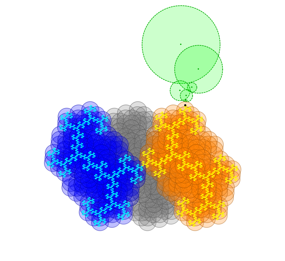
Set where and let be the node in . Observe that is by definition the center of the nodal disk and is a point inside such disk. Therefore, if is far enough from , then , i.e. the reflection of about , will be outside . We can then find an open disk, centered at tangent to (see Figure 3).
Figure 3. Construction of , an element in the connected chain of open sets in . The dotted circle has half the radius of . In order to allow for the existence of , the distance between and must be more than half of the radius of the nodal disk .
Recall that each nodal disk in has a radius of . Thus, the radius, of is easily found to be
We will show that the chain of open disks is a connected subset of the complement of , that accumulates at . The claim of the theorem will then follow from Theorem 4.2(ii), which translates a segment of the chain into a connected, open set of parameter space that accumulates at , and is disjoint from .
Items (i)–(iii) below guarantee that the initial disks of the chain exist, are connected in succession, and are disjoint from the attractor. The proof concludes by using the periodicity of the itinerary of to show that the chain consists of an infinite sequence of re-scaled copies of this initial block, accumulating at .
Each zero coefficient in doubles the size of the overlap set (cf. the note in Section 3). Thus, the condition that is finite implies that all zero coefficients of the power series appear in the first terms (which do not repeat periodically). The choice of which to consider is arbitrary but is always unique because .
We consider only the case to simplify notation. By assumption, the coefficients of are strictly preperiodic, and exactly one of them must be zero (cf. Lemma 3.1). Hence, there exists such that which implies . We deduce that the itinerary of is a word in and, thus, .
Let be such that . Therefore, for all and or (since ). In particular, . Denote by the nodes with itinerary , i.e. . The Taylor polynomial for can then be written as .
Observe that the itinerary of is the (left) shift of by terms. Indeed, we claim that
Since then . Consequently,
The centers of the disks were defined in terms of and , but we can now rewrite them in terms of the Taylor polynomials
Using the above equations, we also rewrite the radius of in terms of a Taylor polynomial:
We are now practically done. For each :
(i)
The disk exists if and only if , namely
which is true by assumption.
(ii)
The disks intersect if and only if , that is
which is true by assumption.
(iii)
The disk is tangent to the nodal disk , where is the itinerary of , by construction. It is disjoint from the rest of the instar if and only if it is disjoint from all other nodal disks; i.e., for every node with and we have . Again, expanding the expressions for and , this means
where is a polynomial of degree at most with coefficients taken from the set . As before, this inequality is true by assumption.
Finally, we claim that for every and . We will show that, after a translation by , the chain is forward invariant under . Therefore, showing that the chain accumulates at .
Observe that and since , then
where the second to last equality is due to the fact that for every .
In particular, is the rescaled copy of , and by part (ii) it intersects non-trivially for all . Theorem 4.1(i) guarantees condition (iii) holds for with .
Hence, the claim follows from Theorem 4.2(ii).
∎
The proof of Theorem 4.5 is analogous, except we only have to show is outside . Therefore, in step (iii) we need to check that does not intersect the instar , rather than .
Remark 5.1.
The conditions of both Theorems 4.3 and 4.5 can be weakened as follows: there exists integers and where such that for all
(i)
(ii)
(iii)
Let be the solution of . Then for any polynomial of degree less or equal to with coefficients in , with it holds that .
These conditions allow the possibility of intersection between two non-consecutive chain disks.
6. Examples: Landmark Points
In [Sol05], Solomyak discussed six sample parameters that satisfy , and named them landmark points. As a note of caution, we changed Solomyak’s nomenclature to tie in with our exposition, so that our correspond to his . In this section we will prove that for satisfy the conditions of Theorems 4.3 and 4.5 and are therefore accessible.
6.1. Period One
The landmark points for are all inside the following sector:
and have itineraries of various preperiods, but all with period . By Proposition 6.1 they are all accessible. Later in Section 6.2 we present a method to circumvent the lengthier computations that would be required to establish the inequalities for (which has period ).
Proposition 6.1.
Let and assume where
is of rational type , that is:
Then satisfies the conditions of Theorem 4.3 (and therefore is accessible).
The proof will use the following properties of :
Lemma 6.2.
For all the following holds:
(a.)
;
(b.)
;
(c.)
;
(d.)
;
(e.)
.
Proof.
From the law of cosines we obtain
It follows that
and
which gives (a.) and (b.).
Similarly,
which gives (c.) and (d.).
Finally,
giving (e.) and concluding the proof of the lemma.
∎
Armed with these inequalities, we proceed to prove the Proposition:
Figure 4. The window of parameter space, showing the sector intersecting and . The landmark points for are marked (we display instead of simply to make a picture with better resolution; see also the footnote to Example 5).
In the following examples recall that the uniqueness of the power series was proved by Solomyak in [Sol05].
Example 1.
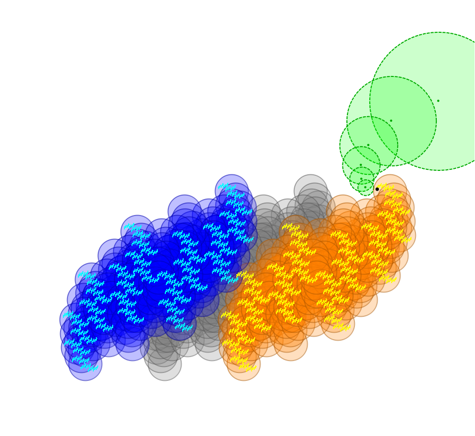
Let and let be the corresponding power series of rational type , that is . The associated parameter in is .
It follows from Proposition 6.1 that the parameter , is an accessible point of (see Figure 5). In fact, by Corollary 4.4, we can conclude that .
Example 2.
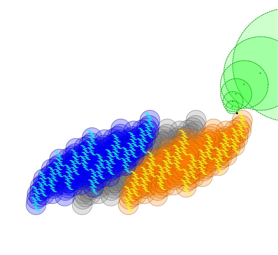
Let and let be the corresponding power series of rational type , that is . The associated parameter in is .
It follows from Proposition 6.1 that the parameter , is an accessible point of (see Figure 5).
Example 3.
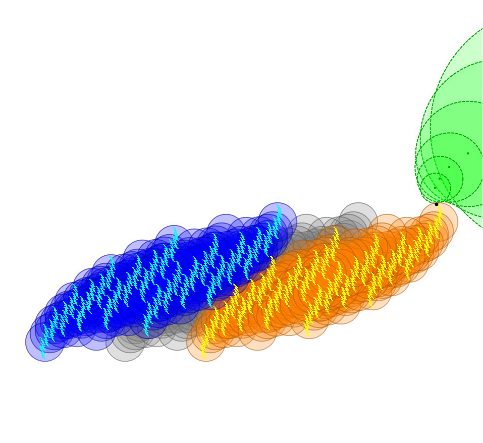
Let and let be the corresponding power series of rational type , that is . The associated parameter in is .
It follows from Proposition 6.1 that the parameter , is an accessible point of (see Figure 5).
Example 4.
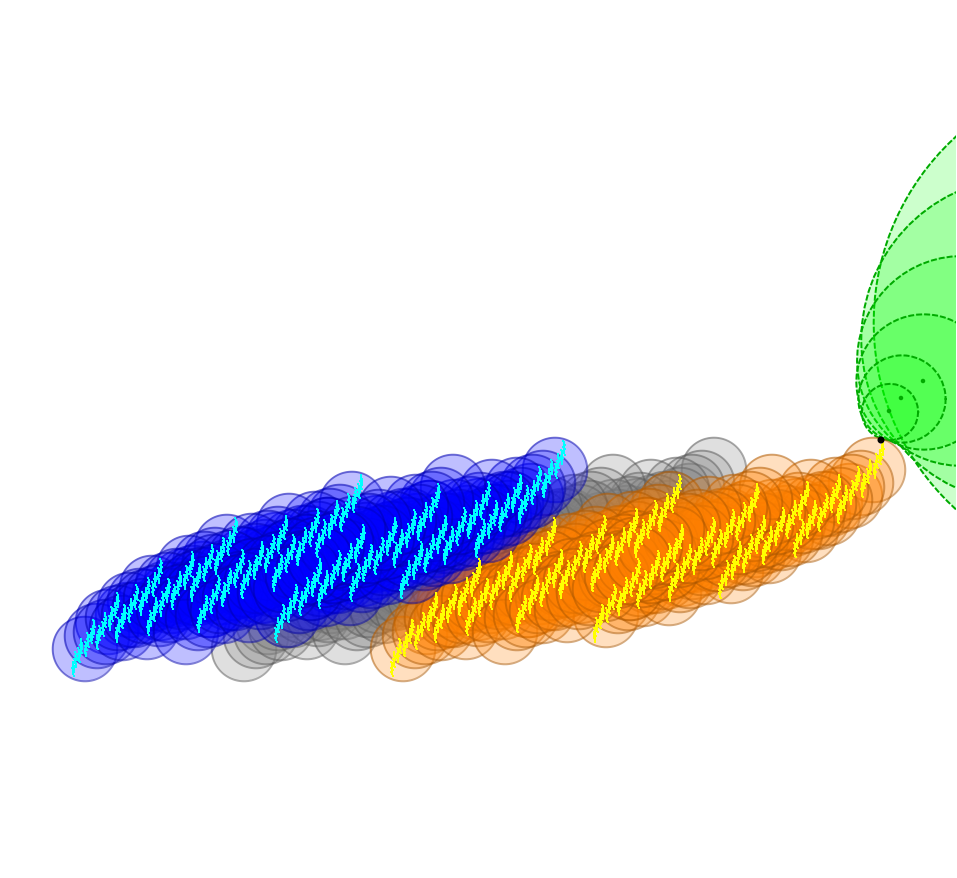
Let and let be the corresponding power series of rational type , that is . The associated parameter in is .
It follows from Proposition 6.1 that the parameter , is an accessible point of (see Figure 5). In fact, by Corollary 4.4, we can conclude that .
Note 6.1.
The overlap set has different cardinalities in each of these examples. In particular, in Example 1 and 4 (where the overlap is a singleton) the parameters belong to both and , whereas in Example 2 and 3 (where the overlap consists of or points) the parameters belong to , but not .
Figure 5. The attractors for (in the order ) inside their respective instars . The green disks in the top-right corners of each plot are part of the chain constructed in Theorem 4.3.
6.2. Higher period
Here we consider the landmark point whose associated itinerary has period . Observe that in this case the number of inequalities to be checked before applying Theorem 4.3 becomes quite large. To overcome this difficulty we rely on the argument and modulus of , and the geometric structure of the instar at each level. We will construct each of the disks of the connected chain that lies in the complement of .
Example 5.
Let and consider the associated power series of rational type . Solomyak proved in [Sol05] that222
Solomyak worked with the word which gives the power series ; in other words, he looked at . The symmetry of allows us to consider instead. is the unique power series for which is a root. Using the notation of Theorem 4.3 we have , , , , and with itinerary .
We begin by proving that the hypothesis (i) of Theorem 4.3 is satisfied:
Lemma 6.3.
Let and be as above. Then for every
Proof.
First notice that
(i)
and
(ii)
.
Then, from (i) we get
From (ii) and the Law of cosines we get
Since then and consequently
because .
∎
Lemma 6.3 guarantees that the disks in the chain exists for every . We can show now that and that , namely the remaining two hypothesis of Theorem 4.3. Recall that each disk is centered at and has radius :
Lemma 6.4.
For , the set is connected and lies in the complement of .
Proof.
By the self-similarity of the attractor at it is enough to prove that is connected and lies outside the instar . We will first show that lies outside the instar and then prove that for each .
:
The instar is the union of the nodal disks , and . We already know that is outside , we want to show that the distances between and the nodes and is larger than the sum of the radii of and the nodal disk of level . In other words, we need that and .
Using that and , the Law of cosines gives
so
Moreover, using the better estimate ,
implying that
:
The instar is the union of the nodal disks , and where . Instead of checking that eight more inequalities are satisfied, we use the fact that to show . Given that we need to check
Indeed, and . Moreover, we have because . Consequently, is in the first quadrant with . It follows that has a chance to intersect only the disks and . However, in Lemma 6.3 we showed that , therefore, since we have
so .
Finally, does not intersect because
In the first equality we used the fact that and in the second line that .
:
In this case we prove that which implies that is outside because of the containment . Firstly, we have and that the radius of is because . Secondly, the radius of is , so for the containment to hold we must have
which holds since .
We have shown that , and do not intersect their respective instar and, therefore, their union lies outside the instar . We have also proved that so it remains to show that and .
We will prove that , i.e. : recall that and then
which implies
Finally, we want to show that .
By definition and since
then
The equality in the third line holds because .
∎
By Lemma 6.4 the chain is connected and lies in the complement of (see Figure 6). Then, by Theorem 4.3, is an accessible point. Because is unique and has no zero coefficients, by Corollary 4.4, is an accessible point of .
Figure 6. The attractor inside . Compare description in Figure 5.
It must be noted that the uncountable set of Theorem 3.3 contains . In fact, such set was found by perturbing the number of repeating coefficients in the power series and by allowing some of the perturbed repeating coefficients to be . The method Bandt and Hung used to prove that no other power series has a root in , entailed finding a uniform lower bound in a neighborhood of on the normalized difference
where and is a power series with a root in . It is unclear whether all parameters in are accessible, since the associated itineraries are not necessarily preperiodic and hence our theorems do not apply.
Remark 6.1.
We want to emphasize that the assumptions of Theorem 4.3 are not meant to be necessary for accessibility. The landmark point satisfies . Based on computer pictures, Bandt [Ban02] describes as the “tip of the largest (visible) spiral of ”. It is likely that is accessible, but even though it is possible to prove that the disks of the chain exist, they are all disconnected and intersect the instar at every level.
Appendix
We are grateful to the anonymous referees for their comments, in particular for the suggestion to add a table of notation. We include that below.
For completeness, the table makes mention of Hutchinson’s operators on , the space of compact sets in . The definitions of attractors and instars in terms of these operators are completely analogous to the approach adopted in this text.
Note further that all entries in the table assume a fixed choice of the parameter , except of course the last row, where parameter spaces are defined.
Generating maps
Hutchinson operators
-attractor
(fixed point of )
-attractor
(fixed point of )
Instars
(, where is a
disk of radius
Overlap set
Power series spaces
Symbolic dynamics
(so that )
Projection
( is the itinerary of in )
Parameter spaces
References
[Ban02]
Christoph Bandt.
On the Mandelbrot set for pairs of linear maps.
Nonlinearity, 15(4):1127–1147, 2002.
[BDLW21]
Harrison Bray, Diana Davis, Kathryn Lindsey, and Chenxi Wu.
The Shape of Thurston’s Master Teapot.
Advances in Mathematics, 377:107481, 2021.
[BH85]
Michael F Barnsley and Andrew N Harrington.
A Mandelbrot set for pairs of linear maps.
Physica D: Nonlinear Phenomena, 15(3):421–432, 1985.
[BH08]
Christoph Bandt and Nguyen Hung.
Self-similar sets with an open set condition and great variety of
overlaps.
Proceedings of the American Mathematical Society,
136(11):3895–3903, 2008.
[Bou88]
Thierry Bousch.
Paires de similitudes, 1988.
[Bou92]
Thierry Bousch.
Connexité locale et par chemins hölderiens pour les systemes
itérés de fonctions, 1992.
[BR07]
Christoph Bandt and Hui Rao.
Topology and separation of self-similar fractals in the plane.
Nonlinearity, 20(6):1463–1474, 2007.
[CKW17]
Danny Calegari, Sarah Koch, and Alden Walker.
Roots, Schottky semigroups, and a proof of Bandt’s conjecture.
Ergodic Theory and Dynamical Systems, 37(8):2487–2555, 2017.
[ERS10]
Kemal Ilgar Eroğlu, Steffen Rohde, and Boris Solomyak.
Quasisymmetric conjugacy between quadratic dynamics and iterated
function systems.
Ergodic Theory and Dynamical Systems, 30(6):1665–1684, 2010.
[HP12]
Peter Haïssinsky and Kevin M. Pilgrim.
Examples of coarse expanding conformal maps.
Discrete Contin. Dyn. Syst., 32(7):2403–2416, 2012.
[Lei90]
Tan Lei.
Similarity between the Mandelbrot set and Julia sets.
Communications in mathematical physics, 134(3):587–617, 1990.
[OP93]
Andrew M. Odlyzko and Bjorn Poonen.
Zeros of polynomials with 0,1 coefficients.
L’Enseign. Math., 39:317–348, 1993.
[Sol05]
Boris Solomyak.
On the ’Mandelbrot set’ for pairs of linear maps: asymptotic
self-similarity.
Nonlinearity, 18(5):1927–1943, 2005.
[Thu14]
William Thurston.
Entropy in dimension one.
Frontiers in Complex Dynamics: In Celebration of John Milnor’s
80th Birthday, pages 339–384, 02 2014.
[Tio20]
Giulio Tiozzo.
Galois conjugates of entropies of real unimodal maps.
International Mathematics Research Notices, 2:607–640, 2020.