What do QAOA energies reveal about graphs?
Abstract
Quantum Approximate Optimization Algorithm (QAOA) [FGG14a] is a hybrid classical-quantum algorithm to approximately solve NP optimization problems such as MAX-CUT. We describe a new application area of QAOA circuits: graph structure discovery. We omit the time-consuming parameter-optimization phase and utilize the dependence of QAOA energy on the graph structure for randomly or judiciously chosen parameters to learn about graphs.
In the first part, following up on Wang et al. [WHJR18] and Brandao et al. [BBF+18] we give explicit formulas. We show that the layer-one QAOA energy for the MAX-CUT problem for three regular graphs carries exactly the information: (# of vertices, # of triangles). We have calculated our explicit formulas differently from [WHJR18], by developing the notion of the -polynomial of a graph . Many of our discoveries can be interpreted as computing under various restrictions.
The most basic question when comparing the structure of two graphs is if they are isomorphic or not. We find that the QAOA energies separate all non-isomorphic three-regular graphs up to size 18, all strongly regular graphs up to size 26 and the Praust and the smallest Miyazaki examples. We observe that the QAOA energy values can be also used as a proxy to how much graphs differ. Unfortunately, we have also found a sequence of non-isomorphic pairs of graphs, for which the energy gap seems to shrink at an exponential rate as the size grows. Our negative findings however come with a surprise: if the QAOA energies do not measurably separate between two graphs, then both of their energy landscapes must be extremely flat (indistinguishable from constant), already when the number of QAOA layers is intermediately large. This holds due to a remarkable uncoupling phenomenon that we have only deduced from computer simulation.
To compute average values of QAOA energies and their standard deviation for a large number of levels, we introduce QAOA dynamics, and discover a tool for studying it: higher order density matrices.
Alibaba Quantum Laboratory, Alibaba Group USA, Bellevue, WA 98004, USA
Dedicated to the 70th birthday of Laci Babai
1 Introduction
Quantum Approximate Optimization Algorithm (QAOA), introduced by Farhi, Goldstone and Gutmann [FGG14a] in 2014, is an attempt to gain quantum advantage in solving combinatorial optimization problems of the form
with a quantum machine in the circuit-based (as opposed to annealing-based) computational model. In this article we shall only be concerned with the special case, where we have an undirected graph and
| (1) |
, but we omit the subscript when it does not cause ambiguity. When minimized, this gives a maximum cut of via
Although the problem is classical, Farhi et al. construct a quantum circuit, called the QAOA circuit, that spits out good approximate solutions when its parameters are optimized. The optimization process is known as the QAOA optimization phase. It is a loop where the QAOA circuit is repeatedly run, its output is evaluated and the circuit parameters are reset. When the final parameter values are reached, the circuit is run a few more times to produce a set of candidate assignments to the optimization problem. Finally, the best of all candidates is chosen. The algorithm has become the most frequently discussed quantum-classical hybrid algorithm [MRBAG16].
More into the details, the level- QAOA circuit for a graph and for parameters , computes an -qubit quantum state , where , and
| (2) |
The product outside is responsible for making the levels. Since a single level is composed of two operators (the two products inside), it is tempting to think that the usual circuit depth of the level- QAOA circuit is . Although has depth one when presented as a quantum circuit, the depth of is typically not one, and finding the smallest depth implementation requires graph theory. All 2-qubit gates of the form commute, but they share qubits. One has to refer to the Vizing theorem to get a depth rendering of these gates in the worst case (and depth in the best case), where is the maximum degree of . All-in-all we get a depth upper bound for the entire circuit.
Although is treated as the quantum Hamiltonian , the ground energy, , is achieved at a classical state because of the diagonal form of the Hamiltonian. Nevertheless, the QAOA circuit produces a quantum state, and this is precisely where its strength lies: it adds a quantum dimension to an otherwise classical problem.
The QAOA circuit is also called an “Ansatz,” i.e. “rudiment” or “approach,” meaning that it only gets us started solving the optimization problem . The remaining task is to choose the parameter values , called angle sequences, in an optimal way. The optimized state is mathematically guaranteed to converge into the subspace spanned by the optimal classical solutions ([FGG14a], Section VI), but the rate of convergence may be very slow. For small , even after setting the parameters in the most optimal way, we may end up with a low-quality solution.
Graph structure discovery. We harness the “quantum dimension” present in the QAOA Ansatz in a new way: to obtain information about the structure of the input graph, via the quantum object in (2), which is supposed to encode main features of the graph.
Definition 1.
We denote the state in (2) with where and .
Instead of looking to solve the optimization problem in (17), our main goal is to understand
for random or arbitrary . We compare energy values for pairs or sets of graphs for identical degree sequences. Our investigation has started from a conjecture which is still unresolved:
Conjecture 2.
Let and be two non-isomorphic graphs. Then for some , when is randomly and uniformly chosen from we have
An analogous statement in the case of boson sampling is proven in [BFI+18, SBI+19]. To turn Conjecture 2 to an even stronger conjecture of quantum polynomial time graph isomorphism algorithm, the separation must be at least inverse polynomial for random degree sequences, and must be polynomial in the size of the graph.
In the first part of the paper we ask: what features of a graph are encoded in ? We show:
Theorem 3.
Let and . Then for any cubic graph with nodes and triangles:
-polynomials. We have developed this tool to prove Theorem 3, but it was useful in all our calculations. One might view -polynomials of a graphs as certain types of tensor-networks or partition functions for certain Ising models. The notion’s advantage is a graph theory- friendly language. We defer all information about -polynomials, including their definition, to the appendix.
Unlike in the first part of the paper, where all statements were mathematically verified, in the second part, aside from the last section, we rely on computer experiments. We show that single random QAOA energies can already distinguish all non-isomorphic members of large classes of graphs such as all 3-regular graphs of size 16. Unfortunately, it also seems, that polynomial time graph isomorphism testing with QAOA is unlikely: the family of pairs of graphs seems to exhibit an exponentially shrinking sequence of average energy gaps. The average energy gap for two graphs, and is defined as
Our hard graph pairs may also disqualify annealer-based graph isomorphism testers as in [HY12], and it could be interesting to analyze them for boson sampling-based testers as well.
We have found an interesting consequence of small energy gaps: due to a numerical observation what we call a decoupling phenomenon (see Section 13), small at large implies flat energy landscapes for both graphs. This in turn has hardness consequences on optimization.
There is a good news too: we have evidence that QAOA energy differences can be useful to detect “intuitive” graph similarity. Graph similarity is a measure that exists between any two graphs. In [SA19, SSL19] similarity is rigorously defined as the graph edit distance. In our article we have avoided the expensive graph edit distance calculations by replacing it with studying a Markov chain on graphs that makes a small local change at every step. We observe that the average QAOA energy gap between graphs that are farther in this walk is larger.
In the third part we develop methods that mathematically address questions raised in the second part. The quantity
| (3) |
is easier to analyze than , so we will focus on . We assume that is large, which lets us focus on:
The QAOA dynamics. Let be an arbitrary graph. A QAOA circuit for with random angles and with increasing depth can be made a Markov chain on the dimensional complex unit ball, , with the transition rule:
Apply a new level of the QAOA circuit with random angles.
After each step we have updated the statistical ensemble of states on qubits, which seems to weakly converge to a limiting distribution, , on . This gives rise to new graph parameters:
The QAOA moments of are defined as . The decoupling phenomenon, described in Section 13, gives
| (4) |
reducing the gap-question to the calculation of and of graphs. We provide a methodology for such a calculation in the form of higher order density matrices. We demonstrate the use of this tool by calculating some first and second QAOA moments for small graphs.
Part I Explicit Formulas
The QAOA research has been taking diverse directions. A lot of emphasis is put on issues such as advantage over classical [FGG14b, FH16, Has19], noise sensitivity [AASG19], parameter optimization [ZWC+18, SA19, SSL19, Cro18], implementation [PMS+14, GM19], simulation [ZHN+19].
The QAOA energy values more often than not are calculated by computer simulation. There are also exceptions, most notably by Wang et al. [WHJR18] and Brandao et al. [BBF+18], who make exact calculations. We follow their tradition and provide a number of explicit formulas for special cases.
2 Level-1: All graphs (Wang et al.)
We adopt the following result from Wang et al [WHJR18] (modified for our notations and corrected a typo). Let , and be the number of nodes that are connected only to the left, only to the right and to both nodes of an edge of . Then the level one QAOA energy associated with edge of and rotation angles is:
![[Uncaptioned image]](1912.12277v2/degrees.png)
|
From this we get that the energy of every edge of the cycle with :
More generally, the energy contribution of every edge of a triangle-free -regular graphs is
yielding when summing it up for all edges.
3 The Triangle Theorem
 |
 |
 | ||
| type 0 | type 1 | type 2 |
In this section we prove Theorem 3, which we call the Triangle Theorem, which states that the level one QAOA energy of a three regular graph is:
| (5) |
Since is three regular, we may encounter three different types of neighborhoods at edge-distance one as in Figure 1. Let , and count the number of edges of with these neighborhood types. These three parameters already determine the level one QAOA energy of cubic graphs as noted in [BBF+18]. Let the single edge energy associated with type be . Then the total energy is
| (6) |
We replace , and with just and . That we can do this is due to a co-incidence:
Lemma 4.
Proof.
From the displayed expression of the previous section we can express , and :
| (7) | |||||
| (8) | |||||
| (9) |
To verify all we have to show is that
which can be easily seen from that both sides are .∎
Now we can eliminate from Equation (6):
| (10) |
By counting the edges of all triangles in two different ways we get:
| (11) |
which together with Equation (10) gives us
since the number of edges of is , as is 3-regular. Now Equations (7) and (8) and basic trigonometric identities immediately give Theorem 3.
4 Level Two: Cycles
The MAX-CUT QAOA expressions for level-2 have significant complexity. We have calculated the expression of the single edge-energy for cycles of length at least 6 to get an idea about its form and complexity. We could put the expression into other equivalent forms but they were not simpler. In [WHJR18] a significantly more complicated formula is given.
The 2-level QAOA energy for in with angle sequence :
The QAOA energy of a -cycle is simply times the above amount.
5 Analysis of the single-edge graph
Formulas for level two QAOA are complex, but level seems nearly intractable. Here even the graph containing a single edge is a challenge. The straightforward state evolution for a sequence gives the final state
where
and . Once the state is iteratively computed for level , the energy is . Interestingly, we can come up with a different (although similar) formula that avoids taking the squares when computing the energy. Let
be a starting vector. Define Matrices
Then the energy value can be expressed as
It is worthwhile to write out (for ).
It is easy to see that
We can repeatedly apply the above, starting from , to get:
Lemma 5.
The expected QAOA energy of a graph containing a single edge is for every .
The lemma does not imply, that the average QAOA energy of every graph is . Experiments show that is not always the average energy, but it is a good approximation.
6 Examples
 |
 | |
| a.) Test graph | b.) Grid implementation of |
Assume we want to validate the QAOA algorithm on a quantum chip with an 8 by 8 grid architecture. Since this is our first test of the device, we want to choose a graph with low degree to reduce the circuit depth. The architecture for instance allows to embed a cycle of length 64 without intersection. We use the formula in Section 2 to get the level one QAOA energy
Another example is the graph shown in Figure 2/a, which is 3-regular. The nice thing about is that it can be implemented on the 8 by 8 grid as shown in Figure 2/b. For a diagonal edge the operation can be performed as
where form a right triangle (the grid edges replacing the diagonal edges are dashed red in Figure 2/b). The graph has 48 nodes and 16 triangles, therefore its level one QAOA energy is
Further, if we set the formula gives 42. In contrast, a random assignment would give energy 72/2 = 36, on expectation.
Part II Graph Similarity and Graph Isomorphism
7 Algorithm
Our fundamental algorithm computes the QAOA energies of a set of graphs (often just and ) with respect to the same random degree sequences
If two graphs are isomorphic, their energies are the same for the same . Our experiments indicate that if two graphs are not isomorphic, their energies differ for some large enough . The indication is admittedly weak: we have not found any counter-example in spite of probing large families of graphs as well as some specific hard pairs. The smallest , which separates all graphs on nodes, which is not ruled out by our trials is . It would be surprising if more levels than a small constant times the number of edges (or even nodes) was necessary to separate any pair of connected graphs, if they are separable at all. Conjecture 2 expresses our belief that QAOA energies distinguish non-isomorphic graphs. This is one of our motivating questions. An even bigger question is if the energy gaps are large enough to be detectable with a quantum computer. As we shall see, we have counter-indications for that.
For our experiments we have computed the QAOA energies of all graphs with a classical simulator. Double precision was sufficient for us, although theoretically, with a polynomial factor overhead, we could have afforded computing all values with polynomially many digits of precision. In classical simulations the bottleneck is not the precision, but that the number of arithmetic operations grows exponentially with even for polynomial . As long as we are satisfied with logarithmic digits of precision, i.e. with an additive output error, an estimator of can be computed with a quantum computer for graphs with nodes and with levels. This is stated, among others, in [FH16], and the underlying algorithm is really simple:
...............................................................
...............................................................
Here , the number of repetitions, is a parameter of the algorithm, which must be sufficiently large. If the fidelity of the circuit-output is , then for an actual output we have . Then , when , showing that a circuit with fidelity inverse polynomially close to 1 still works sufficiently well.
8 The Cost of Communicating Isomorphism of Graphs
Consider the problem where Alice gets a graph , Bob gets , both on nodes, and they want to find out if is isomorphic to . If the only resource we care about is the communication cost between Alice and Bob, there is a constant bit 1% error protocol in the public coin setting, where a random string is given to both Alice and Bob (at no cost) before their exchange begins.
We will show how to reduce the problem to the following famous public coin communication protocol for the Equality function:
In this protocol both Alice and Bob get a random string . Then Alice sends over the modulo two inner product of and to Bob, who in turn outputs 1 if and 0 otherwise. The protocol always succeeds when the two strings are equal, and if not, it will be revealed with probability 0.5. With a constant number of repetitions the probability of failure can be reduced to below 1%.
At first the graph isomorphism problem seems much harder, since Alice and Bob have to deal with an unknown isomorphism between their respective input graphs. The predicate can only reveal if and are written down in the same exact way. There is a way however to get around this problem. The idea is that Alice and Bob first independently bring their graphs into their respective canonical forms. A canonical form is a map from graphs to strings with the property that for two graphs, and we have if and only if the two graphs are isomorphic. Since graph isomorphism is an equivalence relation, such a map exists. The protocol fixes this map, and Alice and Bob are left to solve with constant bits of communication (the communication is constant even if is exponential).
The problem becomes much harder if we are also concerned with the cost of computing . Laci Babai in a recent work has given a function computable in time [Bab19a]. Such a function also solves the graph isomorphism problem in time , but the converse is not straightforward, and in fact three years have elapsed between results [Bab19a] and [Bab16], where the first quasi-polynomial graph isomorphism algorithm was introduced.
The QAOA Ansatz for the MAXCUT problem of offers a way to construct a randomized map that canonically encodes graphs, conditional to Conjecture 2, when is sufficiently large. The associated protocol is:
...............................................................
...............................................................
In most (but unlikely in all) cases, separates two non-isomorphic graphs with high probability even if we do the computation only with logarithmically many bits of precision. In such cases we can replace with estimator , computed by the quantum algorithm of the previous section. Further, the energy values and need not be further composed with if we are satisfied with logarithmic bits of communication between Alice and Bob. The QAOA map itself behaves as a kernel function, something like the inner product in the EQ protocol. The following analogy might be enlightening:
Alice is given and Bob is given . Construct a time- and communication- efficient randomized communication protocol that finds out if and contain the same elements of , each the same number of times
In the trivial solution Alice and Bob privately sort their input with multiple occurrences kept (hence both computing “the” canonical form of their respective sequences) and then apply the EQ protocol for the sorted sequences. There is a different protocol however, where a random is used. Alice sends over to Bob, who then compares this with , and outputs 1 if the two numbers are equal. We consider this protocol as the smaller brother of our QAOA based algorithm for graph isomorphism. It turns out that the above protocol for identifying multi-sets already performs well, when the numbers are calculated with digits of precision.
Further, it is not hard to see a connection between the above formulas and characteristic functions of probability theory. It would be worthwhile to explore if probability theory could take any use of QAOA energies or related formulas.
9 Graph Isomorphism and Quantum
Utilizing the power of quantum in the context of the graph isomorphism (GI) problem has been put forward in many works. Since the GI problem shares some common traits with the integer factoring problem, researchers sense here yet another spectacular demonstration of quantum advantage. Nevertheless, there are reasons to be cautious. Although both GI and factoring can be viewed as special cases of the hidden subgroup problem, the two problems behave differently. The GI problem (classically) is very easy on average: An early result of L. Babai, P. Erdős and S. M. Selkow [BES80] shows that a straightforward linear time canonical labeling algorithm applies to almost all graphs. The worst case classical complexity of GI is [Bab16], while factoring seems to require time for some , possibly . Interestingly, while GI is relatively easy classically, it seems to resist the hidden subgroup problem approach, while the harder factoring yields to it.
A different quantum approach to GI is to look for quantum-computable graph invariants [MRS+19, ZPDF16]. A prospective way of obtaining a full set of graph-invariants, i.e. an array of graph parameters that separate between any two non-isomorphic graphs, is via quantum walks. In a broader sense both [MRS+19] and QAOA qualify as -particle quantum walks. In [GFZ+10] it is experimentally shown that quantum walks of two interacting particles can successfully distinguish between some strongly regular graph pairs that single particle walks or non-interacting particle walks provably cannot. Similar results were obtained by S. D. Berry and J. B. Wang [BW11]. Godzil and Guo [GG11] calculate spectra of quantum walk operators, but they do not conclude that two interactive particle walks always distinguish non-isomorphic strongly regular graphs. J. Smith has a publication in the arXiv entitled “k-Boson quantum walks do not distinguish arbitrary graphs” [Smi10]. I. Hen and A.P. Young have experimentally tested a quantum annealing based graph isomorphism tester [HY12] with some satisfying outcomes, but the authors also express: “The results we presented here support a conjecture that the Quantum Adiabatic prescription can differentiate between all non-isomorphic graphs, given an appropriate choice of problem and driver Hamiltonians. This conjecture needs to be tested more thoroughly, both theoretically and also by experiments on real quantum annealers.” We think, that if our algorithm does not work, there is little chance the annealing based algorithm will, since QAOA was distilled from the former. The same pairs may fool both. The work of D. Tamascelli and L. Zanetti [TZ14] is different from the previous ones, in that it starts with an equivalent rewriting of the graph isomorphism problem as an optimization problem, so there is a guarantee that their algorithm succeeds. The question is however the running time, that can easily be exponential.
In a sequence of innovative works by Xanudu reserchers K. Bradler, S. Friedland, J. Izaac, N. Killoran, and D. Su [BFI+18] and later M. Schuld, K. Bradler, R. Israel, D. Su, and B. Gupt [SBI+19] the authors identify graphs encoded in quantum state of light. They show that photon states encoding non-isomorphic graphs give different detection probabilities. What remains is to upper bound the size of their sampler and to lower bound the gap in the statistics.
10 Graph Similarity and QAOA energies

Even if our QAOA-based algorithms fail to detect graph isomorphism, they might still recognize if two graphs are similar. What is graph similarity?
The QAOA energy-gap dependence from graph edit distance between pairs of graphs was studied in [SA19, SSL19]. Isomorphic graphs have graph edit distance zero. In general, graph edit distance between graphs and is the length of the shortest add-delete sequence of edges that takes to some isomorphic copy of . This distance is a metric. Shaydulin et al. have looked at how the maximal QAOA energy and optimal angle sequences are different for graphs that are close in graph edit distance. They have found that graph edit distance is a good predictor whether these differences are small or large. Our pursuits differ from the above research in three ways:
- 1.
Our goal is not to find or estimate optimal QAOA angles, but rather to use QAOA to detect graph similarity.
- 2.
We do not compare energies at optimal angles, but rather at random angles.
- 3.
For our experiments we do not go through the hard task of computing graph edit distances. Rather, we are satisfied with a more heuristic method. We have designed a random walk on -regular graphs such that each step changes the graph edit distance by at most four. We expect that starting from any graph, as we walk away from it and plot the QAOA energy differences, they grow.
We have found energy difference that increases with the walk-length and eventually reaches a plateau, which is probably due to the walk mixing into random graphs.

11 Landscapes


A graph similarity measure is a metric on all or on a select set of graphs. When this metric can be embedded into , we can draw a visual image of how the graphs in our set (like all 3-regular graphs of a given size) cluster according to the metric. We call such an embedding a landscape, which is not to be confused with energy landscapes. Our landscapes are graph landscapes.
Graph landscapes made from QAOA energies reveal intriguing properties of graphs. Consider for instance the , the set of all 3-regular graphs with 16 nodes. Let , and fix . Define the map by
Figure 5 (b) and (c) show two such landscapes made from different angle sequences. The clusters are clearly visible in both. Closer examination has revealed that the dominant clusters are formed by graphs with the same number of triangles. We have colored some subsets that contain graphs with the same number of triangles with different colors. Each color except the green corresponds to a fixed number of triangles.
The dependence on the number of triangles is even more revealing when . Figure 5 (a) shows such a landscape of all three regular graphs with 14 nodes. The clusters shrink to a single point, which hints at Theorem 3, and in fact this is how we have discovered it. The same structure is not true for 4-regular graphs any more, and we need more graph invariants to explain the landscape.
12 What are the least distinguishable pairs of graphs?
 |
 |
 |
 | |||
Heuristic algorithms for the graph isomorphism problem are often tried on easily confusable graph pairs [NS17]. According to Laci Babai, only the most naive algorithms fall victim to strongly regular graphs with the same parameters or to iso-spectral pairs. The Cai-Furer-Immerman [CFI92] and Miyazaki graph pairs [Miy95, TD11, NS18] are a more serious challenge [Bab19b].
For different GI heuristics different graph pairs are hard to distinguish [MRS+19]. We have tested our algorithm on Miyazaki-inspired small examples, and on 20 nodes (Figure 7, right two), each level from one to ten with 5000 random probes. For our pair there was no gap up-to level 2. The separation has occurred at level 3:
| level () | 2 | 3 | 4 | 5 | 6 | 7 | 8 | 9 | 10 |
|---|---|---|---|---|---|---|---|---|---|
| gap | 0 | 0.0003 | 0.0012 | 0.0026 | 0.0037 | 0.0054 | 0.0069 | 0.0083 | 0.0094 |
| squared | 0 | 1.7e-06 | 1.2e-05 | 3.4e-05 | 5.4e-05 | 9.4e-05 | 1.3e-04 | 1.7e-04 | 2.0e-04 |
While plotting the landscape for all connected 3-regular graphs with 16 nodes for levels one, two and three we have noted that among all 4060 non-isomorphic three regular graphs, when reaching level three, only a single pair of graphs remained that always had the same QAOA energies. We have discovered that these two graphs were the Circular Lattice () and the Moebius Lattice () (Figure 7, left two). This can be explained by that the edge-neighborhoods of and are the same. Following this clue we have examined the average gap from to at level 60 (maximal gap seems to be reached at levels already, so we do not expect better separation for and ). and we have found the sequence exponentially decreasing.
| size parameter () | 3 | 4 | 5 | 6 | 7 | 8 | 9 | 10 | 11 |
|---|---|---|---|---|---|---|---|---|---|
| 1.07 | 0.81 | 0.47 | 0.283 | 0.182 | 0.1025 | 0.062 | 0.0337 | 0.015 | |
| ratio to the previous | N/A | 0.757 | 0.58 | 0.602 | 0.638 | 0.563 | 0.604 | 0.544 | 0.445 |
This table gives us the strongest evidence so far that a QAOA-based graph isomorphism tester may not work.
13 A Decoupling Phenomenon
 |
 | |
| (Circular, Moebius) (16 nodes) | (Praust1, Praust2) (20 nodes) | |
| blue = uncorrelated; orange = identical | blue = uncorrelated; orange = identical | |
 |
 | |
| (6-cycle, ) (6 nodes) | (4-path, 3-star) (4 nodes) | |
| blue = uncorrelated; orange = identical | blue = uncorrelated; orange = identical |
We have arrived at one of the most surprising findings of this research, which we have only experimentally asserted. Let and be two non-isomorphic graphs. We have considered the expected energy difference for randomly chosen in :
where was . Then we have computed similar expectations, where we randomly and independently picked and in :
What we have found is
In other words, the QAOA energy of decouples from that of as we probe them on longer and longer identical angle sequences (of course only when graphs and are not isomorphic).
The expression is uniquely determined by the distributions of and alone. But the expectation, , of the squared differences is easier to compute from these distributions than :
| (16) |
where and are the following expectation values for uniformly random in :
In the last (third) part of the paper is what we are going to analyze by finding ways to compute , , and . Equation (16) turns out to have an interesting consequence if is “exponentially” small (like ). Since
the energy landscapes of both and at level are extremely flat.
14 Efficient graph isomorphism with QAOA? – an assessment
Even if QAOA energies of non-isomorphic graphs differ for randomly chosen degree sequences and for large enough as Conjecture 2 hypothesizes, we are not guaranteed to have a polynomial time quantum algorithm for testing graph isomorphism, because the energy gap may be too small or may be too large. In Section 12 we have unfortunately seen indications for the former. Below we formulate a sufficient condition for efficient isomorphism testing (under the usual circuit model, which is also the model for Shor’s algorithm).
Theorem 6.
Assume that there are polynomials and such that for any two graphs and on nodes there exists some such that
Then our main algorithm in Section 7 can be turned into a quantum-polynomial time graph isomorphism solver.
Proof.
First, it is a minor issue that the theorem does not assume the knowledge of , since we can just try all . The level- QAOA circuits for and have at most gates. With error correction, each gate as well as the input preparation and the final measurement can be implemented with fidelity, where we choose
Then, the fidelity of the entire circuit is not less than . The QAOA energies of and are upper bounded by , so by Markov’s inequality the probability that for a random degree sequence the QAOA energy difference of and is at least is at least . The fidelity of the output enables us to compute the QAOA energy of both and for a given degree sequence with at least precision in fraction of the time, where can be made any inverse polynomial (by sampling the energy sufficiently many times for the degree sequence in question).
Set and run the distinguisher on random degree sequences. Here is a user-defined number, where the user wants to achieve error rate for the algorithm. Analyse the cases:
Case 1: and are isomorphic. In this case the true energy difference is zero for all degree sequences. By the in union bound the probability that we turn up something larger than in rounds (the rounds correspond to different random degree sequences) is at most for and the same for , so the probability of failure is at most .
Case 2: and are not isomorphic. In this case the probes must hit the set of angle sequences where the energy difference is at least at least once (but typically times) with probability . When this happens, the algorithm may fail to output an energy difference or greater with probability at most . So the error probability in this case is again at most . ∎
A similar argument lets us replace with (the expectation of squared energy differences). Next we look at the indications and counter-indications that the conditions of Theorems 6 holds.
14.1 Indications and counter indications
Our original hope of building an efficient QAOA-based graph isomorphism tester was based upon that we could separate all non-isomorphic pairs of graphs that our QAOA simulator could handle, and even entire classes, like all 3-regular graphs up to 18 nodes and strongly regular classes up to 26 nodes. Further, the separation usually happened already at a very low QAOA level:
| Class or Pair of Graphs | QAOA Depth Giving Full Separation |
|---|---|
| Myazaki I and II, 20 nodes | 4 |
| Praust I and II, 20 nodes | 4 |
| All 4060 non-iso 3-regular graphs | 4 |
| All 41301 non-iso 3-regular graphs on 18 nodes | 4 |
| All 10 non-iso graphs in the SRG 26,10,3,4 family | 3 |
Another indication that the number of levels will not be an issue, is that very quickly converges in terms of , and even quicker becomes convex in all examples we have looked at. Therefore, we do not anticipate any problem with Conjecture 2, and we also believe that the number of levels where the separation happens is bounded by a polynomial. If the conjecture is proven, it would be an analogue of the photon state -based tester result in [BFI+18].
The issue is the energy gap. For a pair of graphs let us set large enough that the expected gap almost reaches the plateau (our experience is that the gap stabilizes as grows, and that a polynomial is sufficient). We consider families of pairs of graphs. Upon recognizing that the (Circular Ladder, Moebius Ladder)n family can be a counter example, we started to work on proving that the (best) gap is exponentially shrinking. We suspected that already the much simpler cycle sequence (, )n shows the behavior. That has turned out to be false – somewhat of a positive sign.
The uncoupling phenomenon has raised hopes once again: exponentially small un-coupled gap between two graphs would imply that the QAOA energy is very close to constant for both graphs. Surprisingly, however, our numerics strongly suggests that large circular ladders have indeed extremely flat energy landscapes.
14.2 A no-go theorem for hyper-graphs
Undoubtedly the most concrete evidence against a polynomial (or even quasi-polynomial) time QAOA-based graph isomorphism tester is that the energy gaps between the Ladder and the corresponding Moebius Ladder graphs seem to be exponentially shrinking. Not only that, but the shrinkage factor seems to even grow slightly (Figure 8). This is not the only counter-indication. An abstract look at the problem yields that certain proof methods must fail.
MAXCUT is just one of the many problems to which QAOA applies. Encouraged by the distinguishing power of QAOA on small MAXCUT instances we might try it on small combinatorial structures other than graphs.
Weighted Constraint Satisfaction problems (WCSP). A WCSP instance on bits is a set of -local constraints, i.e. each is a function that depends on of the bits. The task is again to find an -bit assignment that minimizes .
The QAOA circuits are analogous to those made for MAXCUT, except instead of two-qubit gates we have -qubit gates . Unfortunately, there are two 6-bit non-isomorphic WCSPs that for all degree sequences give the exact same energy values. This is unlike the behavior of MAXCUT QAOA, where we have not found two non-isomorphic graphs so far with the exact same energy values for all .
The counter-example is a pair of systems, we call them and , each with , and each with a single constraint. These instances are not even “weighted” in the sense that their constraints are either satisfied by a assignment, i.e. return 1 or are not, i.e. return 0.
The single constraint of is satisfied by those 6-tuples that have weight 2, and each satisfying assignment is the indicator function of an edge in a union of two disjoint triangles. is similar, but the satisfying assignments are indicator functions of edges of a six-cycle. These instances should not be confused with MAX-CUT graph instances. In particular, the energy of an assignment for and is always either zero or one depending on whether is among the satisfying assignments or not. In contrast, the MAX-CUT energy for an assignment is the number of edges of the input graph that the assignment does not cut.
To compute the QAOA energies we use the Feynman path approach. A Feynman path for the level QAOA is a sequence
where is the number of bits of the instance. The path corresponds to an up-going input-output path of the QAOA circuit. To calculate the amplitude associated with this path, let us notice that each picks up a phase , where is the energy associated with by the (diagonal) instance Hamiltonian, and the transition has amplitude
Here we are concerned only with the instances and , so is either 0 or 1. When computing the QAOA energy we sum up the amplitude squares for all the paths that terminate in any with . To compute the amplitude square, for every such we need to consider products of pairs of such paths, the second component conjugated. Thus, if is any of or :
| (17) |
where
What makes the QAOA energies the same for and is that one can find a one-one correspondence between their Feynman paths pairs with the same contribution.
To define such a correspondence, let be the set of assignments with Hamming weight . Let be either or . For every and there turns out to be a unique number, , that tells how many ways one find for an with , that is fixed in advance (it turns out, all choices of give the same numbers), such that
- 1.
- 2.
Not only that does not depend on the choice of , but it does not depend on whether is or . So we set . Here we list some of the values of :
We leave it to the reader to verify that the existence of such an is sufficient to match up the terms in Equation (17) for and (hint: parse from left to right, and find a match by iteratively matching the s and s).
Part III The QAOA Dynamics
The research in part has grown out of the following problem:
Prove or disprove the observed exponential decrease of the average energy gap
(Table 8)
for the Circular vs. Moebius Ladder pairs.
In Table 8 was chosen, but in general we want to pick a which increases as the instances increase. According to our experiments, for any pair of graphs the energy gap stabilizes rather quickly, and we have never seen any violation of
Similar observation holds for the easier to handle quantity. Due to the hypothesized Equation (3), estimating the latter reduces to estimating QAOA moments, at least for large enough . Let us elaborate on this. In the introduction we have informally defined the QAOA dynamics. We now define it formally.
QAOA Dynamics Let be a graph on nodes. We shall denote probability distributions on the set of qubit pure states, by upper case sigmas. We stick to the usual system of notations in probability theory and treat just as a set. Thus, for a probability measure on the notation for returns the infinitesimal measure that assigns to , that can be only used inside an integral. The stochastic map that takes a distribution on to a new distribution on when we add a new level of QAOA with random angles, is a random mixture of unitaries:
(18)
In the dual form, let be a probability measure on . Then for :
(19)
uniquely defines in the sense that it tells how to integrate over . Let be the distribution, which is concentrated on (the zeroth layer QAOA). We conjecture that the QAOA dynamics takes to a limiting distribution as tends to infinity:
Conjecture 7.
The limiting distribution exists.
Remark 8.
The weakest notion of limit that is still useful for us is via the weak convergence of measures. We require that for all bounded, continuous functions on the dimensional complex unit sphere exists and equals to .
We shall accept Conjecture 7 as true in the sequel.
15 On von Neumann’s Simplification of Statistical Ensembles
A basic tenet of quantum information theory, that goes back to von Neumann, states that when we see a probability distribution on pure quantum states , we can turn the object into the density matrix without losing information that matters. This is true in most settings, but because in our study statistical ensembles
arise differently from how they arise in physics, we cannot use the simplification rule of von Neumann without further ado.
Let us clearly state the dos and don’ts. Assume Alice has a machine with a red button, which when Bob pushes, he uniformly gets either or . Let she have another machine , which looks exactly like , but upon the push of the button Bob uniformly gets either or . Then there is no way Bob could distinguish between the two machines, however long he plays with them, since the output of both are expressed with the same density matrix:
No matter how many times Bob tries the buttons, no matter what measurements he performs on the output states, he remains un-informed about whether he holds or .
Let us now give Bob the supernatural power that when he gets a (pure) state , he can compute the energy value associated with the Hamiltonian
| (20) |
Then whether he holds or is no secret anymore. Even pushing the button only once, if the energy is either zero or one, Bob holds the first machine, and if it is he holds the second. If he pushes the button 6 times he will measure energy values something like () versus ().
Alice can easily give Bob the power of computing . She just installs a blue button on her quantum computer, which when Bob pushes, he gets the exact same pure state as in the previous run. Then by a few applications of the blue button Bob can do a full state tomography on , which in turn lets him estimate . In contrast, in physics experiments the randomness that selects a pure state from a set of pure states (thus yielding a mixed state) cannot be replicated and remembered: it is not under the control of the experimental device.
One can use the density matrix formalism if and only if the randomness creating the mixture is inaccessible and not replicable.
Note: When showing this section to D. Ding, he has pointed out that S. Popescu in [Pop18] describes a thought experiment leading to a very similar conclusion: any knowledge about the preparation of a statistical ensemble renders the density matrix formalism insufficient.
16 Higher Order Density Matrices
Our goal will be to compute the variance of the QAOA energy values over random angle sequences when the graph and the level are fixed. If the angle sequence is also fixed, we have a pure QAOA state. By randomizing over angle sequences we have created a statistical ensemble out of these pure states. This is a continuous ensemble, but for simplicity in this section we formulate everything in terms of discrete ensembles. Our definitions easily carry over to continuous ensembles.
Assume we have a statistical ensemble of pure states, and a Hamiltonian on the same Hilbert space. What information about the ensemble is sufficient to compute the variance of the random variable defined by:
The first thought would be that this should only depend on the density matrix, . In particular, we may have the illusion that what we are really computing is
But not! only if each is an eigenstate of . Otherwise we have to subtract the non-negative quantity from to get , or do a direct calculation to arrive at:
We focus on the expression , since this is what requires explanation. The example in the previous section can be pushed one step further to show that is insufficient to express (see example in the end of this section). Thus we also define
Warning: In general , where is the usual (first order) density matrix. The point of introducing is exactly that it carries information about the ensemble that does not.
Remark 9.
Higher order density matrices are a tool in quantum chemistry where we trace out all but electrons from an -electron wave function [NYC09]. In this article we use this term, but the content and context differ (there is a relation nevertheless).
We have
In particular, the variance of the energy of a Hamiltonian with respect to pure states taken from a statistical ensemble of pure states is entirely determined by the Hamiltonian and the latter’s first and second order density matrices.
An ensemble is a classical probability distribution on the unit sphere of a Hilbert space. Let us now also have a statistical ensemble of unitary matrices, that can be interpreted as a stochastic map (dynamics) from to . The first and second order density matrices and uniquely transform under such a map, yielding and , where
| (21) | |||||
| (22) |
The first equation is standard, and the second equation is easy to show.
Maps as above are exactly the kind that take random level-p QAOA states into a random level- QAOA states. The only difference is that the sums must be replaced with integrals because the distribution of the angles is continuous.
Example. Let and be statistical ensembles on the one qubit complex unit sphere and be a Hamiltonian as in (20). Let , be two random variables. Then and . We compute the second order density matrices, and associated with and : Then and .
17 Density matrices under the QAOA dynamics
We fix a graph and will study the distribution on qubit states that arise by running the QAOA circuit with random, level degree sequences (, in our notations). One can easily compute the density matrices corresponding to these statistical ensembles. At level we have the density matrix . Each new level is an application of the super-operator that acts on a density matrix as:
so the density matrix corresponding to a level random QAOA circuit is
Accepting the message of the previous section however, we will not try to represent the evolution of the random QAOA ensemble with density matrices alone. However, if we keep track of the evolution of second order density matrices as well, we already have enough information for what we need to compute. Let . This is the second order density matrix corresponding to the statistical ensemble , concentrated on .
By Equation (22) we can define the second order super-operator made from that takes second order density matrices to second order density matrices. For any second order density matrix we have
The desired information about can be now obtained from
The first order density matrix of is The second order density matrix of is where
18 Computing first order density matrices
In this section we give a recipe for computing the evolution of density matrices under the QAOA dynamics. The integrals for will play a role in the calculations. Notice that if either or is odd than the integral is zero. If and then
| (23) |
If we arrange the values of in a triangle fashion, like
where is the total degree of the trigonometric polynomial in the integrand, we obtain:
Recall that for a graph on nodes we have , which is a by matrix with all entries . The first observation is:
Lemma 10.
Let and let
Then depends only on those entries of for which .
Proof.
For we have
| (24) |
where
| (25) |
Notice that
| (26) |
so for any and those terms of the r.h.s. of (24) that correspond to an with are zero. ∎
where
19 Computing second order density matrices
The computation of second order density matrices is very similar to that of the first order ones, and we only write down the expression. Recall that . The recipe for computing from is:
where
20 Conclusions
This paper is a continuation of formula-driven QAOA research. We have proposed a few quantities to calculate, and could find some theoretical and intuitive tools for the calculations. Although our focus was graph structure discovery, the ideas we give may turn out to be useful in investigating more traditional questions about QAOA as well. Because we have touched upon multiple approaches, we tried to be brief with each topic. For brevity we have also opted for leaving out some observations, for instance ones that concerned cases where the angles were randomly chosen from rather than from . Nevertheless, we hope no major information is missing from the article, and that some ideas within it will induce further wide-ranging QAOA studies.
21 Acknowledgements
We are greatly indebted to Cupjin Huang, David Ding, David Gosset, Jianxin Chen, Yaoyun Shi and Ronald de Wolf for their remarks, contributions and suggestions.
References
- [AASG19] Mahabubul Alam, Abdullah Ash-Saki, and Swaroop Ghosh. Analysis of quantum approximate optimization algorithm under realistic noise in superconducting qubits. ArXiv, abs/1907.09631, 2019.
- [Bab16] László Babai. Graph isomorphism in quasipolynomial time [extended abstract]. In Proceedings of the 48th Annual ACM SIGACT Symposium on Theory of Computing, STOC 2016, Cambridge, MA, USA, June 18-21, 2016, pages 684–697, 2016.
- [Bab19a] László Babai. Canonical form for graphs in quasipolynomial time: preliminary report. In Proceedings of the 51st Annual ACM SIGACT Symposium on Theory of Computing, STOC 2019, Phoenix, AZ, USA, June 23-26, 2019., pages 1237–1246, 2019.
- [Bab19b] László Babai. Personal communication, 2019.
- [BBF+18] Fernando G. S. L. Brandao, Michael Broughton, Edward Farhi, Sam Gutmann, and Hartmut Neven. For fixed control parameters the quantum approximate optimization algorithm’s objective function value concentrates for typical instances, 2018.
- [BES80] László Babai, Paul Erdős, and Stanley M. Selkow. Random graph isomorphism. SIAM J. Comput., 9(3):628–635, 1980.
- [BFI+18] Kamil Bradler, Shmuel Friedland, Josh Izaac, Nathan Killoran, and Daiqin Su. Graph isomorphism and gaussian boson sampling, 2018.
- [BW11] Scott D Berry and Jingbo B Wang. Two-particle quantum walks: Entanglement and graph isomorphism testing. Physical Review A, 83(4):042317, 2011.
- [CFI92] Jin-yi Cai, Martin Fürer, and Neil Immerman. An optimal lower bound on the number of variables for graph identifications. Combinatorica, 12(4):389–410, 1992.
- [Cro18] Gavin E. Crooks. Performance of the quantum approximate optimization algorithm on the maximum cut problem, 2018.
- [FGG14a] Edward Farhi, Jeffrey Goldstone, and Sam Gutmann. A quantum approximate optimization algorithm, 2014.
- [FGG14b] Edward Farhi, Jeffrey Goldstone, and Sam Gutmann. A quantum approximate optimization algorithm applied to a bounded occurrence constraint problem, 2014.
- [FH16] Edward Farhi and Aram W Harrow. Quantum supremacy through the quantum approximate optimization algorithm, 2016.
- [GFZ+10] John King Gamble, Mark Friesen, Dong Zhou, Robert Joynt, and S. N. Coppersmith. Two-particle quantum walks applied to the graph isomorphism problem. Physical Review A, 81(5), May 2010.
- [GG11] Chris Godsil and Krystal Guo. Quantum walks on regular graphs and eigenvalues. the electronic journal of combinatorics, 18(1):P165, 2011.
- [GM19] G. G. Guerreschi and A. Y. Matsuura. Qaoa for max-cut requires hundreds of qubits for quantum speed-up. Scientific Reports, 9(1), May 2019.
- [Has19] M. B. Hastings. Classical and quantum bounded depth approximation algorithms, 2019.
- [HY12] Itay Hen and AP Young. Solving the graph-isomorphism problem with a quantum annealer. Physical Review A, 86(4):042310, 2012.
- [Miy95] T. Miyazaki. The complexity of mckay’s canonical labeling algorithm. In Groups and Computation, volume 28 of DIMACS Series in Discrete Mathematics and Theoretical Computer Science, pages 239 – 256. DIMACS, 1995.
- [MRBAG16] Jarrod R McClean, Jonathan Romero, Ryan Babbush, and Alan Aspuru-Guzik. The theory of variational hybrid quantum-classical algorithms. New Journal of Physics, 18(2):023023, Feb 2016.
- [MRS+19] P. W. Mills, R. P. Rundle, J. H. Samson, Simon J. Devitt, Todd Tilma, V. M. Dwyer, and Mark J. Everitt. Quantum invariants and the graph isomorphism problem. Phys. Rev. A, 100:052317, Nov 2019.
- [NS17] Daniel Neuen and Pascal Schweitzer. Benchmark graphs for practical graph isomorphism. CoRR, abs/1705.03686, 2017.
- [NS18] Daniel Neuen and Pascal Schweitzer. An exponential lower bound for individualization-refinement algorithms for graph isomorphism. In Proceedings of the 50th Annual ACM SIGACT Symposium on Theory of Computing, pages 138–150. ACM, 2018.
- [NYC09] Eric Neuscamman, Takeshi Yanai, and Garnet Chan. Quadratic canonical transformation theory and higher order density matrices. The Journal of chemical physics, 130:124102, 04 2009.
- [PMS+14] Alberto Peruzzo, Jarrod R. McClean, Peter Shadbolt, Man-Hong Yung, Xiaoqi Zhou, Peter J. Love, Alán Aspuru-Guzik, and Jeremy L O’Brien. A variational eigenvalue solver on a photonic quantum processor. In Nature communications, 2014.
- [Pop18] Sandu Popescu. Quantum states and knowledge: Between pure states and density matrices, 2018.
- [SA19] Ruslan Shaydulin and Yuri Alexeev. Evaluating quantum approximate optimization algorithm: A case study, 2019.
- [SBI+19] Maria Schuld, Kamil Bradler, Robert Israel, Daiqin Su, and Brajesh Gupt. A quantum hardware-induced graph kernel based on gaussian boson sampling, 2019.
- [Smi10] Jamie Smith. k-boson quantum walks do not distinguish arbitrary graphs. arXiv preprint arXiv:1004.0206, 2010.
- [SSL19] Ruslan Shaydulin, Ilya Safro, and Jeffrey Larson. Multistart methods for quantum approximate optimization, 2019.
- [TD11] Greg Tener and N. Deo. Efficient isomorphism of miyazaki graphs. Bulletin of the Institute of Combinatorics and its Applications, 61, 01 2011.
- [TZ14] Dario Tamascelli and Luca Zanetti. A quantum-walk-inspired adiabatic algorithm for solving graph isomorphism problems. Journal of Physics A: Mathematical and Theoretical, 47(32):325302, Jul 2014.
- [WHJR18] Zhihui Wang, Stuart Hadfield, Zhang Jiang, and Eleanor G Rieffel. Quantum approximate optimization algorithm for maxcut: A fermionic view. Physical Review A, 97(2):022304, 2018.
- [ZHN+19] Fang Zhang, Cupjin Huang, Michael Newman, Junjie Cai, Huanjun Yu, Zhengxiong Tian, Bo Yuan, Haihong Xu, Junyin Wu, Xun Gao, Jianxin Chen, Mario Szegedy, and Yaoyun Shi. Alibaba cloud quantum development platform: Large-scale classical simulation of quantum circuits, 2019.
- [ZPDF16] Liming Zhao, Carlos A. Pérez-Delgado, and Joseph F. Fitzsimons. Fast graph operations in quantum computation. Physical Review A, 93(3), Mar 2016.
- [ZWC+18] Leo Zhou, Sheng-Tao Wang, Soonwon Choi, Hannes Pichler, and Mikhail D. Lukin. Quantum approximate optimization algorithm: Performance, mechanism, and implementation on near-term devices, 2018.
Part IV Appendix
22 The Uncut-Polynomial
Polynomials made from graphs, such as the Chromatic and Tutte polynomials, are frequent tools in graph theory. We introduce a polynomial, related to these, which lets us conveniently think about QAOA-related tensor-networks. Among the applications of our polynomial are the Triangle theorem and the derivation of formulas in Sections 2 and 4.
Definition 11 ( polynomial).
Let be an undirected graph with edge set and vertex set , where we allow loops and parallel edges. Let be a variable set assigned to the edges of . If (such a function is called a cut) and , we write to denote that gives the same value to both end points of . If is a loop then is automatic. For define
Let be an arbitrary vertex of . The polynomial of , defined through , is
The definition is independent of , and the following facts are not hard to show:
- 1.
is a tree if and only if .
- 2.
For any connected graph on nodes contains exactly terms (monomials), each with coefficient one.
- 3.
Let be the cycle on node, with edges labeled with . Then
23 Annulling Rules and identities
We shall now discuss rules that can be expressed in such a fashion, that certain variable replacements make identically zero, and we name them Annulling Rules. We also discuss other identities. First agree on a notation: When is an edge of a graph, and we make a replacement in the polinomial of , then we denote this with
We cal also put multiple replacements into the argument, each of the form , where is an edge and is a value. Our first lemma describes one of the simplest annulling rules:
Lemma 12.
Let be a graph, and a bridge in . Then .
This lemma immediately follows from two simple facts: Fact 1. When consists of a single edge, , then , so . Fact 2. The following lemma:
Lemma 13.
Let graphs and share a single node , but do not share loops on . Then
Proof.
Define , and through the vertex . Comparing these expressions there will be a one-one correspondence between the terms of and pairs of terms with first and second components from and respectively. ∎
Note: For vertex disjoint graphs, and , an extra factor of 2 comes in: Let and be vertex disjoint. Then
If a graph is a union of two graphs that intersect in two nodes, we still have an expression of the -polynomial of in terms of its components. First a definition:
Definition 14.
We say that arises from by identifying two nodes, (i.e. merging them into a single node), if all edges between and become loops, and for any node all edges from to and from to become parallel edges between and the new node (i.e. we do not merge edges).
Lemma 15.
Let graphs and share two nodes, and , but not edges. Then
where we get from by identifying nodes and , and from by adding an extra edge, to . We get and from similarly.
The lemma holds even with loops and single or parallel edges on in , or both, via
| (27) |
It is clear that .
That ,
follows from that
sets all those terms of and zero
that belong to cuts with . More generally:
Lemma 16.
Let be a graph with two distinct nodes and . Then
where we get from by identifying nodes and and from by adding an extra edge, , to .
In the following lemma we use the notation for the graph .
Lemma 17.
- 1.
Let be an edge of graph . Then
- 2.
Let and be parallel edges in a graph .
We are ready to prove an annulling rule, which implies our Triangle Theorem. We only prove the annulling rule, without the Triangle Theorem implication.

Lemma 18.
Let , and be arbitrary non-zero constants and be an arbitrary constant. Then the polynomial of the graph in Figure 11 with replacements of the variables associated to its edges as drawn, gives a non-zero polynomial.
Proof.
We decompose into graphs and , induced on node sets
Then we apply Lemma 15, since and share exactly two nodes, 6 and 8. First notice that the term becomes zero after the replacements. For this we prove that becomes zero.

 |
 |
 |
|---|
Graph has node set , where node 6/8 arises from merging nodes 6 and 8 of The two edges, and become parallel. Lemma 17 allows to merge, then delete these edges, and what we end up with is a path of length two as in the r.h.s. of Figure 12. We finally apply Lemma 12 to show that polynomial of this graph with the replacement as indicated, becomes zero, as becomes a bridge.
 |
 | |
Next we show that by showing that . Figure 13 shows with all the replacements, including . Just as we have decomposed through nodes 6 and 8, we now decompose through nodes 7 and 9, getting two graphs induced on node sets
Applying Lemma 15 again for this decomposition (we do not write out the entire expression), we find that the first summand of the r.h.s. is zero for the same reason as was zero. Thus, by looking at the other summand, we notice that it is sufficient to show that the polynomial of on the right side of Figure 13, with the replacements as shown on the edges, is zero. This is what we shall do below.
Recall (or realize) that if the value of an edge is zero, only those cuts create non-zero terms, where the two end-points of the edge are evaluated differently by the cut. We compute with the replacements shown in Figure 13. We define the polynomial of through node 6. This fixes for all cuts in te sum, and also . We also have . This leaves us with four non-zero terms:
| associated term — | ||||
|---|---|---|---|---|
| 0 | 0 | = | ||
| 0 | 1 | = | ||
| 1 | 0 | |||
| 1 | 1 | |||
Thus with we have:
∎
24 QAOA energy, computed with the Uncut polynomial

In the polynomial of the above graph we need to replace variables as shown on the edges, where and . The obtained value must be further multiplied with .
The QAQA energy of a graph is the sum of the QAOA energies of its edges. We can compute the QAOA energy of an edge of from the uncut polynomial of the graph , which is constructed from , and the number of levels. In the definitions below we fix , and omit it from most notations.
The zeroth edge-neighborhood of in , denoted by , consists only of . For the edge neighborhood, of , consists of all elements of and of all edges that are incident to any edge in . We also define as the set of nodes that are incident to any of the edges in . For the number of levels, , for graph and for edge we define a graph with vertex set:
Both and are copies of the set . The set is the copy of the set .
The graph has several classes of labeled edges. The labels correspond to future replacements.
- 1.
The node 0 of has four incident edges: two towards , labeled with , and two towards , labeled with .
- 2.
For the set is a copy of . Copy all edges of onto and label each with .
- 3.
For the set is a copy of . Copy all edges of onto and label each with .
- 4.
For there is a natural matching between and . Label all edges of this matching with .
- 5.
For there is a natural matching between and . Label all edges of this matching with .
Turn the labels into formulas by the replacements
After we compute the polynomial of , where each variable is replaced with the expression labeling the associated edge, we multiply the result with

25 A density matrix example
Let for be the Hamiltonian of (Single Edge Graph):
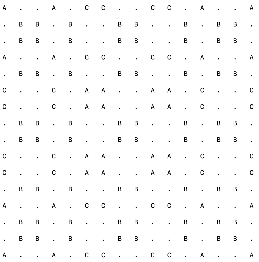
We calculate the evolution of the second order density matrices and associated variances. Matrix has the pattern shown in Figure 16, and one can observe the same pattern for , , etc. Let and be the three parameters defining . From the explicit expression in Section 19 one can show the recurrence
Writing the recurrence differently,
We immediately notice that , so the sum always remains . From we get the recurrence , leading to
Since for any we have
and
we have that
By Lemma 5 we have that is 0.5 for all . Therefore the variance of the QAOA energy for the Single Edge Graph (over random angles) for level is
| level () | 1 | 2 | 3 | 4 |
|---|---|---|---|---|
| variance | 0.0625 | 0.078125 | 0.08203125 | 0.0830078125 |