Predicting Attributes of Nodes Using Network StructureJournal: JACMVolume: 37418Journal: TISTVolume: 1111Price: 15.00DOI: 10.1145/3442390CCS: Computing methodologies Feature selectionCCS: Computing methodologies Supervised learning by classificationCCS: Information systems Nearest-neighbor search
Abstract.
In many graphs such as social networks, nodes have associated attributes representing their behavior. Predicting node attributes in such graphs is an important task with applications in many domains like recommendation systems, privacy preservation, and targeted advertisement. Attributes values can be predicted by treating each node as a data point described by attributes and employing classification/regression algorithms. However, in social networks, there is complex interdependence between node attributes and pairwise interaction. For instance, attributes of nodes are influenced by their neighbors (social influence), and neighborhoods (friendships) between nodes are established based on pairwise (dis)similarity between their attributes (social selection). In this paper, we establish that information in network topology is extremely useful in determining node attributes. In particular, we use self and cross proclivity measures (quantitative measures of how much a node attribute depends on the same and other attributes of its neighbors) to predict node attributes. We propose a feature map to represent a node with respect to a specific attribute , using all attributes of its -hop neighbors. Different classifiers are then leaned on these feature vectors to predict the value of attribute . We perform extensive experimentation on ten real-world datasets and show that the proposed method significantly outperforms known approaches in terms of prediction accuracy.
Keywords:
Attributes prediction, Data imputation, Classification, Homophily, Heterophily, Node embedding1. Introduction
In many social and collaboration networks, nodes have additional information (attributes) associated with them. Such attributed graphs are becoming increasingly common [1, 2]. The attributes could be gender or age, etc. of people in social networks [3, 4], research interests of authors in collaboration and citation networks [5], and structural or functional properties of the proteins in biological networks [6, 7].
The values of attributes reflect the characteristics, behavior, and preferences of the entities represented by the nodes. Knowledge of these attributes lead to enhanced recommendation systems [8, 9], improved community detection [10, 11, 12], and robust privacy-preserving mechanism [13, 14]. Node attributes can be utilized for graph summarization [15, 16]. They also play a key role in improving the performance of disease outbreak detection [17, 18, 19, 20, 21, 22] and early depression identification [23, 24]. In protein-protein interaction networks, attributes of proteins have been used in conjunction with network structure for protein classifications [6, 25]. Additional information about nodes (attributes values) helps design the network embeddings and graph classification algorithms efficiently [26].
In many practical scenarios, the values of all attributes are not known for all nodes, which limits the usefulness of the networks. An attribute of nodes can be inferred by considering each node as a feature vector (of dimensions equal to the number of attributes). Standard classification/regression algorithms are then employed on these feature vectors for attribute prediction [27, 28, 29]. However, this approach does not use the rich information, which is available in the form of interconnection among the nodes.
It is well known in the sociology literature that there are two kinds of interdependence between the structure of a network and attributes of nodes, namely social selection and social influence [30]. Social selection refers to the phenomenon where the similarity between nodes attributes leads to edges between them, while social influence states that edges between nodes lead to the similarity between them. Moreover, node attributes in networks exhibit the properties of homophily or heterophily [3]. Homophily (heterophily) refers to the tendency of nodes with certain values of an attribute to connect with other nodes having the same (different) values for that attribute. Figure 1 depicts an example network with one homophilic and one heterophilic attribute. The degree of homophily/heterophily is referred to as self proclivity. The notion of proclivity is extended in [3] to define cross proclivity, which is a measure of correlation among values of different attributes.
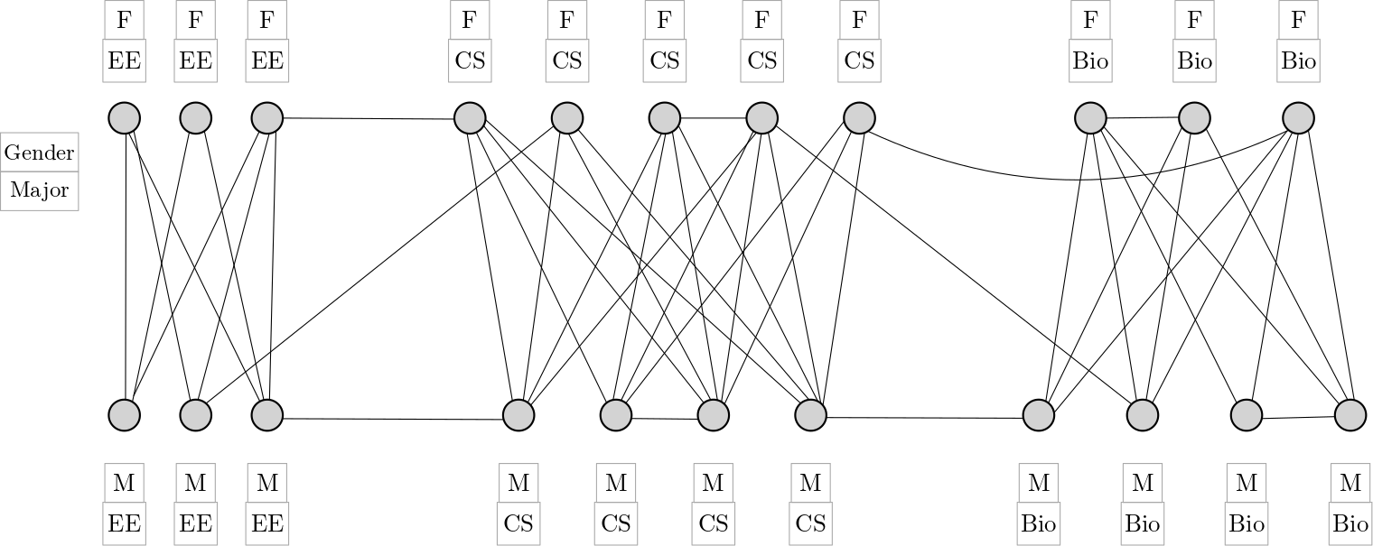
The information in network structure has been utilized for attribute prediction [31, 32, 4], node classification [33, 6, 25, 4], and other problems in graphs analysis [34, 35, 36]. Similarly, the effect of homophily has been well explored for node attribute prediction [37]. However, the cross proclivity and dependence of a node attribute on more than one attribute of its neighbors has not been utilized to its full extent.
In this paper, we propose Neighborhood based Feature Vector Representation (n-fvr) to predict node attributes in a network. We devise a feature map for nodes with respect to an attribute. These feature vectors are based on the attribute values of the node and those of the “nearby” nodes (neighbors, neighbors-of-neighbors, and so on). Standard classification/regression models are learned from the feature vectors to predict attribute values. Following are the main features of n-fvr.
- (1)
n-fvr works for both nominal and numerical attributes and is more generally applicable.
- (2)
n-fvr uses all attributes of nearby nodes to predict an attribute value for a node. Thus it captures the inherent self and cross proclivities in the network.
- (3)
Feature vector representation of nodes is based on multiple hops neighborhood capturing long term dependencies between attributes that improve predictive performance.
- (4)
Extensive evaluation of n-fvr on ten benchmark datasets demonstrates that it significantly outperforms the best-known methods for this task. n-fvr achieved up to improvement as compared to nns, up to improvement from node2vec, up to improvement from DeepWalk, up to improvement from line, up to improvement from GraRep, and up to improvement from mne in terms of accuracy.
The rest of the paper is organized as follows. In Section 2, we discuss related work to our problem. We provide detail of our feature map generation in Section 3. In Section 4, we describe the implementation details of comparisons methods and different classification/regression algorithms. Section 5 presents the results of our method and comparison. We conclude the paper in Section 6 and discuss some future directions.
2. Related Work
With increasing volume and decreasing veracity of network data with node attributes, the problem of data imputation has attracted significant attention from researchers [38, 39, 40, 41]. Both supervised [27, 29] and unsupervised [42] machine learning methods have been used to predict node attributes. These methods consider each node as a data point described by its attributes. For online social networks, additional features extracted from the contents shared by users have been used to predict node attributes. A method based on linguistic features (verbs, pronouns, articles, and prepositions) of social media content is proposed in [43] to determine users’ gender. Similarly, in [44], the model uses “likes" of people on Facebook to find binary attributes (single vs. in-relationship, smoker vs. non-smoker, etc.) of users.
These approaches, however, do not utilize the rich information in the topology of the network [3, 30, 4]. Graph clustering based methods are proposed in [45, 46] to predict characteristics of nodes based on their communities. Exploiting homophily of attributes [14, 47] uses friendship links and group information in social media to predict users’ attributes. However, the underlying assumption of having more homogeneous communities in social networks restricts the applicability as well as limits the predictive accuracy of these approaches. A two-phase (clustering-semantic similarity) approach to predict attributes values of nodes in a network is proposed in [48].
In the representation learning approach, nodes are first mapped to feature vectors (node embedding) using their attributes and network connectivity [49, 50, 41, 51]. A classifier is then learned on these vectors to predict node attributes. The DeepWalk approach in [52] employs skip-gram (a word representation model) to learn node representations in the graph. In [53], large-scale information network embedding (line) is proposed to learn representations by preserving the first- and second-order proximities of nodes. GraRep [54] uses global structural information for learning low dimensional node embedding for weighted graphs. One of the most common node embedding approaches is node2vec [55], which learns continuous feature vectors for nodes using a flexible biased random walk that can explore neighborhoods in both breadth-first search and depth-first search fashion. The latent multi-group membership graph model (lmmg)[31] summarizes the network structure, predict edges between nodes, and estimate attributes values. Several studies have proposed methods to incorporate different facets/structures of nodes into representation learning [32, 56]. These multi-facets based models aim to separately capture different characteristics of the network rather than designing single feature vector for all characteristics. In [33], an unsupervised approach called embedding propagation (em) for graph-structured data is devised. A framework, Joint Adversarial Network Embedding (JANE) is proposed in [41] to efficiently capture semantic variations in data distribution. Yang et al. [57] analyzes correlations between topological and non-topological features for a network embedding approach in which nodes, communities, and topics (attributes) are mapped into one embedding space.
The representation learning approach has yielded great success in capturing complex relationships across various disciplines such as biological networks and social media [49, 50]. In this approach, the dataset is mapped to a fixed-dimensional vector space, and machine learning methods are employed on these feature vectors for classification. In a highly successful method, these feature vectors are based on counts of various substructures in the objects. A kernel function to estimate the pairwise similarity between objects is then defined and used for classification. This approach has been used for classifying images [58], sequences [59, 60], and graphs [61, 62, 51]. In the descriptors learning approach, objects are mapped to low dimensional vectors of features extracted from objects with the goal to map similar objects closely in the Euclidean space. Many descriptors have been proposed for sequences [63, 64] electricity consumptions [65, 66] and graphs [67, 68, 69, 70, 36]. More recent but computationally expensive methods employ deep networks together with domain specific techniques for embedding nodes [33], graphs [71, 72] and texts [73, 74, 75].
3. Proposed Approach
In this section, we formulate the problem of node representation and attribute prediction and provide detail of the proposed method, Neighborhood based Feature Vector Representation (n-fvr) of nodes in attributed graphs.
3.1. Notation and Problem Formulation
Given an undirected attributed graph , where is the set of nodes, is the set of edges, , and = is the set of node attributes, an integer , and a target attribute , our goal is to predict the value of for nodes. We propose a vector representation for each vertex , based on the attributes of and values of all attributes of nodes that are ‘close by’ to . The notion of closeness is determined by the value of parameter . These vectors are then passed to a classification or regression model with the target attribute () as class label, to predict the value of for nodes.
Attributes can be nominal, ordinal or numerical. We assume all numerical attributes take discrete values (this can be achieved by appropriate discretization). Each attribute takes exactly one value from the set , where and . We assume that for every , contains a special symbol for missing value. For instance, if is the gender attribute, then , where represents missing value. We consider the attribute as a function such that . The set maps each node to a -dimensional vector, whose coordinate is . Hence, is a vector valued function given by:
| (1) |
Let be the set of neighbors of and let be the degree of . We describe the notion of nodes that are “close to" . For an integer , denote by the set of nodes that are hops away from . Formally:
| (2) |
where is the distance between node and (hop-length of the shortest path between and ). Note that and .
3.2. Aggregating attributes values of sets of nodes
Note that attributes are defined for individual nodes (see Equation (1)) and not for sets of nodes. We therefore, extend the notion of attributes to sets of nodes. For a set , we define to be the vector valued function to determine the “value" of an attribute of the set . Recall that . For a set , the function returns a dimensional real vectors, that is essentially the (discrete) distribution of values of in the set . More formally, for , the function is defined as follows:
| (3) |
where is the coordinate of the vector .
3.3. Pairwise interconnection between attributes: self and cross proclivity
To find the interconnection between two attributes and , we analyze the global connectivity structure of input graph with respect to attributes and . Recall that is the number of distinct values the attribute assumes. The information about interconnection structure between two attributes and is summarized in a matrix of size called Mixing Matrix . has a row (respectively column) corresponding to each distinct possible value of attribute (respectively . For and , the entry of counts the number of edges (in the whole graph) connecting two nodes with attribute value of to nodes with attribute value of . More precisely:
| (4) |
From construction of the mixing matrix it is clear that when values in are distributed more uniformly, then a given value of does not reveal much information about for some neighbor of . However, if the distribution of numbers in is more skewed, then knowing the value of one might be able to estimate the likelihood of a given value of for some neighbor of .
The spread of values in are quantitatively measured by the ‘divergence’ of . The divergence of a real matrix with respect to a function (an input parameter) is defined as:
| (5) |
where is a generative function, which can take values , or . The term is the sum of values in the row, is the sum of values in the column, is the sum of all entries of the matrix .
The proclivity value (self/cross) between a pair of attributes (based on ) is inversely proportional to the divergence of . A quantitative measure called “proclivity index for attributed networks" (prone) is proposed in [3]. prone value between two attributes and is defined as:
| (6) |
3.4. Construction of n-fvr
Given a target node attribute and an integer , (), n-fvr constructs the feature vector of a node with respect to the attribute . In the following we give a formal description of . For , the network structure is not considered, and is generated using only node ’s attributes. We refer to this approach as “No-Network-Structure (nns)" and define it as:
| (7) |
For , we need to consider the attributes of nodes that are at distance at most from .
3.4.1. Weight of -hop neighborhood
It is more likely that immediate neighbors reveal more information about than distant neighbors. Therefore, more importance should be given to immediate neighbors () as compared to far away neighbors (). Value of an attribute of the sets of node () is a “weighted" sum of (weighted by ), for . Here is a network specific parameter that quantifies the diminishing influence of increasingly farther neighbors on . More precisely:
| (8) |
where is as defined in (3).
3.4.2. Weight of attributes
As discussed above, attributes have varying correlation with other attributes of their neighbor. This is reflected in the construction of by giving attributes weights based on their proclivities. For , is the weighted concatenation (weight is ) of attributes values of . This is formally defined as:
| (9) |
where, represents the concatenation operation. We call the technique presented in Equation (9) as n-fvr. Also we design another approach called “nns and n-fvr" or “nn-fvr", which is simply the concatenation of the vectors generated from Equation (7) and Equation (9). The equation for nn-fvr is given as:
| (10) |
Step by step procedure of our proposed approach is given in Algorithm 1 and illustrated in Figure 2. In Algorithm 1, the For loops at line and are used to traverse the (hop length) and all attributes of nodes respectively. Line aggregates the attributes values of neighbors (see Equation (2) and (3)) to generate a single feature vector with respect to an attribute and multiply attribute weight (see Equation (6)) and hops weight with the feature vectors. Line concatenate the feature vectors of attributes and generate a separate feature vector for each value of . These vectors are then aggregated in line to make a single feature vector for all levels of . The feature vector is then normalized by dividing it with the degree of () in line to generate final feature vector representation for with respect to attribute , for which missing value is being predicted.
3.5. Runtime Analysis of prone and n-fvr
For a graph with and , the mixing matrix (given in Equation (4)) can be populated in one linear scan over the edges in . The divergence (given in Equation (5)) of can be computed in steps, where and are the number of levels of attributes and , respectively. Thus prone (given in Equation (6)) can be computed in time. Note that (the number of edges in a graph is typically much larger than the number of levels of an attribute). Moreover, the prone value needs to be computed for each target attribute only once.
In case of n-fvr, feature vector for an attribute of node can be learned in (when ). For all nodes, this runtime is , where is the number of edges in the whole graph. For , the runtime of a node is . For , the runtime of a node is and so on.

4. Experimental Setup
In this section, we describe the experimental setup, details of the ten benchmark datasets, comparison algorithms, the classification models we employed, and evaluation metrics.
4.1. Datasets Description
We use eight datasets from a collection of “Facebook100" datasets, which are friendship networks of US universities [76]. These datasets include “Caltech", “Rice", “American", “UChicago", “Mississippi", “Temple", “Haverford", and “UNC". In each of these datasets, a node represents a user, and an edge between two nodes represents friendship. Each node has four associated categorical attributes, (i) status (faculty/student/etc.), (ii) gender, (iii) dormitory, and (iv) enrolled year.
The next dataset is also a friendship network that is a subgraph of Pokec [77], a popular Slovak online social network. Each node in this graph has three associated attributes, (i) status (public/private), (ii) gender, and (iii) age.
The last dataset is 4area, a bibliographic network extracted from dblp [78]. A node in this dataset represents an author and edges show co-author relationships. Each node has four attributes corresponding to four domains of computer science namely (i) database (db), (ii) data mining (dm), (iii) machine learning (ml), and (iv) information retrieval (ir). Attributes values are the fraction of research papers published by the authors in these areas. Note that attributes values in this dataset are continuous. For classification, we discretize attributes by binning into bins. However, for regression, we used the original continuous values. The statistics of datasets and training splits are presented in Table 1. The train-test split is as in the literature, to ensure a fair comparison.
| Dataset | Name | No. of Nodes | No. of Edges | No. of Attributes | Train (%) |
|---|---|---|---|---|---|
| Facebook100 | Caltech | 70 | |||
| Haverford | 1,5,9 | ||||
| Rice | 70 | ||||
| American | 70 | ||||
| UChicago | 1,5,9 | ||||
| Mississippi | 1,5,9 | ||||
| Temple | 1,5,9 | ||||
| UNC | 80 | ||||
| Slovak Social Network | Pokec | 70 | |||
| Bibliography Network | 4area | 70 |
4.2. Comparison Algorithms
We compare our approach with several methods that have been reported to have the best results on the corresponding datasets. These methods are the following:
- (1)
nns: In this approach, network structure is not considered. The feature vector is generated using only the attributes of nodes (see Equation (7)).
- (2)
wvrn [79] (2003): It is a weighted relational classifier that estimates attribute value of a node using the weighted mean of the same attribute of ’s neighbors. Since the graphs of the datasets are unweighted, we use similarity values to assign weights to the neighboring nodes. These similarity values are computed using Euclidean distance between the feature vector of node and its neighbors.
- (3)
lmmg [31] (2012): It is a node representation model, which is based upon the idea of Multiplicative Attribute Graph (MAG) Mode. In this approach, each node can belong to multiple groups, and the occurrence of each node feature is determined by a logistic model based on the group memberships of the given node.
- (4)
DeepWalk [52] (2014): It is a representation model, which works for the unweighted graphs. The random walk method is used to translate graph structure into linear sequences. The skip-gram model with hierarchical softmax is used as the loss function. The code for DeepWalk is available online11 1 https://github.com/data-science-lab/data-science-lab.github.io/wiki/DeepWalk.
- (5)
line [53] (2015): It is a graph embedding approach, which preserves both local and global network structures and works for undirected, directed, and weighted graphs. It defines a loss function based on -step and -step relational information between nodes and combine them to get the final feature vector. The code for line is available online22 2 https://github.com/tangjianpku/LINE.
- (6)
GraRep [55] (2015): It is a node representation model for weighted graphs. This model incorporates both local and global structural information of the graph to learn the feature vector representations. The code for Grarep is available online33 3 https://github.com/benedekrozemberczki/GraRep.
- (7)
slr [37] (2016): It is an integrative probabilistic model, which is used to capture the statistical correlations (homophily effect) among attributes. It uses the triangular motif representation of the network for improved scalability and predictive performance.
- (8)
node2vec [54] (2016): It generalizes the DeepWalk method with the combination of BFS and DFS random walks. This method considers both network structure and graph homophily. The code for node2vec is available online44 4 https://snap.stanford.edu/node2vec/.
- (9)
majority [33] (2017): The majority approach takes the most frequently occurring attribute values from the neighboring nodes in the training set and assigns that value to the attributes of nodes in the test set.
- (10)
mne [32] (2018): This method captures multiple structures (facets) of the network by learning multiple embeddings simultaneously. It uses the Hilbert Schmidt Independence Criterion (HSIC) as a diversity constraint.
4.3. Prediction Models and Hyperparameters for n-fvr and nn-fvr
To evaluate the goodness of the proposed approach, we use five standard classification/regression models. These include -nearest neighbors (knn), naïve bayes (nb), decision tree (dt), support vector machine (svm), and linear regression (lr).
The hyperparameters of the feature map, , and and those of each model are set using standard validation set approach. Once these hyperparameters are tuned, unless otherwise mentioned, they remain same for all the experiments on all the datasets. The selected parameters are following:
- •
Changing the value of for knn can greatly affect the predictive performance. We performed multiple experiments and empirically set . This value remains the same across all datasets with the exception for Haverford, UChicago, Mississippi, and Temple datasets. For these datasets, the value of varies with respect to the attribute and size of training data. This was deemed necessary because of the different training splits (as opted in the baseline study [32]). Values of for these datasets are given separately along with the results (see Table 7). Figure 3 shows the effect of changing on different attributes of Caltech dataset. Similar behavior is observed on other datasets.
Figure 3. Effect of on accuracy using knn algorithm on different attributes of caltech dataset utilizing n-fvr. - •
We only have one parameter for nb that is smoothing value, which is set to .
- •
The metric for root and attribute selection for dt is performed by utilizing “gini index" value.
- •
The kernel used for svm is “linear" while classification type used is “C-classification" with value of “C" is taken as .
- •
We implement linear regression using “qr matrix decomposition" instead of “svd decomposition" due to its computational efficiency.
- •
For each value of , we use different weight so that equal importance is not given to immediate and far-away neighbors. We perform multiple experiments to select the value for from a range of . We empirically decide the value for and for .
4.4. Evaluation Metrics and Implementation Details
We use standard metrics from literature to evaluate the performance of our method. These metrics include accuracy, F1-measure, Mean Absolute Error (mae), Root Mean Squared Error (rmse), Mean Squared Error (mse), and .
All experiments were carried out on a machine with an Intel(R) Core i CPU processor at GHz and GB of DDR memory. Our code is implemented in R (for feature vector generation and classification algorithms) and Weka (for linear regression). The code is made publicly available for reproducibility and further experimentation 55 5 https://github.com/sarwanpasha/Attriubute-Prediction-Code.
5. Results and Comparisons
This section presents the empirical evaluation of our model and its comparison with several baseline methods. First, we present the heat map of the prone values for each pair of attributes of all datasets.
5.1. prone values ()
We present the prone values between each pair of attributes for all datasets in Figure 4. The diagonal entries of these tables show the self-proclivity values for the corresponding attributes. The off-diagonal values show the cross-proclivity values between the corresponding pairs of attributes. These results are computed by taking value of generative function as in Equation (5). Identical trend is observed in case of and .


As can be seen in Figure 4, dormitory attribute has the highest self proclivity in case of Caltech and Rice datasets (i.e., people belonging to the same dormitory tend to be friends). It essentially means that given Alice and Bob are friends, if we know the dormitory value for Alice, then we can predict the dormitory value of Bob. However, gender shows very small self proclivity, therefore, the same cannot be said for it. This behavior is also observed for other facebook100 datasets. Interestingly, in the case of 4area dataset, many pairs of attributes pose high cross proclivity. This means that we can predict any attribute of 4area dataset using any other attribute of neighbors with high accuracy.
5.2. Comparison with the Baseline Methods
As mentioned earlier, we perform experiments by considering hop neighborhood. We first focus the discussion for .
The results for American and Rice datasets are presented in Table 2. As can be seen, our methods significantly outperform the baselines (highest accuracy values are shown in boldface). However, the overall performance varies with respect to predicted attribute, classifier, and the fvr type used. The dt classifier on nn-fvr shows better performance than other classifiers in case of “status" and “gender" attributes of both datasets. However, the highest accuracy is achieved with svm for “dormitory" attribute. The knn algorithm with n-fvr show highest performance when predicting “year" attribute of both datasets. However, these analyses do not help us to draw strong conclusions in favor of a particular setting of our experimentation. Hence, the results of one classifier on a particular attribute of a dataset cannot be generalized to all attributes. We also show the percentage improvement from nns to the best performing variation of the experiments utilizing n-fvr and nn-fvr. The highest gain in performance is observed for predicting “dormitory" attribute using nn-fvr in case of American dataset () and n-fvr in case of rice dataset ().
| Method | American | Rice | |||||||
| Status | Gender | Dormitory | Year | Status | Gender | Dormitory | Year | ||
| wvrn | 85.49 | 56.67 | 67.06 | 71.71 | 86.12 | 54.80 | 84.46 | 74.72 | |
| majority | 85.43 | 56.84 | 67.11 | 70.99 | 85.71 | 55 | 83.50 | 73.64 | |
| nns | 79.59 | 59.70 | 16.93 | 38.96 | 70.33 | 57.22 | 10.65 | 29.79 | |
| n-fvr knn | 88.56 | 62.86 | 70.66 | 83.45 | 89.07 | 62.02 | 94.29 | 84.91 | |
| n-fvr nb | 80.16 | 62.86 | 36.79 | 48.63 | 76.28 | 52.70 | 78.59 | 50.27 | |
| n-fvr dt | 88.51 | 62.86 | 54.23 | 81.55 | 87.85 | 52.70 | 92.24 | 81.71 | |
| n-fvr svm | 80.84 | 62.86 | 43.44 | 81.25 | 84.59 | 52.70 | 94.29 | 77.33 | |
| nn-fvr knn | 80.01 | 59.92 | 21.57 | 61.80 | 75.55 | 57.22 | 45.70 | 47.80 | |
| nn-fvr nb | 76.36 | 61.23 | 79.06 | 50.54 | 80.16 | 60.80 | 36.79 | 48.87 | |
| nn-fvr dt | 91.60 | 64.89 | 92.24 | 82.54 | 90.24 | 67.68 | 55.14 | 83.51 | |
| nn-fvr svm | 85 | 52.52 | 93.55 | 78.88 | 81.41 | 62.86 | 43.85 | 81.43 | |
| Improvement from nns to n-fvr (%) | 8.97 | 3.16 | 53.73 | 44.49 | 18.74 | 4.8 | 83.64 | 55.12 | |
| Improvement from nns to nn-fvr (%) | 10.65 | 5.19 | 76.62 | 43.58 | 19.91 | 10.46 | 44.49 | 53.72 | |
The results for Pokec and 4area (after dividing attributes values into bins) datasets are shown in Table 3. In regards to Pokec dataset, the dt classifier with n-fvr and nn-fvr shows highest performance for “public" attribute. In case of “gender" attribute, knn with n-fvr performs better. An interesting behavior is observed in case of “age" attribute, where wvrn outperform both n-fvr and nn-fvr by a small margin. Most interesting results are achieved on 4area dataset, on which the svm classifier with nn-fvr outperforms all other approaches for all the attributes. Overall, nn-fvr perform better than nns as evident from the mentioned performance gains. Note that for 4area dataset, every model and classifier achieve accuracy greater than . This is because of the fact that there is a high self/cross proclivity among attributes of 4area dataset (see Figure 4). It is observed that high self/cross proclivity enables all models to efficiently learn the patterns in the data, consequently leading to higher predictive performance. Therefore, we only observed minor performance gain for nn-fvr model (and negative gain for n-fvr model). However, since high proclivity is usually not observed in real-world scenarios (as can be seen in Figure 4), it can be concluded that the proposed model is more applicable in real-world settings.
| Method | Pokec | 4area | ||||||
|---|---|---|---|---|---|---|---|---|
| Public | Gender | Age | db | dm | ir | ml | ||
| wvrn | 46.2 | 42.2 | 25.6 | 90.40 | 88.94 | 88.97 | 89.95 | |
| majority | 49.1 | 40.5 | 25.2 | 90.17 | 88.84 | 88.57 | 89.68 | |
| nns | 52.33 | 61.33 | 16.74 | 97.60 | 97.50 | 97.30 | 97.90 | |
| n-fvr knn | 87 | 66 | 23.78 | 92.83 | 92.26 | 92.01 | 92.40 | |
| n-fvr nb | 86.33 | 60.66 | 18.50 | 88.71 | 87.21 | 87.65 | 88.05 | |
| n-fvr dt | 87.66 | 61 | 21.58 | 92.45 | 92.59 | 91.48 | 92.93 | |
| n-fvr svm | 81 | 57 | 14.09 | 92.64 | 92.47 | 91.80 | 93.11 | |
| nn-fvr knn | 80.66 | 64.33 | 25.11 | 96.30 | 95.52 | 95.46 | 96.18 | |
| nn-fvr nb | 86.33 | 60.66 | 18.94 | 90.04 | 89.31 | 89.02 | 90.88 | |
| nn-fvr dt | 87.66 | 65.33 | 18.50 | 95.80 | 95.49 | 95.06 | 95.69 | |
| nn-fvr svm | 82.66 | 57 | 16.74 | 97.61 | 97.59 | 97.46 | 97.92 | |
| Improvement from nns to n-fvr (%) | 35.33 | 4.67 | 7.04 | -4.77 | -4.91 | -5.29 | -4.79 | |
| Improvement from nns to nn-fvr (%) | 35.33 | 4 | 8.37 | 0.01 | 0.09 | 0.16 | 0.02 | |
| Method | Caltech | |||
|---|---|---|---|---|
| Status | Gender | Dormitory | Year | |
| wvrn | 80.88 | 60.46 | 74.25 | 67.23 |
| lmmg | 77 | _ | _ | _ |
| majority | 79.97 | 59.03 | 72.82 | 65.14 |
| nns | 69.69 | 65.40 | 18.33 | 31.97 |
| n-fvr knn | 87.01 | 62.08 | 88.88 | 80.20 |
| n-fvr nb | 75.75 | 64.45 | 72.22 | 51.26 |
| n-fvr dt | 86.58 | 64.45 | 82.22 | 74.61 |
| n-fvr svm | 69.69 | 68.72 | 72.77 | 28.42 |
| nn-fvr knn | 70.99 | 65.40 | 28.33 | 36.04 |
| nn-fvr nb | 75.75 | 64.45 | 72.22 | 51.77 |
| nn-fvr dt | 92.20 | 64.45 | 82.22 | 78.17 |
| nn-fvr svm | 71.42 | 68.72 | 54.44 | 38.57 |
| Improvement from nns to n-fvr (%) | 17.32 | 3.32 | 70.55 | 48.23 |
| Improvement from nns to nn-fvr (%) | 22.51 | 3.32 | 63.89 | 46.20 |
In Table 4, we show the results for Caltech dataset. It is evident from the results that our method significantly outperforms existing approaches. The dt with nn-fvr significantly performs better than other approaches for prediction of status attribute. In the case of gender attribute, svm shows equal performance for both n-fvr and nn-fvr based approaches. While for other two attributes, knn classifier on n-fvr yields maximum accuracy. As compared to baseline models, the proposed approach yields noticeable performance improvements. Note that we took the accuracy results of the lmmg approach from the original study [31], where the authors has reported the results for one attribute only (other attributes are left empty in Table 4).
Results in Table 5 show the F1-score of our method and other baseline approaches on UNC dataset. We report -score to make fair comparison with the results given in [37] on the respective dataset. We can see in the results that our method significantly outperforms all baseline approaches. The F1-score of the slr and svd++ approaches were mentioned for only one attribute “status" in the original study (other attributes are left empty in Table 5). As far as attribute specific performance is concerned, dt with nn-fvr shows highest F1-score while predicting “status" and “dormitory" attributes. Similarly, svm based on n-fvr yields maximum performance while predicting the “gender" and “year" attributes.
| Method | UNC | |||
|---|---|---|---|---|
| Status | Gender | Dormitory | Year | |
| wvrn | 51.57 | 40.12 | 29.46 | 48.16 |
| slr-e | 43 | _ | _ | _ |
| slr-m | 41 | _ | _ | _ |
| svd++ | 57 | _ | _ | _ |
| majority | 49.87 | 39.22 | 26.17 | 45.40 |
| nns | 40.20 | 57.77 | 7.53 | 33.48 |
| n-fvr knn | 69.14 | 54.19 | 24.30 | 58.58 |
| n-fvr nb | 44.77 | 53.59 | 8.49 | 24.08 |
| n-fvr dt | 67.74 | 57.96 | 35.07 | 68.74 |
| n-fvr svm | 72.18 | 73.34 | 19.47 | 76.39 |
| nn-fvr knn | 38.65 | 56.81 | 7.80 | 41.73 |
| nn-fvr nb | 44.77 | 53.62 | 8.49 | 24.16 |
| nn-fvr dt | 74.56 | 62.83 | 38.99 | 71.28 |
| nn-fvr svm | 73.78 | 43.07 | 9.69 | 73.70 |
| Improvement from nns to n-fvr (%) | 31.98 | 15.57 | 27.54 | 42.91 |
| Improvement from nns to nn-fvr (%) | 34.36 | 5.06 | 31.46 | 40.22 |
Recall that actual attributes values of 4area dataset are continuous. Now we present the results on continuous values and compare them with nns. Table 6 show the mae, rmse, , and mse values for attributes of area dataset. We apply linear regression on the feature vectors generated using n-fvr and nn-fvr approaches. Our method nn-fvr show comparable results with nns. We do not compare our methods with wvrn and majority because they do not work for continuous dataset.
| Method | 4area | |||||||||||||||
|---|---|---|---|---|---|---|---|---|---|---|---|---|---|---|---|---|
| db | dm | ir | ml | |||||||||||||
| mae | rmse | mse | mae | rmse | mse | mae | rmse | mse | mae | rmse | mse | |||||
| nns | 0 | 0 | 1 | 0 | 0 | 0 | 1 | 0 | 0 | 0 | 1 | 0 | 0 | 0 | 1 | 0 |
| n-fvr | 0.07 | 0.14 | 0.87 | 0.02 | 0.07 | 0.15 | 0.79 | 0.02 | 0.08 | 0.16 | 0.81 | 0.02 | 0.07 | 0.15 | 0.89 | 0.02 |
| nn-fvr | 0 | 0 | 1 | 0 | 0 | 0 | 1 | 0 | 0 | 0 | 1 | 0 | 0 | 0 | 1 | 0 |
To the best of our knowledge, Multi-Facet Network Embedding (mne) (2018) is the current best solution for our problem. mne has made comparisons with several generic techniques like DeepWalk [52] (2014), line [53] (2015), GraRep [55] (2015), and node2vec [54] (2016). Yang et. al. in [32] already demonstrated (both theoretically and empirically) that mne outperformed those generic techniques in accuracy. Therefore, outperforming mne implies that our algorithm also outperforms the generic techniques. Thus, rather than separately comparing our model with each generic approach, we use the results reported in [32] to make the comparisons. Results in Table 7 show the comparison of our method with mne, DeepWalk, line, GraRep, and node2vec. Since the authors did not use “status" attribute in their study in [32], we also omit this particular attribute in our experiments. To make a fair comparison, we selected the same percentage of the training set (, , and ) as given in [32]. Note that contrary to previous results, we only use knn for this particular comparison (due to its higher performance). Optimum values of for knn are selected empirically for each dataset, attribute, and training percentage. This was deemed necessary because of the unique setting of train split percentages. It is evident from the results given in Table 7 that our approach (n-fvr) outperform all other baselines in most of the cases (up to % improvement from mne) with exception in a few cases.
| UChicago | Temple | |||||||||||||||||
| Techniques | Gender | Year | Dormitory | Gender | Year | Dormitory | ||||||||||||
| DeepWalk | 50.1 | 52.3 | 55.9 | 55.6 | 59.1 | 63.8 | 20.2 | 35.7 | 47.4 | 50.1 | 55.5 | 58.2 | 51.1 | 55.7 | 60.3 | 21.4 | 31.8 | 36.1 |
| line | 52.1 | 54.1 | 56.9 | 61 | 61.9 | 65.2 | 21.1 | 43.5 | 50.1 | 52.9 | 57.9 | 58.5 | 56.3 | 66.9 | 69.6 | 25.4 | 32.7 | 38.2 |
| GraRep | 47.7 | 48.5 | 50.1 | 50.5 | 55.3 | 59.9 | 18.6 | 30.3 | 40 | 45.6 | 49 | 55 | 50.3 | 57.2 | 65.1 | 21.7 | 29.6 | 31.5 |
| node2vec | 51.3 | 53.5 | 55.2 | 60.2 | 61.2 | 64.1 | 22.1 | 39.8 | 49.7 | 51 | 54.8 | 57.9 | 52.8 | 55.3 | 64.2 | 20.2 | 29.8 | 38.1 |
| mne | 54.5 | 57.7 | 59.7 | 58.1 | 65.9 | 67.7 | 24.8 | 48.2 | 54.4 | 55.9 | 61.4 | 62.9 | 61.5 | 69.9 | 72.7 | 30.1 | 36.1 | 41.9 |
| n-fvr | 55.8 | 56.6 | 56.7 | 70.7 | 74.3 | 75 | 25.8 | 46.1 | 54.1 | 57.3 | 57.5 | 58.3 | 69.4 | 70.3 | 70.6 | 37.8 | 45.4 | 48.4 |
| nn-fvr | 52.3 | 52.4 | 52.4 | 52.5 | 71.1 | 71 | 8 | 16.6 | 22.1 | 57 | 57.1 | 57.1 | 57.3 | 67.8 | 68 | 21.6 | 29.2 | 29.4 |
| Value of | 12 | 97 | 3 | 4 | 4 | 17 | 1 | 1 | 1 | 89 | 45 | 24 | 26 | 18 | 25 | 6 | 9 | 10 |
| Improvement from mne (%) | 1.3 | -1.1 | -3 | 12.6 | 8.4 | 7.3 | 1 | -2.1 | -0.3 | 1.4 | -3.9 | -4.6 | 7.9 | 0.4 | -2.1 | 7.7 | 9.3 | 6.5 |
| Haverford | Mississippi | |||||||||||||||||
| Techniques | Gender | Year | Dormitory | Gender | Year | Dormitory | ||||||||||||
| DeepWalk | 50.6 | 53.5 | 57.3 | 61.4 | 76.7 | 81.1 | 29 | 37.4 | 43.9 | 53.1 | 60.4 | 60.9 | 46.5 | 55.3 | 61.6 | 32.5 | 44.1 | 48.3 |
| line | 50.1 | 51.6 | 52.9 | 59.1 | 76.1 | 80.5 | 27.9 | 36.6 | 41.5 | 55.3 | 62.7 | 64.7 | 48.6 | 58.9 | 63.2 | 34.2 | 48.9 | 53.4 |
| GraRep | 48.8 | 51.1 | 51.9 | 57.4 | 72.1 | 77.5 | 29 | 39.8 | 42.9 | 44.6 | 48 | 52.9 | 42.7 | 48.3 | 49.2 | 32.5 | 45.9 | 52.1 |
| node2vec | 51.3 | 57.1 | 57.1 | 57.6 | 75.6 | 79.1 | 29.2 | 41.4 | 43.8 | 52.6 | 59.8 | 59.8 | 47.2 | 56.8 | 60.1 | 31.3 | 39.5 | 44.1 |
| mne | 54.2 | 59.6 | 62.0 | 66.9 | 81.3 | 84.4 | 33 | 45.7 | 47.6 | 58.9 | 65.9 | 68 | 53.3 | 59.4 | 63.8 | 38.7 | 53.7 | 56.7 |
| n-fvr | 63.8 | 64.2 | 63.9 | 78.9 | 81.9 | 83.4 | 38.3 | 41.6 | 47.5 | 63.2 | 67.1 | 68.7 | 68.7 | 68.4 | 68.8 | 43.9 | 56.6 | 60.8 |
| nn-fvr | 54.3 | 55.9 | 57.3 | 34.3 | 54 | 63.9 | 37.1 | 38.3 | 39.4 | 55 | 58 | 60.4 | 56.3 | 67.9 | 67.7 | 15.2 | 27.9 | 30 |
| Value of | 7 | 29 | 48 | 1 | 3 | 6 | 10 | 9 | 7 | 1 | 4 | 6 | 12 | 38 | 42 | 4 | 5 | 14 |
| Improvement from mne (%) | 9.6 | 4.6 | 1.9 | 12 | 0.6 | -1 | 5.3 | -4.1 | -0.1 | 4.3 | 1.2 | 0.7 | 15.4 | 9 | 5 | 5.2 | 2.9 | 4.1 |
5.3. Effect of on predictive performance
Next, we investigate the effect of hop length on accuracy. Results in Figure 5 show the accuracy with increasing value of for Caltech dataset. The results show a general trend of performance improvement (in most cases) when going from to , with a few exceptions. However, going from to , the performance gains are minimal. Turning now to discussion about the specific classifiers, the performance of svm tend to increase for . On the other hand, on average, the performance of nb classifier tends to increase (except for gender attribute) with the increase in the value of . The performance of knn does not have any noticeable effect in most cases. These results also vary with datasets. Additional experiments reveal that going beyond is dataset and attribute specific decision. No generic conclusion can be drawn with respect to these choices. For example, in Caltech dataset, it is evident from Figure 5 that there is no significant gain in the accuracy of status, dormitory, and year attributes in case of knn classifier for increasing value of . However, we can observe slight improvement in accuracy of gender attribute in case of (using n-fvr). From the results in Figure 5, we can conclude that knowing the attributes values of neighbors of a node that are multiple hops away (i.e., ) provides no (or minimal) additional information for predicting the attributes of node (immediate neighbors have more influence on ). However, this conclusion does not hold for svm classifier, where we record significant performance boost for . We observe similar behavior for other datasets as well. Results of other datasets for increasing value of are shown in appendix A.
5.4. Effect of Self and Cross Proclivity
Experimental results reveal that higher correlation amongst attributes results in higher predictive performance of the classifiers. The most noticeable effect of this phenomenon can be observed in case of 4area dataset, which has higher self/cross proclivity (see Figure 4). On this dataset all classifiers achieve accuracy greater than (see Table 3). We observed that higher self or cross proclivity alone does not yield increased accuracy. Effect of combining both proclivity measures can be observed for the datasets with low self/cross proclivity values among attributes. In this case, lower performance gains are achieved by the baseline methods including nns. However, since the proposed method is taking both self and cross proclivity into account, higher accuracy. This accuracy vs. correlation behavior leads us to conclude that in a given dataset, if attributes show a high correlation amongst themselves (high self/cross proclivity), most predictive methods are very likely to predict attributes with higher accuracy and vice versa.
5.5. Limitations
Analysis of results reveals that when there is a high proclivity (self/cross) among the attributes, the proposed method does not perform significantly better than nns. This is evident from the results of 4area dataset (see Table 3). Even in this scenario, our method is competitive in majority of cases, but it does not significantly outperform existing methods. However, in majority of the real-world scenarios, high proclivity is not prevalent (see Figure 4). Secondly, we observe that as the number of unique values in attributes increases, the accuracy of underlying classifiers tends to decrease. This behavior is observed for all methods.
6. Conclusion and Future Work
We propose a method to generate feature vectors for the nodes based on other attributes values of that node and its neighbors. These feature vectors then input to standard machine learning algorithms to predict attributes. Our approach efficiently predicts attributes with high accuracy and outperforms existing methods. Through extensive experimentation on several benchmark datasets, we also show that our approach works for different types of datasets, highlighting the proposed approach’s generalizability. One possible future direction is to combine statistical-based learning algorithms with the proposed approach to design an ensemble technique to construct richer feature vector representations for node attributes. Another possible extension is to use the proposed method to design feature vectors for the nodes or graphs in general that can then be used for node or graph classification. An interesting future research direction is to make the weight parameter a model parameter and learn it from the data. Similarly, more complex models’ influence of neighborhoods on nodes’ attributes is another possible extension of this work.
References
- [1] P. Goyal and E. Ferrara. Graph embedding techniques, applications, and performance: A survey. Knowledge-Based Systems, 151:78–94, 2018.
- [2] Z. Meng and H. Shen. Dissimilarity-constrained node attribute coverage diversification for novelty-enhanced top-k search in large attributed networks. Knowledge-Based Systems, 150:85–94, 2018.
- [3] R. Rabbany, D. Eswaran, A. Dubrawski, and C. Faloutsos. Beyond assortativity: Proclivity index for attributed networks. In Pacific-Asia Conf. on Knowledge Discovery and Data Mining (PAKDD), pages 225–237, 2017.
- [4] L. Liao, X. He, H. Zhang, and T. Chua. Attributed social network embedding. IEEE Transactions on Knowledge and Data Engineering, 30(12):2257–2270, 2018.
- [5] W. Ye, L. Zhou, X. Sun, C. Plant, and C. Böhm. Attributed graph clustering with unimodal normalized cut. In Joint European Conf. on Machine Learning and Knowledge Discovery in Databases, pages 601–616, 2017.
- [6] W. Hamilton, Z. Ying, and J. Leskovec. Inductive representation learning on large graphs. In Advances in Neural Information Processing Systems (NeurIPS), pages 1024–1034, 2017.
- [7] I. Kovács, K. Luck, K. Spirohn, Y. Wang, C. Pollis, S. Schlabach, W. Bian, D. Kim, N. Kishore, T. Hao, M. Calderwood, M. Vidal, and A. Barabasi. Network-based prediction of protein interactions. Nature communications, 10(1):1–8, 2019.
- [8] Z. Che, S. Purushotham, K. Cho, D. Sontag, and Y. Liu. Recurrent neural networks for multivariate time series with missing values. Scientific Reports, 8(1):1–12, 2018.
- [9] R. Lopes, R. Assunção, and R. Santos. Graph-based recommendation meets bayes and similarity measures. Trans. on Intelligent Systems and Technology (TIST), 11(1):1–26, 2019.
- [10] H. Sun, R. Huang, X. Jia, L. He, S. Miaomiao, P. Wang, Z. Sun, and J. Huang. Community search for multiple nodes on attribute graphs. Knowledge-Based Systems, page 105393, 2019.
- [11] J. Yang, J. McAuley, and J. Leskovec. Community detection in networks with node attributes. In Intern. Conf. on Data Mining (ICDM), pages 1151–1156, 2013.
- [12] S. Pool, F. Bonchi, and M. Leeuwen. Description-driven community detection. Trans. on Intelligent Systems and Technology (TIST), 5(2):1–28, 2014.
- [13] J. Soria-Comas and J. Domingo-Ferrer. Differentially private data publishing via optimal univariate microaggregation and record perturbation. Knowledge-Based Systems, 153:78–90, 2018.
- [14] E. Zheleva and L. Getoor. To join or not to join: the illusion of privacy in social networks with mixed public and private user profiles. In Intern. Conf. on World Wide Web (WWW), pages 531–540, 2009.
- [15] Y. Wu, Z. Zhong, W. Xiong, and N. Jing. Graph summarization for attributed graphs. In International Conference on Information Science, Electronics and Electrical Engineering, volume 1, pages 503–507, 2014.
- [16] M. Beg, M. Ahmad, A. Zaman, and I. Khan. Scalable approximation algorithm for graph summarization. In Advances in Knowledge Discovery and Data Mining (PAKDD), pages 502–514, 2018.
- [17] S. Cook, C. Conrad, A. Fowlkes, and M. Mohebbi. Assessing google flu trends performance in the united states during the 2009 influenza virus a (h1n1) pandemic. PloS One, 6(8):1–8, 2011.
- [18] S. Abbas, J. Tariq, A. Zaman, and I. Khan. Sampling based efficient algorithm to estimate the spectral radius of large graphs. In IEEE International Conference on Distributed Computing Systems Workshops, ICDCSW, pages 175–180, 2017.
- [19] M. Ahmad, J. Tariq, M. Farhan, M. Shabbir, and I. Khan. Spectral methods for immunization of large networks. In 14th Australasian Data Mining Conference (AusDM), pages 137–145, 2016.
- [20] M. Ahmad, J. Tariq, M. Shabbir, and I. Khan. Spectral methods for immunization of large networks. Australasian Journal of Information Systems, 21, 2017.
- [21] J. Tariq, M. Ahmad, I. Khan, and M. Shabbir. Scalable approximation algorithm for network immunization. In 21st Pacific Asia Conference on Information Systems, PACIS, page 200, 2017.
- [22] M. Ahmad, S. Ali, J. Tariq, I. Khan, M. Shabbir, and A. Zaman. Combinatorial trace method for network immunization. Information Sciences, 519:215 – 228, 2020.
- [23] M. Choudhury, S. Counts, E. Horvitz, and A. Hoff. Characterizing and predicting postpartum depression from shared facebook data. In Conf. on Computer Supported Cooperative Work & Social Computing (CSCW), pages 626–638, 2014.
- [24] G. Colombo, P. Burnap, A. Hodorog, and J. Scourfield. Analysing the connectivity and communication of suicidal users on twitter. Computer Communications, 73:291–300, 2016.
- [25] Y. Hou, H. Chen, C. Li, J. Cheng, and M. Yang. A representation learning framework for property graphs. In Intern. Conf. on Knowledge Discovery & Data Mining (SIGKDD), pages 65–73, 2019.
- [26] C. Li, S. Wang, D. Yang, S. Philip, Y. Liang, and Z. Li. Adversarial learning for multi-view network embedding on incomplete graphs. Knowledge-Based Systems, 180:91–103, 2019.
- [27] S. Alam, G. Dobbie, and X. Sun. Improving imputation accuracy in ordinal data using classification. In Intern. Conf. on Intelligent Systems Design and Applications (ISDA), pages 45–56, 2016.
- [28] J. Jia and N. Gong. Attriguard: A practical defense against attribute inference attacks via adversarial machine learning. In USENIX Security Symposium, pages 513–529, 2018.
- [29] X. Su, R. Greiner, T. Khoshgoftaar, and A. Napolitano. Using classifier-based nominal imputation to improve machine learning. In Advances in Knowledge Discovery and Data Mining (PAKDD), pages 124–135, 2011.
- [30] K. Lewis, M. Gonzalez, and J. Kaufman. Social selection and peer influence in an online social network. Proceedings of the National Academy of Sciences (PNAS), 109(1):68–72, 2012.
- [31] M. Kim and J. Leskovec. Latent multi-group membership graph model. In Intern. Conf. on Machine Learning (ICML), pages 1–10, 2012.
- [32] L. Yang, Y. Guo, and X. Cao. Multi-facet network embedding: Beyond the general solution of detection and representation. In AAAI Conf. on Artificial Intelligence, pages 499–506, 2018.
- [33] A. Duran and M. Niepert. Learning graph representations with embedding propagation. In Advances in Neural Information Processing Systems (NeurIPS), pages 5119–5130, 2017.
- [34] T. Khot, S. Natarajan, K. Kersting, and J. Shavlik. Gradient-based boosting for statistical relational learning: the markov logic network and missing data cases. Machine Learning, 100(1):75–100, 2015.
- [35] J. Neville and D. Jensen. Relational dependency networks. Jour. of Machine Learning Research (JMLR), 8:653–692, 2007.
- [36] Z.R Hassan, M. Shabbir, I. Khan, and W. Abbas. Estimating descriptors for large graphs. In Advances in Knowledge Discovery and Data Mining (PAKDD), pages 779–791, 2020.
- [37] L. Liao, Q. Ho, J. Jiang, and E. Lim. Slr: A scalable latent role model for attribute completion and tie prediction in social networks. In Intern. Conf. on Data Engineering (ICDE), pages 1062–1073, 2016.
- [38] S. Bartunov, A. Korshunov, S. Park, W. Ryu, and H. Lee. Joint link-attribute user identity resolution in online social networks. In Intern. Conf. on Knowledge Discovery and Data Mining (SIGKDD), pages 1–9, 2012.
- [39] N. Gong, A. Talwalkar, L. Mackey, L. Huang, E. Shin, E. Stefanov, E. Shi, and D. Song. Joint link prediction and attribute inference using a social-attribute network. Trans. on Intelligent Systems and Technology (TIST), 5(2):1–20, 2014.
- [40] B. Horne, J. Nørregaard, and S. Adali. Robust fake news detection over time and attack. Trans. on Intelligent Systems and Technology (TIST), 11(1):1–23, 2019.
- [41] L. Yang, Y. Wang, J. Gu, C. Wang, X. Cao, and Y. Guo. Jane: Jointly adversarial network embedding. In International Joint Conference on Artificial Intelligence (IJCAI), pages 1381–1387, 2020.
- [42] S. Zhang, Z. Jin, and X. Zhu. Missing data imputation by utilizing information within incomplete instances. Journal of Systems and Software, 84(3):452–459, 2011.
- [43] M. Hosseini and Z. Tammimy. Recognizing users gender in social media using linguistic features. Computers in Human Behavior, 56:192–197, 2016.
- [44] M. Kosinski, D. Stillwell, and T. Graepel. Private traits and attributes are predictable from digital records of human behavior. Proceedings of the National Academy of Sciences (PNAS), 110(15):5802–5805, 2013.
- [45] J. Tian, B. Yu, D. Yu, and S. Ma. Missing data analyses: a hybrid multiple imputation algorithm using gray system theory and entropy based on clustering. Applied Intelligence, 40(2):376–388, 2014.
- [46] B. Perozzi and L. Akoglu. Discovering communities and anomalies in attributed graphs: Interactive visual exploration and summarization. Trans. on Knowledge Discovery from Data (TKDD), 12(2):1–40, 2018.
- [47] F. Al Zamal, W. Liu, and D. Ruths. Homophily and latent attribute inference: Inferring latent attributes of twitter users from neighbors. In Intern. Conf. on Weblogs and Social Media (ICWSM), pages 387–390, 2012.
- [48] Y. Abid, A. Imine, A. Napoli, C. Raissi, and M. Rusinowitch. Two-phase preference disclosure in attributed social networks. In Intern. Conf. on Database and Expert Systems Applications (DEXA), pages 249–263, 2017.
- [49] P. Cui, X. Wang, J. Pei, and W. Zhu. A survey on network embedding. IEEE Transactions on Knowledge and Data Engineering, 31(5):833–852, 2018.
- [50] D. Zhang, J. Yin, X. Zhu, and C. Zhang. Network representation learning: A survey. IEEE transactions on Big Data, 6(1):3–28, 2020.
- [51] D. Zhu, X. Dai, K. Yang, J. Chen, and Y. He. Pcane: preserving context attributes for network embedding. In Pacific-Asia Conference on Knowledge Discovery and Data Mining (PAKDD), pages 156–168, 2019.
- [52] B. Perozzi, R. Al-Rfou, and S. Skiena. Deepwalk: Online learning of social representations. In Intern. Conf. on Knowledge Discovery and Data Mining (SIGKDD), pages 701–710, 2014.
- [53] J. Tang, M. Qu, M. Wang, J. Zhang, M.and Yan, and Q. Mei. Line: Large-scale information network embedding. In Intern. Conf. on World Wide Web (WWW), pages 1067–1077, 2015.
- [54] A. Grover and J. Leskovec. node2vec: Scalable feature learning for networks. In Intern. Conf. on Knowledge Discovery and Data Mining (SIGKDD), pages 855–864, 2016.
- [55] S. Cao, W. Lu, and Q. Xu. Grarep: Learning graph representations with global structural information. In Intern. Conf. on Information and Knowledge Management (CIKM), pages 891–900, 2015.
- [56] N. Liu, Q. Tan, Y. Li, H. Yang, J. Zhou, and X. Hu. Is a single vector enough? exploring node polysemy for network embedding. In International Conference on Knowledge Discovery & Data Mining (SIGKDD), pages 932–940, 2019.
- [57] L. Yang, Y. Guo, D. Jin, H. Fu, and X. Cao. 3-in-1 correlated embedding via adaptive exploration of the structure and semantic subspaces. In International Joint Conference on Artificial Intelligence (IJCAI), pages 3613–3619, 2018.
- [58] L. Bo, X. Ren, and D. Fox. Kernel descriptors for visual recognition. In Advances in Neural Information Processing Systems (NeurIPS), pages 244–252, 2010.
- [59] M. Farhan, J. Tariq, A. Zaman, M. Shabbir, and I. Khan. Efficient approximation algorithms for strings kernel based sequence classification. In Advances in Neural Information Processing Systems (NeurIPS), pages 6935–6945, 2017.
- [60] P. Kuksa, I. Khan, and V. Pavlovic. Generalized similarity kernels for efficient sequence classification. In SIAM Intern. Conf. on Data Mining (SDM), pages 873–882, 2012.
- [61] R. Kondor and H. Pan. The multiscale laplacian graph kernel. In Advances in Neural Information Processing Systems (NeurIPS), pages 2982–2990, 2016.
- [62] N. Shervashidze, P. Schweitzer, E. Van Leeuwen, K. Mehlhorn, and K. Borgwardt. Weisfeiler-lehman graph kernels. Journal of Machine Learning Research (JMLR), 12:2539–2561, 2011.
- [63] M. Atzori, A. Gijsberts, C. Castellini, B. Caputo, AM Hager, S. Elsig, G. Giatsidis, F. Bassetto, and H. Müller. Electromyography data for non-invasive naturally-controlled robotic hand prostheses. Scientific data, 1(1):1–13, 2014.
- [64] A. Ullah, S. Ali, I. Khan, M.A. Khan, and S. Faizullah. Effect of analysis window and feature selection on classification of hand movements using emg signal. In Proceedings of SAI Intelligent Systems Conference, pages 400–415, 2020.
- [65] S. Ali, H. Mansoor, N. Arshad, and I. Khan. Short term load forecasting using smart meter data. In International Conference on Future Energy Systems, pages 419–421, 2019.
- [66] S. Ali, H. Mansoor, I. Khan, N. Arshad, Muhammad A. Khan, and S. Faizullah. Short-term load forecasting using ami data. arXiv preprint arXiv:1912.12479, 2020.
- [67] A. Dutta and H. Sahbi. Stochastic graphlet embedding. Trans. Neural Netw. Learning Syst., 30(8):2369–2382, 2019.
- [68] A. Tsitsulin, D. Mottin, P. Karras, A. Bronstein, and E. Müller. Netlsd: Hearing the shape of a graph. In Intern. Conf. on Knowledge Discovery and Data Mining (SIGKDD), pages 2347–2356, 2018.
- [69] S. Verma and Z. Zhang. Hunt for the unique, stable, sparse and fast feature learning on graphs. In Advances in Neural Information Processing Systems (NeurIPS), pages 88–98, 2017.
- [70] K. Shin, M. Hammoud, E. Lee, J. Oh, and C. Faloutsos. Tri-fly: Distributed estimation of global and local triangle counts in graph streams. In PAKDD, pages 651–663, 2018.
- [71] K. Xu, W. Hu, J. Leskovec, and S. Jegelka. How powerful are graph neural networks? In Intern. Conf. on Learning Representations (ICLR), 2019.
- [72] C. Morris, M. Ritzert, M. Fey, W. Hamilton, J. Lenssen, G. Rattan, and M. Grohe. Weisfeiler and leman go neural: Higher-order graph neural networks. In AAAI Conf. on Artificial Intelligence, pages 4602–4609, 2019.
- [73] M.H. Shakeel., A. Karim, and I. Khan. A multi-cascaded deep model for bilingual sms classification. In International Conference on Neural Information Processing, pages 287–298, 2019.
- [74] M. Shakeel, A. Karim, and I. Khan. A multi-cascaded model with data augmentation for enhanced paraphrase detection in short texts. Information Processing & Management, 57(3):1–19, 2020.
- [75] M. H. Shakeel, S. Faizullah, T. Alghamidi, and I. Khan. Language independent sentiment analysis. In International Conference on Advances in the Emerging Computing Technologies (AECT), pages 1–5, 2020.
- [76] A. Traud, P. Mucha, and M. Porter. Social structure of facebook networks. Physica A: Statistical Mechanics and its Applications, 391(16):4165–4180, 2012.
- [77] L. Takac and M. Zabovsky. Data analysis in public social networks. In Intern. Scientific Conf. and Intern. Workshop Present Day Trends of Innovations, pages 1–6, 2012.
- [78] Y. Sun, J. Han, J. Gao, and Y. Yu. itopicmodel: Information network-integrated topic modeling. In Intern. Conf. on Data Mining (ICDM), pages 493–502, 2009.
- [79] S. Macskassy and F. Provost. A simple relational classifier. In New York Uni. Stern School of Business, pages 1–14, 2003.
Appendix A Appendix
The effect of using -hop neighbors on all the prediction of all the attributes using multiple classifiers is presented here for the sake of completeness. This includes both n-fvr and nn-fvr based approaches. Figure 6 shows the results for all three values of -hop. In general, the performance of knn does not show any significant improvement when we increase the value of in case of n-fvr. However, in case of nn-fvr, knn shows decrease in performance if the value of is increased from . The most interesting results are observed in case of svm and nb classifiers. Particularly, in case of dormitory attribute, nb and svm show a significant performance increment with . However, the time cost for each hop should also be considered. Therefore, this does not provide a conclusive evidence regarding the best choice for the value of .
In regards to American dataset, the results for -hop are presented in Figure 7. In majority of the cases, we observe decrease in performance as we increase the value of . This is true for both n-fvr and nn-fvr based experiments. Similar trends are observed in case of Pokec dataset, which are presented in Figure 8.
In regards to UNC dataset, the results for -hop are presented in Figure 9. In majority of the cases, we observe decrease in performance as we increase the value of . This is true for both the n-fvr and the nn-fvr based experiments.
Turning now to 4area dataset, the results are presented in Figure 10. With respect to n-fvr approach, the predictive performance of all classifier tend to decrease while using the -hop value greater than . While in case of nn-fvr, only knn shows a slight improvement for -hop values of and while other classifiers show the decrease in performance for any value of -hop greater than . These extra results on the value of -hop showed that the choice of -hop value depends on the type of classifier used. The value of this parameter cannot be generalized across datasets and attributes. However, -hop is the most optimal overall.
Similar behavior for -hop neighborhood is observed in case of UChicago, Temple, Haverford, and Mississippi datasets. Their results are not shown because of space constraint.