Primordial Black Holes in Higgs-$R^{2}$ Inflation as the Whole of Dark Matter

It is an intriguing possibility that primordial black holes (PBH) [1], if heavier than $10^{-19}M_{\odot}$ [2], may contribute to a major fraction of dark matter in our universe [3, 4, 5, 6, 7, 8, 9, 10, 11]. Recent progress in observation of lensing [12, 13], extragalactic $\gamma$ rays [14, 15, 16], and CMB [17, 18, 19] greatly narrowed down the allowed mass range and now only small windows are available: $M_{\rm PBH}\in(10^{-16},10^{-12})M_{\odot}$. Indeed, numerous theoretical attempts have already been made in various inflationary scenarios to generate enough PBHs in the right mass window [20, 21, 22, 23, 24, 25, 26, 27, 28, 29, 30, 31, 32, 33, 34, 35, 36, 37, 38]. (See [39] for a comprehensive review.)

Among many models, the Higgs inflation [40], equivalently Starobinsky’s inflation with a $R^{2}$ term [41], ²² 2 Neglecting the kinetic term during the inflation, both theories are equivalent since ${\cal L}/\sqrt{-g}\ni(M^{2}+\xi\phi^{2})R/2-\lambda\phi^{4}/4$ is mapped to $M^{2}R/2+(\xi^{2}/4\lambda)R^{2}$ by solving the field equation for $\delta\phi$. attracts special attention since it provides the best fit to the astrophysical and cosmological observations [42, 43]. The success of Higgs inflation can be generalized to a broader perspective [44]. However, Higgs inflation is not free from theoretical issues: most notably, its original setup requires a large nonminimal coupling $\xi\sim 10^{4}$ that leads to a low cutoff $\Lambda\mathrel{\hbox to0.0pt{\lower 4.0pt\hbox{\hskip 1.0pt$\sim$}\hss}\raise 1.0pt\hbox{$<$}}M_{P}/\xi\ll M_{P}$ [45, 46, 47, 48, 49]. Several proposed solutions include considering a field dependent vacuum expectation value [50], introducing the Higgs near-criticality [51, 52, 53] or adding new degrees of freedom [54, 55, 56, 57, 58].

The addition of a $R^{2}$ term to the gravity sector proved to be a novel setup that relieves these issues during inflation and reheating. The $R^{2}$ term may dynamically arise from radiative corrections of the nonminimal interactions [59, 60, 61, 57, 62, 63, 64] then pushes the theory’s cutoff scale beyond the Planck scale: the new scalar field, $s$, called scalaron emerges in association with the $R^{2}$ term and unitarizes the theory [58, 65, 66, 67] just like the Higgs field does for electroweak theory: the cutoff scale becomes ${\cal O}(M_{P}^{2}/\xi^{2}M_{s}^{2})M_{P}\mathrel{\hbox to0.0pt{\lower 4.0pt\hbox{\hskip 1.0pt$\sim$}\hss}\raise 1.0pt\hbox{$>$}}M_{P}$ with the scalaron mass $M_{s}\mathrel{\hbox to0.0pt{\lower 4.0pt\hbox{\hskip 1.0pt$\sim$}\hss}\raise 1.0pt\hbox{$<$}}M_{P}/\xi$. The violent preheating in pure Higgs inflation [68] is also resolved by the $R^{2}$ term [66, 65]. Therefore, it is most realistic to consider both scalars in our setup. We refer this setup as ‘Higgs-$R^{2}$’ inflation.

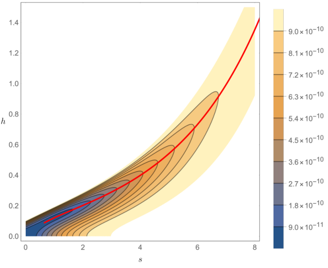
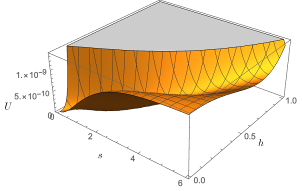
In this letter, we address the PBH production in Higgs-$R^{2}$ inflation. PBH production in the framework of single field critical Higgs inflation has been studied by many authors, but problematic issues regarding slow-roll violation, rapid $\xi$-running do not allow a significant PBH abundance in the desired mass range [69, 70, 71, 72, 73, 74, 75]. Here, we study the exact dynamics of inflation and numerically evaluate perturbation evading the problems regarding the validity of slow-roll approximation and show the significant production of PBH. Intriguingly, considering collective contributions from the scalaron and the proper RG-running effects for SM couplings taking the latest results from the LHC run-2, notably the running top quark mass [76], allows a second plateau along the trajectory of the inflaton in addition to the plateau at large field values as depicted in figure 1 and results in a significant amount of primordial black holes in the dark matter desired mass range $(10^{-16},10^{-15})M_{\odot}$ while satisfying Planck 2018 inflation parameters [42, 43].

The action for the Higgs-$R^{2}$ inflation in the Jordan frame is given as

where the gravity action including the nonminimal coupling with the Higgs, $h$, in the unitary gauge and $R^{2}$ term is

The reduced Planck scale is $M_{P}=1/\sqrt{8\pi G}\simeq 2.4\times 10^{18}~{\rm GeV}$. The scalaron mass $M\mathrel{\hbox to0.0pt{\lower 4.0pt\hbox{\hskip 1.0pt$\sim$}\hss}\raise 1.0pt\hbox{$<$}}M_{P}/\xi$ is introduced to match the dimensionality. We take the running self coupling of the Higgs $\lambda\left(\mu\right)$ at a scale $\mu$.

The scalaron, $s$, is defined as

The action in Einstein frame is obtained by Weyl transformation $g_{\mu\nu}=e^{\Omega(s)}g^{J}_{\mu\nu}$ where two scalar fields, $(\phi^{a})=(s,h)$ appear in the scalar potential $U(\phi^{a})$ and the kinetic terms involve a nontrivial field space metric $G_{ab}$:

Explicitly, the field space metric is given for $(s,h)$ as

The equations of motion will in turn inherit effects from the metric $G_{ab}$ in ‘curved field space’:

with the covariant derivatives $D_{a}\phi^{b}=\partial_{a}\phi^{b}+\Gamma^{b}_{ca}\phi^{c}$, $\Gamma^{b}_{ca}=\frac{1}{2}G^{be}\left(\partial_{c}G_{ae}+\partial_{a}G_{ec}-\partial_{e}G_{ca}\right)$, $D_{t}=\dot{\phi}^{a}\nabla_{a}$.

There are 3 parameters $\left.(M,\xi,\lambda)\right|_{\mu}$ governing the inflationary dynamics, which all run in scale $\mu$ by the Standard Model interactions as well the scalaron interactions following the 1-loop beta functions [77, 78, 58, 63]

where $\alpha={M_{P}^{2}}/{12M^{2}}$ and $\beta_{\rm SM}$ is the Standard Model contribution [79]. Numerically the running effect of $\beta_{\lambda}$ turns out to be the most significant factor in our analysis.

Determining an appropriate expression for $\mu$ also remains a nontrivial process. For theories consisting a single scalar (i.e. Higgs), taking $\mu$ to be a function solely depending on that particular scalar is natural. The introduction of additional scalar degrees of freedom generally alters this choice of scale. Recalling the gravity sector (2.2), obtaining an appropriate $\mu$ involves solving an equation that sets the logarithmic correction terms to be zero in order to guarantee perturbativity in the system [80, 81, 82, 78]. This also leads to a possible parameterization

For our parameters of interest, which satisfy Planck CMB observations and the desired PBH mass range, the Higgs field value during inflation $h\sim\mathcal{O}\left(0.1\right)-\mathcal{O}\left(1\right)M_{P}$, where the Hubble parameter $H\sim\sqrt{U}\sim 10^{-5}M_{P}$ and coefficients $a,b$ are numerical values with equal orders. Numerical solutions of this parameterization with desired values allow us to choose $\mu=h$ as our prescription. Therefore, we express $\lambda\left(\mu\right)$ as

with $\beta_{2}^{\text{SM}}\approx 0.5$,   $\mu_{\text{min}}=h_{\text{min}}\sim 10^{17}-10^{18}\,\,\text{GeV}$ as denoted in [83, 84]. ³³ 3 In this letter, we assume $\lambda_{\rm min}>0$ to guarantee the stability of the Higgs potential during inflation. This assumption is still consistent within $2\sigma$ with the currently available value for the pole mass, the correct parameter for RG analysis: $\left.m_{t}^{\rm pole}\right|_{\rm PDG}=173.1\pm 0.9~{\rm GeV}$ [85]. Current experimental and theoretical studies contain large uncertainties on identifying the parameter in Monte-Carlo simulation code as the pole mass [86].

We show the shape of the potential in figure 1. It also depicts the corresponding inflaton trajectory for given benchmark parameters. The potential exhibits a valley like structure, and the inflaton falls into this region and rolls along this trajectory, passing through the near inflection point as we already mentioned before. Along the trajectory, the time evolution can be effectively described in term of e-foldings, which is depicted in figure 2.

Due to the multifield potential of our setup, it is crucial to issue the production of isocurvature perturbations and its possible effects on large and small scale observables. The valley structure produces an isocurvature mass $m_{\text{iso}}^{2}=U_{NN}+\epsilon H^{2}{\rm I\!R}-\dot{\theta^{2}}$ with $U_{NN}=N^{a}N^{b}\nabla_{a}\nabla_{b}U$, $N_{a}$ the unit isocurvature direction vector, $\dot{\theta}=U_{N}/G_{ab}\dot{\phi^{a}}\dot{\phi^{b}}$ the turn rate, and I​R is the Ricci scalar for $G_{ab}$ [87, 66]. The appropriate parameters exhibit $m_{\text{iso,CMB}}^{2}\sim\mathcal{O}\left(10^{3}\right)H^{2}\gg H^{2}$ and negligible $\dot{\theta}$, leading to exponentially decaying isocurvature modes for $\mathcal{P}_{\text{iso}}\left(k_{\text{CMB}},N_{\text{end}}\right)/\mathcal{P}_{\mathcal{R}}\left(k_{\text{CMB}},N_{\text{end}}\right)\sim\mathcal{O}\left(10^{-7}\right)$ and effectively no superhorizon evolution from isocurvature sourcing ⁴⁴ 4 Here we follow the definitions for $\mathcal{P}_{\mathcal{R}},\mathcal{P}_{\text{iso}},\mathcal{P}_{\text{sourcing}}$ from the literature [88]. . For small scales, the inflaton’s kinetic energy substantially decreases when it reaches the near inflection point, remaining in this position for $\mathcal{O}\left(10\right)$ e-folds. This decreased kinetic energy in the USR phase implies $|\eta|\gg 1$, leading to superhorizon evolution of the curvature perturbation [89, 90, 91, 92, 93]. This is precisely where $\mathcal{P}_{\mathcal{R}}\left(k\right)$ enhances up to PBH criteria. Even in this region, $m_{\text{iso, PBH}}^{2}\sim\mathcal{O}\left(10^{4}\right)H^{2}$ and negligible $\dot{\theta}$ makes isocurvature sourcing negligible compared to the USR superhorizon growth with $\mathcal{P}_{\text{iso}}\left(k_{\text{USR}},N_{\text{end}}\right)/\mathcal{P}_{\mathcal{R}}\left(k_{\text{USR}},N_{\text{end}}\right)\approx\mathcal{P}_{\text{sourcing}}\left(k_{\text{USR}},N_{\text{end}}\right)/\mathcal{P}_{\mathcal{R}}\left(k_{\text{USR}},N_{\text{end}}\right)\sim\mathcal{O}\left(10^{-10}\right)$.

As our scenario requires, the potential needs to be close but still deviate from a true inflection point. The position of inflection and the corresponding value $\lambda_{\text{min}}^{\text{inf}}$ are determined for a given $M,~\xi,~\beta_{2},~h_{\text{min}}$ by computing

with the curved field space taken into account in the derivatives at the pivot point $(s,h)=(s^{*},h^{*})$. We then compute the $\lambda_{\text{min}}$ value, which encapsulates the information from the SM measurements, especially from $m_{t}$, $\alpha_{s}$ and also $m_{h}$, by subtracting an infinitesimal quantity from the inflection point value, $\lambda_{\text{min}}=\lambda_{\text{min}}^{\text{inf}}-\delta c$, with $\delta c\sim\mathcal{O}\left(10^{-7}\right)$ varying to induce a local minimum according to the criteria $\mathcal{P}_{\mathcal{R}}\left(k_{\text{PBH}}\right)\sim\mathcal{O}\left(10^{-2}\right)$.

We numerically evaluate the $\mathcal{P}_{\mathcal{R}}\left(k\right)$ using PyTransport [94] based on the $\delta N$ formalism implemented transport method [95, 96]. This inhibits the exact dynamics from (2.7) including effects of the ultra-slow-roll phase. Figure 3 delineates $\mathcal{P}_{\mathcal{R}}\left(k\right)$ from CMB horizon exit to inflation termination for the inflection point and local minimum cases with our benchmark cases (i) $\lambda_{\text{min}}^{\text{inf}}\approx 4.16\times 10^{-6}$, and (ii) $~\lambda_{\text{min}}\approx 4.10\times 10^{-6}$ for $M=4.2\times 10^{-5}M_{P},~h_{\text{min}}=0.15M_{P},~\xi=79$. Both cases exhibit a nearly scale invariant spectrum in small $k$ values, satisfying the observed Planck value $\mathcal{P}_{\mathcal{R}}\left(k_{\text{CMB}}\right)\approx 2.1\times 10^{-9}$. In this region, contributions from $\lambda\left(h\right)h^{4}/4$ become negligible, hence the potential for both cases take an approximate form $U\approx\frac{3}{4}M_{P}^{2}M^{2}e^{-2\Omega(s)}\left(e^{\Omega(s)}-1-{\xi h^{2}}/{M_{P}^{2}}\right)^{2}$, containing an exponentially suppressed term resulting in a plateau in CMB scales [43]. The peak enhancement behavior strongly depends on effects deviating from slow-roll [73, 89]. Compared to (i), where the slow-roll violating field evolution is not substantial enough, the shallow local minimum induced in (ii) allows the kinetic energy of the inflaton to significantly decrease, resulting in a severe growth in $\mathcal{P}_{\mathcal{R}}\left(k\right)$ up to $\mathcal{O}\left(10^{-2}\right)$.

The curvature perturbations exceeding the critical value collapse during horizon re-entry in the radiation dominated (RD) era [97, 14]. Hence the PBH mass is proportional to the corresponding horizon mass, $M_{H}=(2GH)^{-1}$ [98]

where $\gamma$ denotes the efficiency of collapse and has a typical value of $\gamma=0.2$ and the mass is in solar mass units.

We follow the ‘peaks theory’ method counting the number density of peaks above a given criterion [98, 99] to compute the PBH mass fraction $\beta_{M_{\text{PBH}}}$ of the universe and the PBH dark matter abundance $f_{\text{PBH}}\equiv\Omega_{\text{PBH}}/\Omega_{\text{DM}}$ (see also [100, 101, 98, 102, 103, 104]):

where $g_{*}=106.75$ is the effective relativistic degree of freedom in the RD era, $\Delta=\delta\rho/\rho$ and $\nu=\Delta/\sigma_{\Delta}$. $\Delta_{c}$ values for the RD era range alter with the feature of the inflationary power spectrum, however conventional values range in $\Delta_{c}\sim 0.3-0.5$ [98, 102, 105].

Figure 4 depicts $f_{\text{PBH}}$ for several cases, along with current observational constraints on this quantity.⁵⁵ 5 For extended mass functions, the constraints become more stringent in general [107], however for our scenario the bounds do not change significantly. Revisited bounds on $f_{\text{PBH}}$ allow the PBH mass range of $3.5\times 10^{-17}<M_{\rm PBH}/M_{\odot}<4\times 10^{-12}$ [108]. The peak itself exhibits an asymmetric form, which corresponds to the asymmetric growth and decay of $\mathcal{P}_{\mathcal{R}}\left(k\right)$ in small scales. Taking a reasonable $\Delta_{c}$ value, $f_{\text{PBH}}$ peaks with a value of approximately $f_{\text{PBH}}^{\text{peak}}\sim\mathcal{O}\left(0.1-1\right)$ in a mass range $M_{\text{PBH}}\sim\mathcal{O}\left(10^{-16}\right)-\mathcal{O}\left(10^{-12}\right)M_{\odot}$, covering all of the range allowed for PBHs to dominate as dark matter. This particular mass range directly corresponds to the target range for future femtolensing and GW observatories [13, 109, 110] allowing our scenario to be extensively tested to a significant level.

We depict the parameters $n_{s}$ and $M_{\text{PBH}}$ in figure 5 for parameter choices that satisfy the appropriate $\mathcal{P}_{\mathcal{R}}\left(k_{\text{CMB}}\right)$ value, an inflationary period of about 50-65 e-folds, and $\mathcal{P}_{\mathcal{R}}\left(k_{\text{peak}}\right)\sim\mathcal{O}\left(10^{-2}\right)$. Here the $n_{s}$ parameter is the spectral index of the comoving curvature power spectrum expressed as $n_{s}=1+d\ln\mathcal{P}_{\mathcal{R}}\left(k\right)/{d\ln k}$. From this we clearly notice a correlation between $n_{s}$ and $M_{\text{PBH}}$. This is expected as the $k_{\text{PBH}}$ is governed by the position of the shallow local minimum, in which parameters $h_{\text{min}}$, $\xi$ mainly determine. When fixing $h_{\text{min}}$, increasing $\xi$ shifts this local minimum to a larger field value, resulting in a heavier $M_{\text{PBH}}$. This in turn leads to a shorter period of slow-roll inflation before $\mathcal{P}_{\mathcal{R}}\left(k\right)$ increases, eventually giving a smaller $n_{s}$ value.

Our results indicate that albeit the scenario can produce enhanced $\mathcal{P}_{\mathcal{R}}\left(k\right)$ values for $M_{\text{PBH}}\sim\mathcal{O}\left(10^{-17}\right)-\mathcal{O}\left(10^{-11}\right)M_{\odot}$, consistency with Planck CMB observables restrain the possible mass range to the smaller limit, $\mathcal{O}\left(10^{-16}\right)-\mathcal{O}\left(10^{-15}\right)M_{\odot}$ within 2$\sigma$ significance with Planck. It also confines the possible $h_{\text{min}}$ range, which is in direct relation with the top quark pole mass in the renormalization group equations. This result is significantly enhanced from the single field critical Higgs inflation scenario [69, 111] in terms of both the achievable perturbation strength and the allowable parameter space. The addition of the $R^{2}$ term i.e. the scalaron degree thus allows the required $\mathcal{P}_{\mathcal{R}}\left(k\right)$ criteria with higher consistency with CMB measurements.

We report significant PBH production in Higgs-$R^{2}$ inflation with the Standard Model parameters obtained from the latest LHC run-2 results : running coupling of $\lambda\left(\mu\right)$ with an $R^{2}$ term allow two plateaus of the inflaton potential where the higher one is responsible for explaining CMB observations and the shallow local minimum in smaller field values is responsible for PBH production. The second region significantly amplifies the comoving curvature power spectrum resulting in an amplification of $\mathcal{P}_{\mathcal{R}}\left(k_{\text{PBH}}\right)/\mathcal{P}_{\mathcal{R}}\left(k_{\text{CMB}}\right)\sim\mathcal{O}\left(10^{7}\right)$ and stimulates gravitational collapse during horizon re-entry in the radiation dominated era, leading to PBHs with specific mass $M_{\rm PBH}\in(10^{-16},10^{-15})M_{\odot}$ consisting a significant fraction of dark matter. Our analysis point out that unlike single field critical Higgs inflation, which is unable to amplify $\mathcal{P}_{\mathcal{R}}\left(k\right)$ in the desired mass range, the addition of $R^{2}$ allows significant amplification in higher mass ranges that can remain as PBHs as the majority of dark matter up to our present universe.

We briefly comment on higher consistency with current CMB measurements and compatible PBH mass ranges, which are achievable when higher order terms, such as $R^{3},R^{4},\cdots$ are taken into account. These terms, which are natural in the sense of an EFT, will modify the $n_{s}$ predictions while keeping the $\mathcal{P}_{\mathcal{R}}(k_{\text{PBH}})$ profile effectively constant, shifting to central values of CMB data [31, 112].

This study opens up many interesting aspects. First, the detectability of this scenario also has advantages over others. Due to the tight correlation between $n_{s}$ and the mass of PBH, future CMB experiments will be able to determine this case in a relatively near future. The relation between the top quark mass and the PBH mass is also a strong correlation in the SM, therefore the observation of a PBH in the predicted mass may highly constrain the top quark pole mass. New physics incorporating both curved spacetime and additional degrees can change the high energy running behavior of $\lambda\left(\mu\right)$, which may affect the PBH mass and CMB observations. The cross confirmation between PBHs and CMB analysis may provide a good probe for BSM physics. The nontrivial contribution of gravity operators to Higgs inflation in terms of curvature perturbations is also a crucial point of our study, where other well-motivated terms also may lead to many interesting phenomena.

We thank Fedor Bezrukov, Kohei Kamada, Kazunori Kohri, Shi Pi, Misao Sasaki, and Jinsu Kim for helpful discussions on the possibility and computation of this setup. This work was supported by the National Research Foundation grants funded by the Korean government (MSIP) (NRF-2018R1A4A1025334)&(NRF-2019R1A2C1089334) (SCP) and (NRF-2020R1A6A3A13076216) (SML). SML was supported in part by the Hyundai Motor Chung Mong-Koo Foundation.

References

- [1] Y.B. Zel’dovich and I.D. Novikov, The Hypothesis of Cores Retarded during Expansion and the Hot Cosmological Model, Soviet Astronomy 10 (1966) 602.
- [2] S. Hawking, Gravitationally collapsed objects of very low mass, Mon. Not. Roy. Astron. Soc. 152 (1971) 75.
- [3] P. Ivanov, P. Naselsky and I. Novikov, Inflation and primordial black holes as dark matter, Phys. Rev. D50 (1994) 7173.
- [4] D. Blais, C. Kiefer and D. Polarski, Can primordial black holes be a significant part of dark matter?, Phys. Lett. B535 (2002) 11 [astro-ph/0203520].
- [5] N. Afshordi, P. McDonald and D.N. Spergel, Primordial black holes as dark matter: The Power spectrum and evaporation of early structures, Astrophys. J. 594 (2003) L71 [astro-ph/0302035].
- [6] M.Y. Khlopov, Primordial Black Holes, Res. Astron. Astrophys. 10 (2010) 495 [0801.0116].
- [7] P.H. Frampton, M. Kawasaki, F. Takahashi and T.T. Yanagida, Primordial Black Holes as All Dark Matter, JCAP 1004 (2010) 023 [1001.2308].
- [8] M. Sasaki, T. Suyama, T. Tanaka and S. Yokoyama, Primordial Black Hole Scenario for the Gravitational-Wave Event GW150914, Phys. Rev. Lett. 117 (2016) 061101 [1603.08338].
- [9] B. Carr, F. Kuhnel and M. Sandstad, Primordial Black Holes as Dark Matter, Phys. Rev. D94 (2016) 083504 [1607.06077].
- [10] K. Inomata, M. Kawasaki, K. Mukaida, Y. Tada and T.T. Yanagida, Inflationary Primordial Black Holes as All Dark Matter, Phys. Rev. D96 (2017) 043504 [1701.02544].
- [11] B. Carr and J. Silk, Primordial Black Holes as Generators of Cosmic Structures, Mon. Not. Roy. Astron. Soc. 478 (2018) 3756 [1801.00672].
- [12] H. Niikura et al., Microlensing constraints on primordial black holes with Subaru/HSC Andromeda observations, Nat. Astron. 3 (2019) 524 [1701.02151].
- [13] A. Katz, J. Kopp, S. Sibiryakov and W. Xue, Femtolensing by Dark Matter Revisited, JCAP 1812 (2018) 005 [1807.11495].
- [14] B.J. Carr, K. Kohri, Y. Sendouda and J. Yokoyama, New cosmological constraints on primordial black holes, Phys. Rev. D81 (2010) 104019 [0912.5297].
- [15] B.J. Carr, K. Kohri, Y. Sendouda and J. Yokoyama, Constraints on primordial black holes from the Galactic gamma-ray background, Phys. Rev. D94 (2016) 044029 [1604.05349].
- [16] R. Laha, Primordial black holes as dark matter candidate are severely constrained by the Galactic Center 511 keV gamma-ray line, 1906.09994.
- [17] M. Ricotti, J.P. Ostriker and K.J. Mack, Effect of Primordial Black Holes on the Cosmic Microwave Background and Cosmological Parameter Estimates, Astrophys. J. 680 (2008) 829 [0709.0524].
- [18] D. Aloni, K. Blum and R. Flauger, Cosmic microwave background constraints on primordial black hole dark matter, JCAP 1705 (2017) 017 [1612.06811].
- [19] V. Poulin, P.D. Serpico, F. Calore, S. Clesse and K. Kohri, CMB bounds on disk-accreting massive primordial black holes, Phys. Rev. D96 (2017) 083524 [1707.04206].
- [20] M. Kawasaki, N. Sugiyama and T. Yanagida, Primordial black hole formation in a double inflation model in supergravity, Phys. Rev. D57 (1998) 6050 [hep-ph/9710259].
- [21] K. Kohri, D.H. Lyth and A. Melchiorri, Black hole formation and slow-roll inflation, JCAP 0804 (2008) 038 [0711.5006].
- [22] M. Drees and E. Erfani, Running-Mass Inflation Model and Primordial Black Holes, JCAP 1104 (2011) 005 [1102.2340].
- [23] D.H. Lyth, Primordial black hole formation and hybrid inflation, 1107.1681.
- [24] M. Kawasaki, N. Kitajima and T.T. Yanagida, Primordial black hole formation from an axionlike curvaton model, Phys. Rev. D87 (2013) 063519 [1207.2550].
- [25] K. Kohri, C.-M. Lin and T. Matsuda, Primordial black holes from the inflating curvaton, Phys. Rev. D87 (2013) 103527 [1211.2371].
- [26] K. Belotsky, A. Dmitriev, E. Esipova, V. Gani, A. Grobov, M.Y. Khlopov et al., Signatures of primordial black hole dark matter, Mod. Phys. Lett. A 29 (2014) 1440005 [1410.0203].
- [27] S. Clesse and J. García-Bellido, Massive Primordial Black Holes from Hybrid Inflation as Dark Matter and the seeds of Galaxies, Phys. Rev. D92 (2015) 023524 [1501.07565].
- [28] J. Garcia-Bellido and E. Ruiz Morales, Primordial black holes from single field models of inflation, Phys. Dark Univ. 18 (2017) 47 [1702.03901].
- [29] G. Ballesteros and M. Taoso, Primordial black hole dark matter from single field inflation, Phys. Rev. D97 (2018) 023501 [1709.05565].
- [30] K. Inomata, M. Kawasaki, K. Mukaida and T.T. Yanagida, Double inflation as a single origin of primordial black holes for all dark matter and LIGO observations, Phys. Rev. D97 (2018) 043514 [1711.06129].
- [31] S. Pi, Y.-l. Zhang, Q.-G. Huang and M. Sasaki, Scalaron from -gravity as a heavy field, JCAP 1805 (2018) 042 [1712.09896].
- [32] K. Kohri and T. Terada, Primordial Black Hole Dark Matter and LIGO/Virgo Merger Rate from Inflation with Running Spectral Indices: Formation in the Matter- and/or Radiation-Dominated Universe, Class. Quant. Grav. 35 (2018) 235017 [1802.06785].
- [33] Y.-F. Cai, X. Tong, D.-G. Wang and S.-F. Yan, Primordial Black Holes from Sound Speed Resonance during Inflation, Phys. Rev. Lett. 121 (2018) 081306 [1805.03639].
- [34] K.M. Belotsky, V.I. Dokuchaev, Y.N. Eroshenko, E.A. Esipova, M.Y. Khlopov, L.A. Khromykh et al., Clusters of primordial black holes, Eur. Phys. J. C 79 (2019) 246 [1807.06590].
- [35] S. Passaglia, W. Hu and H. Motohashi, Primordial black holes and local non-Gaussianity in canonical inflation, Phys. Rev. D99 (2019) 043536 [1812.08243].
- [36] K. Dimopoulos, T. Markkanen, A. Racioppi and V. Vaskonen, Primordial Black Holes from Thermal Inflation, JCAP 1907 (2019) 046 [1903.09598].
- [37] S.S. Mishra and V. Sahni, Primordial Black Holes from a tiny bump in the Inflaton potential, 1911.00057.
- [38] R.-G. Cai, Z.-K. Guo, J. Liu, L. Liu and X.-Y. Yang, Primordial black holes and gravitational waves from parametric amplification of curvature perturbations, 1912.10437.
- [39] M. Sasaki, T. Suyama, T. Tanaka and S. Yokoyama, Primordial black holes—perspectives in gravitational wave astronomy, Class. Quant. Grav. 35 (2018) 063001 [1801.05235].
- [40] F.L. Bezrukov and M. Shaposhnikov, The Standard Model Higgs boson as the inflaton, Phys. Lett. B659 (2008) 703 [0710.3755].
- [41] A.A. Starobinsky, A New Type of Isotropic Cosmological Models Without Singularity, Phys. Lett. 91B (1980) 99.
- [42] Planck collaboration, Planck 2018 results. VI. Cosmological parameters, 1807.06209.
- [43] Planck collaboration, Planck 2018 results. X. Constraints on inflation, 1807.06211.
- [44] S.C. Park and S. Yamaguchi, Inflation by non-minimal coupling, JCAP 0808 (2008) 009 [0801.1722].
- [45] C.P. Burgess, H.M. Lee and M. Trott, Power-counting and the Validity of the Classical Approximation During Inflation, JHEP 09 (2009) 103 [0902.4465].
- [46] J.L.F. Barbon and J.R. Espinosa, On the Naturalness of Higgs Inflation, Phys. Rev. D79 (2009) 081302 [0903.0355].
- [47] C.P. Burgess, H.M. Lee and M. Trott, Comment on Higgs Inflation and Naturalness, JHEP 07 (2010) 007 [1002.2730].
- [48] R.N. Lerner and J. McDonald, Higgs Inflation and Naturalness, JCAP 1004 (2010) 015 [0912.5463].
- [49] S.C. Park and C.S. Shin, Clockwork inflation with non-minimal coupling, Eur. Phys. J. C79 (2019) 529 [1807.09952].
- [50] F. Bezrukov, A. Magnin, M. Shaposhnikov and S. Sibiryakov, Higgs inflation: consistency and generalisations, JHEP 01 (2011) 016 [1008.5157].
- [51] Y. Hamada, H. Kawai, K.-y. Oda and S.C. Park, Higgs Inflation is Still Alive after the Results from BICEP2, Phys. Rev. Lett. 112 (2014) 241301 [1403.5043].
- [52] F. Bezrukov and M. Shaposhnikov, Higgs inflation at the critical point, Phys. Lett. B734 (2014) 249 [1403.6078].
- [53] Y. Hamada, H. Kawai, K.-y. Oda and S.C. Park, Higgs inflation from Standard Model criticality, Phys. Rev. D91 (2015) 053008 [1408.4864].
- [54] G.F. Giudice and H.M. Lee, Unitarizing Higgs Inflation, Phys. Lett. B694 (2011) 294 [1010.1417].
- [55] J.L.F. Barbon, J.A. Casas, J. Elias-Miro and J.R. Espinosa, Higgs Inflation as a Mirage, JHEP 09 (2015) 027 [1501.02231].
- [56] G.F. Giudice and H.M. Lee, Starobinsky-like inflation from induced gravity, Phys. Lett. B733 (2014) 58 [1402.2129].
- [57] Y. Ema, Higgs Scalaron Mixed Inflation, Phys. Lett. B770 (2017) 403 [1701.07665].
- [58] D. Gorbunov and A. Tokareva, Scalaron the healer: removing the strong-coupling in the Higgs- and Higgs-dilaton inflations, Phys. Lett. B788 (2019) 37 [1807.02392].
- [59] A. Salvio and A. Mazumdar, Classical and Quantum Initial Conditions for Higgs Inflation, Phys. Lett. B750 (2015) 194 [1506.07520].
- [60] X. Calmet and I. Kuntz, Higgs Starobinsky Inflation, Eur. Phys. J. C76 (2016) 289 [1605.02236].
- [61] Y.-C. Wang and T. Wang, Primordial perturbations generated by Higgs field and operator, Phys. Rev. D96 (2017) 123506 [1701.06636].
- [62] D.M. Ghilencea, Two-loop corrections to Starobinsky-Higgs inflation, Phys. Rev. D98 (2018) 103524 [1807.06900].
- [63] Y. Ema, Dynamical Emergence of Scalaron in Higgs Inflation, JCAP 1909 (2019) 027 [1907.00993].
- [64] D.D. Canko, I.D. Gialamas and G.P. Kodaxis, A simple deformation of Starobinsky inflationary model, 1901.06296.
- [65] M. He, R. Jinno, K. Kamada, S.C. Park, A.A. Starobinsky and J. Yokoyama, On the violent preheating in the mixed Higgs- inflationary model, Phys. Lett. B791 (2019) 36 [1812.10099].
- [66] M. He, A.A. Starobinsky and J. Yokoyama, Inflation in the mixed Higgs- model, JCAP 1805 (2018) 064 [1804.00409].
- [67] A. Gundhi and C.F. Steinwachs, Scalaron-Higgs inflation, 1810.10546.
- [68] Y. Ema, R. Jinno, K. Mukaida and K. Nakayama, Violent Preheating in Inflation with Nonminimal Coupling, JCAP 1702 (2017) 045 [1609.05209].
- [69] J.M. Ezquiaga, J. Garcia-Bellido and E. Ruiz Morales, Primordial Black Hole production in Critical Higgs Inflation, Phys. Lett. B776 (2018) 345 [1705.04861].
- [70] K. Kannike, L. Marzola, M. Raidal and H. Veermäe, Single Field Double Inflation and Primordial Black Holes, JCAP 1709 (2017) 020 [1705.06225].
- [71] C. Germani and T. Prokopec, On primordial black holes from an inflection point, Phys. Dark Univ. 18 (2017) 6 [1706.04226].
- [72] F. Bezrukov, M. Pauly and J. Rubio, On the robustness of the primordial power spectrum in renormalized Higgs inflation, JCAP 1802 (2018) 040 [1706.05007].
- [73] H. Motohashi and W. Hu, Primordial Black Holes and Slow-Roll Violation, Phys. Rev. D96 (2017) 063503 [1706.06784].
- [74] I. Masina, Ruling out Critical Higgs Inflation?, Phys. Rev. D98 (2018) 043536 [1805.02160].
- [75] M. Drees and Y. Xu, Overshooting, Critical Higgs Inflation and Second Order Gravitational Wave Signatures, 1905.13581.
- [76] CMS collaboration, Running of the top quark mass from proton-proton collisions at 13 TeV, 1909.09193.
- [77] A. Codello and R.K. Jain, On the covariant formalism of the effective field theory of gravity and leading order corrections, Class. Quant. Grav. 33 (2016) 225006 [1507.06308].
- [78] T. Markkanen, S. Nurmi, A. Rajantie and S. Stopyra, The 1-loop effective potential for the Standard Model in curved spacetime, JHEP 06 (2018) 040 [1804.02020].
- [79] A. De Simone, M.P. Hertzberg and F. Wilczek, Running Inflation in the Standard Model, Phys. Lett. B678 (2009) 1 [0812.4946].
- [80] M. Herranen, T. Markkanen, S. Nurmi and A. Rajantie, Spacetime curvature and the Higgs stability during inflation, Phys. Rev. Lett. 113 (2014) 211102 [1407.3141].
- [81] M. Herranen, A. Hohenegger, A. Osland and A. Tranberg, Quantum corrections to inflation: the importance of RG-running and choosing the optimal RG-scale, Phys. Rev. D95 (2017) 023525 [1608.08906].
- [82] L. Chataignier, T. Prokopec, M.G. Schmidt and B. Swiezewska, Single-scale Renormalisation Group Improvement of Multi-scale Effective Potentials, JHEP 03 (2018) 014 [1801.05258].
- [83] G. Degrassi, S. Di Vita, J. Elias-Miro, J.R. Espinosa, G.F. Giudice, G. Isidori et al., Higgs mass and vacuum stability in the Standard Model at NNLO, JHEP 08 (2012) 098 [1205.6497].
- [84] D. Buttazzo, G. Degrassi, P.P. Giardino, G.F. Giudice, F. Sala, A. Salvio et al., Investigating the near-criticality of the Higgs boson, JHEP 12 (2013) 089 [1307.3536].
- [85] Particle Data Group collaboration, Review of Particle Physics, Phys. Rev. D 98 (2018) 030001.
- [86] G. Corcella, The top-quark mass: challenges in definition and determination, Front. in Phys. 7 (2019) 54 [1903.06574].
- [87] A. Achucarro, V. Atal, S. Cespedes, J.-O. Gong, G.A. Palma and S.P. Patil, Heavy fields, reduced speeds of sound and decoupling during inflation, Phys. Rev. D86 (2012) 121301 [1205.0710].
- [88] Z. Lalak, D. Langlois, S. Pokorski and K. Turzynski, Curvature and isocurvature perturbations in two-field inflation, JCAP 07 (2007) 014 [0704.0212].
- [89] S.M. Leach, M. Sasaki, D. Wands and A.R. Liddle, Enhancement of superhorizon scale inflationary curvature perturbations, Phys. Rev. D64 (2001) 023512 [astro-ph/0101406].
- [90] S.-L. Cheng, W. Lee and K.-W. Ng, Superhorizon curvature perturbation in ultraslow-roll inflation, Phys. Rev. D 99 (2019) 063524 [1811.10108].
- [91] C.T. Byrnes, P.S. Cole and S.P. Patil, Steepest growth of the power spectrum and primordial black holes, JCAP 06 (2019) 028 [1811.11158].
- [92] P. Carrilho, K.A. Malik and D.J. Mulryne, Dissecting the growth of the power spectrum for primordial black holes, Phys. Rev. D 100 (2019) 103529 [1907.05237].
- [93] J. Liu, Z.-K. Guo and R.-G. Cai, An analytical approximation of the scalar spectrum in the ultra-slow-roll inflationary models, Phys. Rev. D 101 (2020) 083535 [2003.02075].
- [94] D.J. Mulryne and J.W. Ronayne, PyTransport: A Python package for the calculation of inflationary correlation functions, 1609.00381.
- [95] D.J. Mulryne, D. Seery and D. Wesley, Moment transport equations for the primordial curvature perturbation, JCAP 1104 (2011) 030 [1008.3159].
- [96] M. Dias, J. Elliston, J. Frazer, D. Mulryne and D. Seery, The curvature perturbation at second order, JCAP 1502 (2015) 040 [1410.3491].
- [97] B.J. Carr, The Primordial black hole mass spectrum, Astrophys. J. 201 (1975) 1.
- [98] A.M. Green, A.R. Liddle, K.A. Malik and M. Sasaki, A New calculation of the mass fraction of primordial black holes, Phys. Rev. D70 (2004) 041502 [astro-ph/0403181].
- [99] S. Young, C.T. Byrnes and M. Sasaki, Calculating the mass fraction of primordial black holes, JCAP 1407 (2014) 045 [1405.7023].
- [100] B.J. Carr, J.H. Gilbert and J.E. Lidsey, Black hole relics and inflation: Limits on blue perturbation spectra, Phys. Rev. D50 (1994) 4853 [astro-ph/9405027].
- [101] A.M. Green and A.R. Liddle, Constraints on the density perturbation spectrum from primordial black holes, Phys. Rev. D56 (1997) 6166 [astro-ph/9704251].
- [102] T. Harada, C.-M. Yoo and K. Kohri, Threshold of primordial black hole formation, Phys. Rev. D88 (2013) 084051 [1309.4201].
- [103] C. Germani and I. Musco, Abundance of Primordial Black Holes Depends on the Shape of the Inflationary Power Spectrum, Phys. Rev. Lett. 122 (2019) 141302 [1805.04087].
- [104] C.-M. Yoo, J.-O. Gong and S. Yokoyama, Abundance of primordial black holes with local non-Gaussianity in peak theory, JCAP 1909 (2019) 033 [1906.06790].
- [105] I. Musco, The threshold for primordial black holes: dependence on the shape of the cosmological perturbations, Phys. Rev. D100 (2019) 123524 [1809.02127].
- [106] B. Carr, K. Kohri, Y. Sendouda and J. Yokoyama, Constraints on Primordial Black Holes, 2002.12778.
- [107] B. Carr, M. Raidal, T. Tenkanen, V. Vaskonen and H. Veermäe, Primordial black hole constraints for extended mass functions, Phys. Rev. D96 (2017) 023514 [1705.05567].
- [108] P. Montero-Camacho, X. Fang, G. Vasquez, M. Silva and C.M. Hirata, Revisiting constraints on asteroid-mass primordial black holes as dark matter candidates, JCAP 1908 (2019) 031 [1906.05950].
- [109] S. Jung and T. Kim, GRB Lensing Parallax: Closing Primordial Black Hole Dark Matter Mass Gap, 1908.00078.
- [110] B. Dasgupta, R. Laha and A. Ray, Neutrino and positron constraints on spinning primordial black hole dark matter, 1912.01014.
- [111] S. Rasanen and E. Tomberg, Planck scale black hole dark matter from Higgs inflation, JCAP 1901 (2019) 038 [1810.12608].
- [112] D.Y. Cheong, H.M. Lee and S.C. Park, Beyond the Starobinsky model for inflation, Phys. Lett. B 805 (2020) 135453 [2002.07981].