EXTENDED MODELS OF FINITE AUTOMATA
by
Özlem Salehi Köken
B.S., Mathematics, Boğaziçi University, 2011
M.S., Computer Engineering, Boğaziçi University, 2013
Submitted to the Institute for Graduate Studies in
Science and Engineering in partial fulfillment of
the requirements for the degree of
Doctor of Philosophy
Graduate Program in Computer Engineering
Boğaziçi University
2019
ABSTRACT
Many of the numerous automaton models proposed in the literature can be regarded as a finite automaton equipped with an additional storage mechanism. In this thesis, we focus on two such models, namely the finite automata over groups and the homing vector automata.
A finite automaton over a group is a nondeterministic finite automaton equipped with a register that holds an element of the group . The register is initialized to the identity element of the group and a computation is successful if the register is equal to the identity element at the end of the computation after being multiplied with a group element at every step. We investigate the language recognition power of finite automata over integer and rational matrix groups and reveal new relationships between the language classes corresponding to these models. We examine the effect of various parameters on the language recognition power. We establish a link between the decision problems of matrix semigroups and the corresponding automata. We present some new results about valence pushdown automata and context-free valence grammars.
We also propose the new homing vector automaton model, which is a finite automaton equipped with a vector that can be multiplied with a matrix at each step. The vector can be checked for equivalence to the initial vector and the acceptance criterion is ending up in an accept state with the value of the vector being equal to the initial vector. We examine the effect of various restrictions on the model by confining the matrices to a particular set and allowing the equivalence test only at the end of the computation. We define the different variants of the model and compare their language recognition power with that of the classical models.
EXTENDED MODELS OF FINITE AUTOMATA
APPROVED BY:
| Prof. A. C. Cem Say | . |
| (Thesis Supervisor) | |
| Assoc. Prof. Özlem Beyarslan | . |
| Prof. Sema Fatma Oktuğ | . |
| Assoc. Prof. Tolga Ovatman | . |
| Prof. Can Özturan | . |
DATE OF APPROVAL: 12.06.2019
To the memory of my grandfather Hasan Salehi,
my great-grandmother Gülizar Burhanetin, and
my grandmother Mader Burhanettin…
ACKNOWLEDGEMENTS
First of all I would like to express my gratitude to my supervisor Prof. A. C. Cem Say for his guidance and support throughout my journey at Boğaziçi University. He has always been a source of inspiration for me and it is a great pleasure to be his student. I would also like to thank Abuzer Yakaryılmaz for his significant contributions to my thesis. His enthusiasm has always motivated and encouraged me.
I would like to thank my thesis committee members Prof. Can Özturan and Assoc. Prof. Özlem Beyarslan for their valuable feedbacks over the years and devoting their time to this research. I would like to thank Prof. Sema Fatma Oktuğ and Assoc. Prof. Tolga Ovatman for kindly accepting to be in my thesis jury and for their helpful comments.
I am grateful to Dr. Flavio D’Alessandro for our joint works and for sharing his knowledge. It was a great experience to work with him. I would like to thank professors Ryan O’Donnell, Alexandre Borovik and Igor Potapov for their helpful answers to my questions.
My gratitudes go to all members of the Department of Computer Engineering for providing such a nice environment. I would like to especially thank Prof. Pınar Yolum Birbil and Prof. Cem Ersoy for their kindness and support. I want to thank all past and current members of BM26 with whom I had the chance of working with.
I would like to thank Pelin Gürel for her valuable friendship all through these years.
I would like to offer my deepest gratitude to my grandfather İbrahim Burhanettin, my aunt Perihan Burhanettin, and my parent-in-law Nebahat Köken for their endless love and faith in me. I want to thank my sister Meltem Salehi for always being cheerful and motivating me. I am indebted to my parents Feryal and Mecid Salehi for all their efforts and generosity which made this thesis possible. Finally I would like to express my love and gratitude to my husband Oktay Köken for his patience, guidance and encouragement and to my lovely daughter Eda for bringing joy to my life. Without them, it would have no meaning.
This work is supported by Boğaziçi University Research Fund Grant Number 11760 and by Scientific and Technical Research Council of Turkey (TÜBİTAK) BİDEB Scholarhip Program.
ÖZET
GÜÇLENDİRİLMİŞ SONLU DURUMLU MAKİNE MODELLERİ
Literatürde ortaya sürülmüş olan pek çok makine, bir sonlu durumlu makinenin ek bir hafıza ünitesi ile güçlendirilmiş hali olarak düşünülebilir. Bu tezde, bu makine-
lerden ikisine, gruplar üzerinde tanımlı sonlu durumlu makinelere ve eve dönen vektör makinelerine odaklanılmıştır.
grubu üzerinde tanımlı bir makine, ek hafıza ünitesinde grubundan bir elemanı tutma hakkına sahip, belirlenimci olmayan bir sonlu durumlu makinedir. Başlangıçta hafıza ünitesinin değeri grubunun birim elemanıdır. Bir hesaplamanın başarılı sayılabilmesi için hafıza ünitesinin değeri, her adımda grubun bir elemanıyla çarpıldıktan sonra bitimde grubun birim elemanına eşit olmalıdır. Bu çalışmada tam sayılı ve rasyonel sayılı matris grupları üzerinde tanımlanan sonlu durumlu makinelerin tanıdıkları dil sınıfları incelenmiştir. Çeşitli parametrelerin makinelerin tanıma gücünü nasıl etkilediği araştırılmıştır. Matris yarıgruplarının karar verme problemleri ile ilintili makinelerinki arasında bir bağ kurulmuştur. Grup üzerinde tanımlı makinelerle ilişkili olan bazı modellerle ilgili yeni sonuçlar elde edilmiştir.
Yeni tanımladığımız eve dönen vektör makinesi, bir sonlu durumlu makinenin bir vektörle güçlendirilmesi ve bu vektöre her adımda bir matrisle çarpılma hakkı verilmesiyle ortaya çıkmıştır. Vektörün başlangıç vektörüne eşit olup olmadığı kontrol edilebilir ve makinenin kabul şartı, hesaplama bittiğinde vektörün başlangıç vektörüne eşit olması ve kabul durumlarından birinde bulunulmasıdır. Kullanılan matris kümesi sınırlanarak ve vektörün eşitlik kontrolünün sadece sonda gerçekleşmesine izin verilerek, farklı kısıtlamaların makineye olan etkisi incelenmiştir. Makinenin çeşitli sürümlerinin dil tanıma gücüyle klasik modellerin dil tanıma gücü karşılaştırılmıştır.
TABLE OF CONTENTS
LIST OF FIGURES
LIST OF TABLES
LIST OF SYMBOLS
| The identity element of a group/monoid | ||
| The cardinality of a set | ||
| A pushdown automaton | ||
| The entry in the ’th row and the ’th column of the matrix | ||
| The maximum such that there exist distinct strings that are pairwise -dissimilar for | ||
| B | The bicyclic monoid | |
| The set of all elements in which can be represented by a word of length at most | ||
| The Baumslag Solitar group | ||
| A counter automaton | ||
| The set of head directions | ||
| The identity element of a group/monoid | ||
| The base-10 number encoded by in base- | ||
| An extended finite automaton | ||
| A finite automaton | ||
| The free group of rank | ||
| A group | ||
| A context-free grammar | ||
| A context-free valence grammar | ||
| The growth function of a group | ||
| The general linear group of order over the field of rationals | ||
| The general linear group of order over the field of integers | ||
| The discrete Heisenberg group | ||
| Identity matrix | ||
| An ideal | ||
| A language | ||
| The complement of the language | ||
| The language generated by some grammar/recognized by some machine | ||
| The class of languages recognized by -automata | ||
| The class of languages recognized by strongly -time bounded -automata | ||
| The class of languages recognized by weakly -time bounded -automata | ||
| The class of languages recognized by the machine type | ||
| The class of languages generated by context-free valence grammars over | ||
| The class of languages recognized by valence automata over | ||
| The class of languages recognized by valence pushdown automata over | ||
| The class of languages generated by regular valence grammars over | ||
| M | The set of matrices multiplied with the vector of a homing vector automaton | |
| A monoid | ||
| The set of matrices with integer entries | ||
| The set of natural numbers | ||
| Little-o notation | ||
| Big-O notation | ||
| A valence pushdown automaton | ||
| The power set of a set | ||
| P2 | The polycyclic monoid of rank 2 | |
| The polycyclic monoid on | ||
| The set of rational numbers | ||
| The set/group of nonzero rational numbers | ||
| The set of states | ||
| . | The initial state | |
| The set of accept states | ||
| A semigroup | ||
| The Rees quotient semigroup | ||
| The set of matrices whose entries belong to the set for some positive integer | ||
| The special linear group of order over the field of rationals | ||
| The special linear group of order over the field of integers | ||
| A Turing machine | ||
| The maximum such that there exist distinct strings that are uniformly -dissimilar for | ||
| A vector | ||
| A vector automaton | ||
| The ’th entry of the vector | ||
| A finite automaton with multiplication | ||
| The length of the string | ||
| The word problem language of the group | ||
| The number of occurrences of in | ||
| The ’th symbol of the string | ||
| The reverse of the string | ||
| The set of integers | ||
| The set/group of -dimensional integer vectors | ||
| A transition function | ||
| The empty string | ||
| A tape/stack alphabet | ||
| The set of multipliers of a finite automaton with multiplication | ||
| A register status | ||
| The set of register status | ||
| The Parikh image of a language | ||
| The Parikh image of a string | ||
| A symbol | ||
| An alphabet | ||
| The set of all strings over | ||
| A counter status | ||
| The set of counter status | ||
| Isomorphic | ||
| Stay | ||
| Right | ||
| Left | ||
| Blank symbol | ||
| End-marker |
LIST OF ACRONYMS/ABBREVIATIONS
| 0-1DFAMW | Stateless one-way deterministic finite automaton with multiplication without equality |
| 0-DBHVA() | Stateless real-time -dimensional deterministic blind homing vector automaton |
| 0-DFAMW | Stateless real-time deterministic finite automaton with multiplication without equality |
| 0-DHVA() | Stateless real-time -dimensional deterministic homing vector automaton |
| 0-NBHVA() | Stateless real-time -dimensional nondeterministic blind homing vector automaton |
| 0-NFAMW | Stateless real-time nondeterministic finite automaton with multiplication without equality |
| 0-NHVA() | Stateless real-time -dimensional nondeterministic homing vector automaton |
| 1DBHVA() | One-way -dimensional deterministic blind homing vector automaton |
| 1DFA | One-way deterministic finite automaton |
| 1DFAM | One-way deterministic finite automaton with multiplication |
| 1DFAMW | One-way deterministic finite automaton with multiplication without equality |
| 1DHVA() | One-way -dimensional deterministic homing vector automaton |
| 1DBCA | One-way deterministic blind -counter automaton |
| 1DCA | One-way deterministic -counter automaton |
| 1NBHVA() | One-way -dimensional nondeterministic blind homing vector automaton |
| 1NHVA() | One-way -dimensional nondeterministic homing vector automaton |
| 1NFA | One-way nondeterministic finite automaton |
| 1NFAM | One-way nondeterministic finite automaton with multiplication |
| 1NFAMW | One-way nondeterministic finite automaton with multiplication without equality |
| 1NBCA | One-way nondeterministic blind -counter automaton |
| 1NCA | One-way nondeterministic -counter automaton |
| 1NPDA | One-way nondeterministic pushdown automaton |
| DBHVA() | Real-time -dimensional deterministic blind homing vector automaton |
| DFA | Real-time deterministic finite automaton |
| DFAM | Real-time deterministic finite automaton with multiplication |
| DFAMW | Real-time deterministic finite automaton with multiplication without equality |
| DHVA() | Real-time -dimensional deterministic homing vector automaton |
| DBCA | Real-time deterministic blind -counter automaton |
| DCA | Real-time deterministic -counter automaton |
| DVA() | Real-time -dimensional deterministic vector automaton |
| CA | Counter automaton |
| The class of context-free languages | |
| FA | Finite automaton |
| FAM | Finite automaton with multiplication |
| HVA() | -dimensional homing vector automaton |
| BCA | blind -counter automaton |
| CA | -counter automaton |
| NBHVA() | Real-time -dimensional nondeterministic blind homing vector automaton |
| NHVA() | Real-time -dimensional nondeterministic homing vector automaton |
| NBCA | Real-time nondeterministic blind -counter automaton |
| NCA | Real-time nondeterministic -counter automaton |
| NFA | Real-time nondeterministic finite automaton |
| NFAM | Real-time nondeterministic finite automaton with multiplication |
| NFAMW | Real-time nondeterministic finite automaton with multiplication without equality |
| PDA | Pushdown automaton |
| The class of recursively enumerable languages | |
| The class of regular languages | |
| The class of languages that can be decided by a deterministic Turing machine within time and space where is the length of the input | |
| TM | Turing machine |
Chapter 1 INTRODUCTION
1.1 Automata Theory
The theory of computation aims to investigate the computation process and tries to answer the question “What are the fundamental capabilities and limitations of computers?” as stated by Sipser [1]. To study the computation process, we have to first formalize the notions of computational problems and computational models.
At the heart of computational problems, lie the decision problems, the problems whose answers are either yes or no. Any decision problem can be represented by the set of instances which have the answer yes. Consider the problem of checking whether a number is prime. This problem can be represented by the set , where the members of the set are the prime numbers. Furthermore, the elements of the set can be represented as strings, a finite sequence of symbols belonging to a finite set called the alphabet. For instance, the set of prime numbers can be expressed by the set , where the alphabet contains the single symbol .
Automata theory is the study of computational models that solve decision problems. An automaton is as an abstract machine which processes an input string and makes the decision of yes or no, more technically called as acceptance or rejection. Automata allow us to formalize the notion of computation and serve as mathematical models for computing devices. The set of all accepted input strings is called the language recognized by the machine. If there exists a machine whose language is the set of yes instances of a problem, than we have a machine solving the problem.
The most basic model which is known as the finite automaton or finite state machine is an abstract model for computation with finite memory. It is assumed that the input string is written on a tape and the machine has a tape-head reading the string from left to right. There exist finitely many states and a set of rules governing the transitions between these states. Computation starts from a designated initial state and one input symbol is consumed at each step. An input string is accepted if after reading the string, computation ends in a special state called the accept state and otherwise rejected.
One of the founders of the theory of formal languages, Noam Chomsky, defined four classes of languages, namely the classes of regular languages, context-free languages, context-sensitive languages and recursively enumerable languages, forming the Chomsky Hierarchy. Finite automata recognize exactly the class of regular languages.
1.2 Extended Models of Finite Automata
Throughout the literature, a variety of automaton models has been proposed. Many different models of automata that have been examined can be regarded as a finite automaton augmented with some additional memory. The type of the memory, restrictions on how this memory is accessed, computation mode and the conditions for acceptance determine the expressiveness of the model in terms of language recognition. One can list pushdown automata [2], counter machines [3] and Turing machines [4] among the many such proposed models.
Pushdown automata are finite automata augmented with a stack, a memory which can be used in the last-in-first-out manner. Their nondeterministic variants, in which there may be more than one possible move at each step, and the acceptance condition is the existence of at least one computational path that ends in an accept state, recognize exactly the class of context-free languages. Note that a language is context-free if it is generated by a context-free grammar, which is a collection consisting of a set of variables and terminals, and a set of production rules. Starting from the start variable, the rules describe how to generate a string of terminals, by replacing each variable with a string of variables and terminals. The set of all generated strings is the language of the grammar.
The foundations of the theory of computation have been established by Alan Turing, who proposed the Turing machine as a model for universal computation [4]. A Turing machine is a finite automaton equipped with an infinite read-write tape which is allowed to move in both directions. The Turing machine is a model for our computers and for the computation process performed by the human mind. A language is recognized by a Turing machine if for every string in the language, the computation on the string ends in the accept state. The class of languages recognized by Turing machines is known as the recursively enumerable or Turing recognizable languages.
Counter machines are finite automata equipped with additional registers that are initialized to zero at the beginning and can be incremented or decremented based on the current state and the status of the counters (zero or nonzero) throughout the computation. A finite automaton with 2 counters is as powerful as a Turing machine, which led researchers to add various restrictions to the definition. For instance, in a blind counter automaton, the counters cannot be checked until the end of the computation and the next move depends only on the current state and the scanned symbol. The class of languages recognized by nondeterministic blind counter automata are incomparable with the class of context-free languages.
Another variant is the extended finite automaton (finite automaton over a group, group automaton, -automaton), which is a nondeterministic finite automaton equipped with a register that holds an element from a group [5]. The register is initialized to the identity element of the group, and a computation is deemed successful if the register is equal to the identity element at the end of the computation after being multiplied with a group element at every step. The computational power of a -automaton is determined by the group . This setup generalizes various models such as pushdown automata, Turing machines, nondeterministic blind counter automata and finite automata with multiplication [6]. When a monoid is used instead of a group, then the model is also called monoid automaton or -automaton. The same model also appears under the name of valence automata in various papers.
The notion of extended finite automata is also strictly related to that of valence grammar introduced by Pǎun in [7]. A valence grammar is a formal grammar in which every rule of the grammar is equipped with an element of a monoid called the valence of the rule. Words generated by the grammar are defined by successful derivations. A successful derivation is a derivation that starts from the start symbol of the grammar such that the product of the valences of its productions (taken in the obvious order) is the identity of the monoid. Valence pushdown automata, which are pushdown automata equipped with a register that is multiplied by elements from a monoid at each step, and context-free valence grammars are discussed in [8].
We have also introduced a new model called vector automaton in [9]. A vector automaton is a finite automaton which is endowed with a vector, and which can multiply this vector with an appropriate matrix at each step. One of the entries of this vector can be tested for equality to a rational number. The machine accepts an input string if the computation ends in an accept state, and the test for equivalence succeeds.
In order to incorporate the notion of the computation being successful if the register returns to its initial value at the end of the computation as in the case of extended finite automata to this setup, we propose the new homing vector automaton (HVA) model. A homing vector automaton can multiply its vector with an appropriate matrix at each step and can check the entire vector for equivalence to the initial value of the vector. The acceptance criterion is ending up in an accept state with the value of the vector being equal to the initial vector.
1.3 Contributions and Overview
The aim of this thesis is to investigate extended models of finite automata focusing mainly on finite automata over groups and homing vector automata. We examine the classes of languages that can be recognized by different variants of these models and compare them with the classes of languages recognized by the classical models. We prove separation results based on the different restrictions imposed on the models.
Much of the current literature on extended finite automata pays particular attention to finite automata over free groups and free Abelian groups. This study makes a major contribution to the research on extended finite automata by exploring finite automata over matrix groups for the first time. Most of these results were published in [10, 11, 12].
Matrices play an important role in many areas of computation and many important models of probabilistic and quantum computation [13, 14] can be viewed in terms of vectors being multiplied by matrices. The motivation behind analyzing homing vector automata is the matrix multiplication view of programming, which abstracts the remaining features of such models away. We investigate homing vector automata under several different regimes, which helps us to determine whether different parameters confer any additional recognition power. Our results on homing vector automata have previously appeared in [15, 16, 17].
We also present some results on context-free valence grammars and valence pushdown automata. These results are mainly some generalizations of the previously established results for the theory of extended finite automata and appeared in [18].
The rest of the thesis is structured as follows:
Chapter 2 contains definitions of basic terminology and formal definitions of some of the classical models. It provides a framework for the rest of the thesis. A background on algebra is also presented.
In Chapter 3, we investigate the language classes recognized by finite automata over matrix groups. For the case of matrices, we prove that the corresponding finite automata over rational matrix groups are more powerful than the corresponding finite automata over integer matrix groups. Finite automata over some special matrix groups, such as the discrete Heisenberg group and the Baumslag-Solitar group are also examined. We also introduce the notion of time complexity for group automata and demonstrate some separations among related classes. The case of linear-time bounds is examined in detail throughout our repertory of matrix group automata. Furthermore, we look at the connection between decision problems for matrix groups and finite automata over matrix groups.
Chapter 4 defines the homing vector automaton and introduces the various limited versions that we will use to examine the nature of the contribution of different aspects of the definition to the power of the machine. A generalized version of the Stern-Brocot encoding method, suitable for representing strings on arbitrary alphabets, is developed. The computational power and properties of deterministic, nondeterministic, blind, non-blind, real-time and one-way versions of these machines are examined and compared to various related types of automata. We establish a connection between one-way nondeterministic version of homing vector automata and extended finite automata. As one-way versions are too powerful even in the case of low dimensions, we pay special attention to real-time homing vector automata. Some closure properties of real-time homing vector automata and their stateless (one state) versions are investigated.
In Chapter 5, we focus on pushdown valence automata and context-free valence grammars. We investigate valence pushdown automata, and prove that they are only as powerful as valence automata. We observe that certain results proven for monoid automata can be easily lifted to the case of context-free valence grammars.
Chapter 6 is the conclusion of the thesis. We summarize the results and list some open questions which form a basis for future research.
Chapter 2 BACKGROUND
2.1 Basic Notation and Terminology
2.1.1 Sets
Let be a set. denotes the cardinality of . The power set of is denoted by . A subset is a linear set if there exist vectors such that
A semilinear set is a finite union of linear sets.
The Cartesian product of sets is the set of all ordered -tuples where for . The Cartesian product is denoted by either or by .
2.1.2 Strings and Languages
An alphabet is a finite set of symbols and usually it is denoted by . A string (word) over is obtained by concatenating zero or more symbols from . The string of length zero is called the empty string and denoted by . The set is denoted by in short. We denote by the set of all words over .
For a string , denotes its reverse, denotes its length, denotes its ’th symbol, denotes the number of occurrences of in .
A language is a set of strings over . For a given language , its complement is denoted by . For a given string , denotes the singleton language containing only .
For a string where is an ordered alphabet, the Parikh image of is defined as
For a language , its Parikh image is defined as
A language is called semilinear if is semilinear.
A language is said to be bounded if there exist words such that . A bounded language is said to be (bounded) semilinear if there exists a semilinear set of such that
2.1.3 Vectors and Matrices
For a given row vector , denotes its ’th entry. Let be a dimensional matrix. denotes the entry in the ’th row and ’th column of .
The identity matrix of size is the matrix with ones on the main diagonal and zeros elsewhere.
2.2 Automata and Computation
In this section, we are going to talk about basic notions of computation. We refer to the finite automaton model which may be extended with a storage mechanism as discussed in Section 1.1 and Section 1.2.
For a machine , there exist a finite set of states where is the initial state unless otherwise specified and a set of accept state(s) . An input string is written on a one-way infinite tape starting from the leftmost tape square. The transition function denoted by describes the next move of upon reading some input symbol. Initially, the tape-head is placed on the leftmost tape square. Starting from the initial state, the sequence of transitions performed by on any input string is called a computation.
The acceptance criteria of an input string depend on the type of the machine which we will discuss in detail in Section 2.3. A computation is called accepting if the computation results in the acceptance of the string, and rejecting otherwise. The set of all strings accepted by is called the language recognized by and denoted by .
2.2.1 Deterministic Computation
A computation is deterministic if there is only one possible move at each step. When an input string is read, there is only a single computation.
2.2.2 Nondeterministic Computation
In a nondeterministic computation, there may be more than one possible move at each step. When an input string is read, the computation looks like a tree since there may be more than one computation path.

2.2.3 Blind Computation
For the machine types which have additional storage mechanisms like registers or counters, computation is called blind if the status of the storage mechanism cannot be checked until the end of the computation. The next move of the machine is not affected by the current status of the storage mechanism. When the computation ends, the status of the storage mechanism is checked and it determines whether the input string will be accepted or not.
2.2.4 Empty String Transitions
When a machine makes an empty string () transition, it moves without consuming any input symbol. In deterministic machines, moves should be defined carefully as they may lead to nondeterminism.
2.2.5 Real-time, One-way and Two-way Computation
A computation is called real-time if the tape-head moves right at each step. A computation is called one-way if the tape-head is allowed to stay on the input tape while moving from left to right. This can be accomplished by adding an additional direction component to the transition function which dictates the movement of the tape-head. A computation is called two-way if the tape-head can move both left and right. Tape head directions will be specified by a subset of the set where , and stand for left, stay and right respectively.
Note that a machine making -transitions does not operate in real-time. A one-way nondeterministic computation may be also defined without specifying the head directions but allowing -moves instead. In that case, it is assumed that the machine moves right as long as it consumes an input symbol.
2.2.6 End-marker
In some models, the input string is written on the tape in the form and the machine is allowed to make transition(s) after finishing reading the input string, upon scanning the end-marker , which we call postprocessing. Postprocessing may add additional power depending on the model.
2.3 Classical Models
2.3.1 Finite Automaton
A finite automaton (FA) is a 5-tuple
where is the set of states, is the input alphabet, is the transition function, is the initial state and is the set of accept states. The transitions of depend only on the current state and the input symbol.
Formally, the transition function of a one-way deterministic finite automaton (1DFA) is defined as follows:
where is the set representing the possible moves of the tape-head, denoting stay and denoting right.
means that moves to state moving its tape-head in direction upon reading in state . We assume that the last move of the machine always moves the tape-head right.
In a real-time deterministic finite automaton (DFA), the tape-head moves right at every step and the direction component for the tape-head is omitted from the transition function:
Let us define the nondeterministic variants of finite automata. The transition function of a one-way nondeterministic finite automaton (1NFA) is defined as
so that there may be more than one possible move at each step and the machine is allowed to make -transitions.
A real-time nondeterministic finite automaton (NFA) is not allowed to perform any -transitions. The transition function of an NFA is defined as follows:
An input string of length is accepted by a finite automaton if there is a computation in which the machine enters an accept state with the tape-head on the ’st tape square.
1NFAs, 1DFAs, NFAs and DFAs recognize the same class of languages known as the class of regular languages, abbreviated by .
2.3.2 Pushdown Automaton
A pushdown automaton (PDA) is a finite automaton equipped with a stack. Stacks are one-way infinite storage mechanisms working in last-in-first-out fashion. The operations applied on a stack are called the pop and push operations, which stand for removing the topmost symbol from the stack and adding a new symbol on top of the stack by pushing down the other symbols in the stack, respectively. Note that the stack alphabet may be different than the input alphabet. At each step of the computation, the machine may pop the topmost symbol from the stack, move to a new state, and push a new symbol onto the stack, depending on the current state and the input symbol.
Formally, a one-way nondeterministic pushdown automaton (1NPDA) is a 6-tuple
where is the stack alphabet. The transition function of a 1NPDA is defined as
where . means when in state reading , pops from the stack, moves to state and pushes onto the stack. Note that and can be in which case nothing is popped from or pushed onto the stack. If is not on top of the stack, then the transition cannot take place.
A string of length is accepted by a 1NPDA if there exists a computation in which the machine enters an accept state with the tape-head on the ’st tape square and the stack is empty. There are also alternative definitions for acceptance which do not require an empty stack. By using -transitions, it is easy to see that the stack may be emptied in an accept state to satisfy the additional empty stack requirement and the two definitions correspond to the same class of languages, as long as the computation is one-way and -moves are possible.
1NPDAs recognize the class of context-free () languages.
2.3.3 Turing Machine
A Turing machine is a finite state automaton with the following properties:
- •
The tape-head can move in both directions.
- •
The tape-head can read from the tape and modify the tape content by writing on the tape.
At the beginning of the computation, the input is written on the tape starting from the first tape square and the rest of the tape contains the special blank symbol. If the tape-head tries to move left on the leftmost square, its position does not change.
Formally, a (two-way deterministic) Turing machine (TM) is a 7-tuple
where is the input alphabet not containing the blank symbol , is the tape alphabet where and , and are the accept and reject states respectively. The transition function of a TM is defined as follows:
where , meaning that moves to state , updating the tape square under the tape-head by , moving the tape-head in the direction , when in state and reading from the tape, specified by the transition .
While processing an input string, the computation may end at any point (before finishing reading the input string) in the designated accept state resulting in the acceptance of the input string, in the designated reject state resulting in the rejection of the input string or the computation may go on forever without ever entering the accept state or the reject state.
Turing machines recognize the class of recursively enumerable languages ().
2.3.4 Counter Automaton
A counter automaton (CA) is a finite automaton equipped with one or more counters, a storage mechanism holding an integer which can be incremented, decremented, and checked for equivalence to zero. Formally a CA is a 6-tuple
and a CA with counters is abbreviated as CA. At the beginning of the computation, counters are initialized to 0. At each step of the computation, depending on the current state and the status of the counters, moves to another state and updates its counters. .
The transition function of a one-way deterministic -counter automaton (1DCA) is defined as follows:
where and . A transition of the form means that upon reading in state , moves to updating its counters by and updates the tape-head with respect to , given that the status of the counters is , where and denote whether the corresponding counter values equal zero or not, respectively.
By restricting 1DCAs so that the status of the counters cannot be checked until the end of the computation, we obtain one-way deterministic blind -counter automaton (1DBCA). The transition function of a 1DBCA is formally defined as follows:
In a blind counter automaton, the next move of the machine does not depend on the status of the counters.
For the one-way deterministic machines, we assume that the last move of the machine always moves the tape-head to the right.
The real-time versions, real-time deterministic -counter automaton (DCA) and real-time deterministic blind -counter automaton (DBCA) are defined analogously, by omitting the direction component from the transition functions. The ranges of the transition functions take the following form: .
Let us define the nondeterministic variants of counter automata. The transition function of a one-way nondeterministic -counter automaton (1NCA) is defined as follows:
A one-way nondeterministic blind -counter automaton (1NBCA) is a restricted 1NCA which cannot check the value of the counters until the end of the computation. Transition function of a 1NBCA is defined as
The real-time versions, real-time nondeterministic -counter automaton (NCA) and real-time nondeterministic blind -counter automaton (NBCA) are defined analogously by not allowing -moves. The domains of the transition functions of these models are replaced with and respectively.
An input string of length is accepted by a CA if there exists a computation in which the machine enters an accept state with the tape-head on the ’st square. An input string is accepted by a BCA with the further requirement that all of the counters- values are equal to 0 .
The abbreviations used for counter automata variants discussed so far are given in Table 2.1.
| Real-time | One-way | |
|---|---|---|
| Deterministic | DCA | 1DCA |
| Deterministic blind | DBCA | 1DBCA |
| Nondeterministic | NCA | 1NCA |
| Nondeterministic blind | NBCA | 1NBCA |
A 1D2CA can simulate a Turing Machine [19] and therefore . As two counters are enough to recognize any recursively enumerable language, a considerable amount of literature has been published on language recognition power of counter automata under various restrictions. Preliminary work on counter automata was undertaken by Fischer et al., who investigated real-time deterministic counter automata [3], and one-way deterministic counter automata [20]. A hierarchy based on the number of the counters for real-time deterministic counter automata is demonstrated in [3]. In [20], the state set is separated into polling states from which the machine moves to another state and updates the counters by consuming an input symbol and autonomous states which allow machine to update the counters and change the state without reading anything. It is easy to show that both definitions are equivalent and correspond to machines with the same language recognition power.
A remarkable result from [20] states the following:
Fact 2.1.
[20] Given any CA with the ability to alter the contents of each counter independently by any integer between and in a single step (for some fixed integer ), one can effectively find a time-equivalent (ordinary) CA.
The proof involves using some additional states to simulate counter updates from the set with an ordinary counter automaton, without increasing the time complexity and the number of the counters. Hence, we can assume that any CA can be updated by arbitrary integers at each step.
One-way deterministic and nondeterministic counter automata working under time restrictions formed the central focus of study of Greibach in [21], in which the author proved various separation results between deterministic and nondeterministic models. Let us note that in [21] and [22] where one-way deterministic counter automata are investigated, it is assumed that the counter automata can process the end-marker.
In another major study by Greibach, one-way nondeterministic blind counter automata are examined [23] and some other restricted versions like partially blind counters and reversal bounded counters are introduced as well.
2.3.5 Finite Automata with Multiplication
A finite automaton with multiplication (FAM) [6] is 6-tuple
where the additional component is a finite set of rational numbers (multipliers). A FAM is a finite automaton equipped with a register holding a positive rational number. The register is initialized to 1 at the beginning of the computation and multiplied with a positive rational number at each step, based on the current state, input symbol and the status of the register determined by whether the register is equal to 1 or not. The input string of a FAM is given in the form and FAMs are allowed to perform post-processing.
The original definition of FAMs is given for one-way machines where the tape-head is allowed to stay on the same input symbol for more than one step.
A one-way deterministic finite automaton with multiplication (1DFAM) is defined by the transition function
where , is the set denoting the whether the register is equal to 1 or not respectively and is the set of head directions. It is assumed that for all so that the computation ends once the end-marker is scanned in an accept state. Reading symbol in state , compares the current value of the register with 1, thereby calculating the corresponding value , and switches its state to , moves its head in direction , and multiplies the register by , in accordance with the transition function value .
A one-way deterministic finite automaton with multiplication without equality (1DFAMW) is a model obtained by restricting 1DFAM so that the register can be checked only at the end of the computation. The transition function of a 1DFAMW is defined as follows:
where the next move of the machine does not depend on the current status of the register. The 1DFAMW can be seen as the blind version of the 1DFAM model.
We define the real-time versions, real-time deterministic finite automaton with multiplication (DFAM), and real-time deterministic finite automaton with multiplication without equality (DFAMW), by removing the direction component from the transition functions and assuming that the tape-head moves right at each step. The ranges of the transition functions are updated with .
A one-way nondeterministic finite automaton with multiplication (1NFAM) is a model that extends the 1DFAM with the ability to make nondeterministic moves. The transition function of a 1NFAM is defined as
A one-way nondeterministic finite automaton with multiplication without equality (1NFAMW) is the blind version of the 1NFAM model which cannot check whether or not the register has value 1 during computation. Transition function of a 1NFAMW is defined as follows:
so that the next move of the machine does not depend on the current status of the register.
We also define real-time versions real-time nondeterministic finite automaton with multiplication (NFAM) and real-time nondeterministic finite automaton with multiplication without equality (NFAMW) by removing the direction component from the transition functions and assuming that the tape-head moves right at each step. In that case, the ranges of the transition functions are updated with .
For an input string of length , is accepted by a FAM or a FAMW if there exists a computation in which the machine enters an accept state with the input head on the end-marker and the register is equal to 1.
The abbreviations used for finite automata with multiplication variants discussed so far are given in Table 2.2.
| Real-time | One-way | |
|---|---|---|
| Deterministic | DFAM | 1DFAM |
| Deterministic blind | DFAMW | 1DFAMW |
| Nondeterministic | NFAM | 1NFAMW |
| Nondeterministic blind | NFAMW | 1NFAMW |
The following characterization of the class of languages recognized by 1NFAMWs for the case where the alphabet is unary is given in [6].
Fact 2.2.
[6] All 1NFAMW-recognizable languages over a unary alphabet are regular.
Furthermore, bounded languages recognized by 1NFAMWs have also been examined.
Fact 2.3.
[6] A bounded language is recognized by a 1NFAMW iff it is semilinear.
1NFAMWs are defined by the tape-head directions and they process the end-marker. In the next lemma, we show that modifying the definition of 1NFAMW slightly does not change its recognition power.
Lemma 2.4.
Let be a 1NFAMW. There exists a 1NFAMW which does not process the end-marker and defined using -transitions that recognizes the same language as .
Proof.
Given a 1NFAMW , we construct from by first removing the transitions which are traversed upon reading and which do not move the tape-head, by using some additional states and -transitions as follows: Let be the set of state-symbol pairs of such that if there is no incoming transition to that does not move the tape-head and for some state and . For each pair, let be the graph obtained from the state transition diagram of by removing all transitions except the ones of the form . Let be the subgraph of induced by the set of reachable vertices from in . We create a copy of each which we denote by and connect it to as follows: From the state in the original copy, we add an -transition to the state in . In , there should be some states satisfying for some and , since otherwise the rest of the string cannot be scanned. We remove those transitions from and add a -transition to each original from the copy of the state in . The inherited transitions from which do not move the tape-head are removed from .
Next we remove the -transitions from . Let be the set of states of that don’t have any incoming -transition and have an outgoing -transition. After finishing reading the string, should enter a state from , read the symbol and possibly make some transitions without changing the tape-head and eventually end in an accept state, to accept any string. Let be the graph obtained from the transition diagram of , by removing all transitions except the -transitions. Let be the subgraph of , induced by the set of reachable vertices from in , for each . We create a copy of each subgraph , replace the symbols with and connect it to : For each incoming transition to in , we create a copy of the transition and connect it to the copy of in . The -transitions inherited from are removed from and any accept state of is no longer an accept state in . simulates the computation of on any non-empty string until scanning the and then follows the transitions in the newly added states to reach an accept state.
We can safely remove any remaining tape-head directions which move the tape-head to the right from and we obtain a 1NFAMW without the tape-head directions and that does not process the end-marker recognizing the same language as . ∎
From now on, we may assume that a 1NFAMW is defined without the tape-head directions and does not process the end-marker.
2.4 Background on Algebra
In this section we provide definitions for some basic notions from algebra and group theory. See [24, 25] for further references.
2.4.1 Algebraic Structures
Let be a set. A binary operation on a set is a function from to . Let be a subset of . The subset is closed under if for all , we also have .
A binary operation is called
- •
associative if for all , we have ,
- •
commutative if for all .
A set , together with a binary operation is called an algebraic structure . Let and be binary algebraic structures. An isomorphism of with is a one-to-one function mapping onto such that for all . If such a map exists, then and are isomorphic binary structures which is denoted by .
For an algebraic structure ,
- •
an element is called the identity element if for all ,
- •
element has an inverse if there is an element in such that .
2.4.2 Groups, Monoids, Semigroups
The following are fundamental algebraic structures:
- •
A semigroup is an algebraic structure with an associative binary operation.
- •
A monoid is a semigroup with an identity element .
- •
A group is a monoid where for every element , there is a unique inverse of denoted by .
A group may be referred simply as instead of and most of the time the operation sign is omitted and is simply denoted by . The order of is the number of elements in . The order of an element of a group is the smallest positive integer such that . A group is Abelian if its binary operation is commutative. A monoid or a semigroup is called commutative, if its binary operation is commutative.
A monoid is called inverse if for every , there exists a unique such that and . Note that it is not necessary that is equal to the identity of .
A subset of a group is called a subgroup of if
- (i)
is closed under the binary operation of ,
- (ii)
The identity element of is in ,
- (iii)
For all , .
A subset of a monoid is a submonoid if (i) and (ii) hold and a subset of a semigroup is a subsemigroup if (i) holds.
Let . The subgroup generated by , denoted by , is the subgroup of whose elements can be expressed as the finite product of elements from and their inverses. If this subgroup is all of , then generates and the elements of are called the generators of . If there is a finite set that generates , then is finitely generated. The smallest cardinality of a generating set for is the rank of the group . The notion of generating sets also applies to monoids and semigroups.
Let be a subgroup of a group . The subset of is the left coset of containing , and the subset is the right coset of containing . The number of left cosets of in is the index of in .
Let be groups. For and in , define to be the element . Then is the direct product of the groups under this binary operation. Direct product of monoids and semigroups can be defined similarly.
2.4.3 Groups of Integers, Vectors, Rational Numbers
The set of integers together with the binary operation addition forms a group denoted by . It can be generated by the set and its identity element is 0.
The set of -dimensional integer vectors for some under addition also forms a group denoted by and it is finitely generated by vectors, ’th vector having 1 in its ’th entry and 0 in the remaining entries for .
The set of positive rationals with the binary operation multiplication forms an infinitely generated group denoted by , with the identity element 1.
Note that all groups introduced above are Abelian.
2.4.4 Matrix Groups and Monoids
The set of all matrices with integer entries with the operation of matrix multiplication forms a monoid, which is denoted by .
We denote by the general linear group of degree over the field of integers, that is, the group of invertible matrices with integer entries. Note that these matrices have determinant . Restricting the matrices in to those that have determinant 1, we obtain the special linear group of degree over the field of integers, .
Analogously, is the group of invertible matrices with rational entries and is the group of invertible matrices with rational entries with determinant 1.
2.4.5 Free Monoids and Free Groups
Let be a finite set. We think of as an alphabet and its elements as the letters of the alphabet. A word is a concatenation of finite elements of .
The set of all words over is denoted by . together with the binary operation concatenation is called the free monoid over . The empty word , which is obtained by concatenation of zero elements, is the identity element of the free monoid. The set of all nonempty words over is called the free semigroup over and often denoted by .
Now assume that for every , there is a corresponding inverse symbol and let . Consider the set of all words over . We can simplify a word by removing occurrences of , for each . A word is called reduced if it cannot be further simplified. The set of all reduced words over is called the free group over . The number of elements in is called the rank of the free group. An arbitrary group is called free, if it is isomorphic to the free group generated by a subset of . Informally, a group is free if no relation holds among the generators of the group. Two free groups are isomorphic iff they have the same rank.
We will denote the free group of rank by . Note that is the trivial group and is Abelian and isomorphic to . 2 is the smallest rank of a non-Abelian free group.
The well known Nielsen-Schreier Theorem for free groups states the following.
Furthermore, contains free subgroups of every finite rank.
2.4.6 Free Abelian Groups
Let be a subset of a nonzero Abelian group and suppose that each nonzero element in can be expressed uniquely in the form
for in and distinct . is called a free Abelian group of rank and is called a basis for the group. Any two free Abelian groups with the same basis are isomorphic.
A free Abelian group of rank is isomorphic to . Hence, the group of integers and integer vectors are finitely generated free Abelian groups. The group of positive rational numbers is the free Abelian group of infinite rank.
2.4.7 Word Problem
For any finitely generated group with the set of generators , we have a homomorphism where . Given a group generated by the set , the word problem for group is the problem of deciding whether for a given word , where is the identity element of . The word problem language of is the language over which consists of all words that represent the identity element of , that is . Most of the time, the statements about the word problem are independent of the generating set and the word problem language is denoted by .
Chapter 3 EXTENDED FINITE AUTOMATA
In this chapter, we investigate extended finite automata over matrix groups. The theory of extended finite automata has been essentially developed in the case of free groups and in the case of free Abelian groups, where strong theorems allow the characterization of the power of such models and the combinatorial properties of the languages recognized by these automata. For groups that are not of the types mentioned above, even in the case of groups of matrices of low dimension, the study of group automata quickly becomes nontrivial, and there are remarkable classes of linear groups for which little is known about the automaton models that they define.
We start with a survey of extended finite automata, and present the basic definitions and observations in Section 3.1.
In Section 3.2, we present several new results about the classes of languages recognized by finite automata over matrix groups. We focus on matrix groups with integer and rational entries. For the case of matrices, we prove that the corresponding group automata for rational matrix groups are more powerful than the corresponding group automata for integer matrix groups, which recognize exactly the class of context-free languages. We also explore finite automata over some special matrix groups, such as the discrete Heisenberg group and the Baumslag-Solitar group. The “zoo” of language classes associated with different groups is presented, visualizing known relationships and open problems.
We also introduce the notion of time complexity for group automata, and use this additional dimension to analyze the relationships among the language families recognized by finite automata over various groups. We develop a method for proving that automata over groups where the growth rate of the group and the time are bounded cannot recognize certain languages, even if one uses a very weak definition of time-bounded computation, and use this to demonstrate some new relationships between time-bounded versions of our language classes. The case of linear-time bounds is examined in detail throughout our repertory of matrix groups. The results are presented in Section 3.3.
In Section 3.4, we make a connection between the membership and identity problems for matrix groups and semigroups and the corresponding extended finite automata. We prove that the decidability of the emptiness and universe problems for extended finite automata are sufficient conditions for the decidability of the subsemigroup membership and identity problems. Using these results, we provide an alternative proof for the decidability of the subsemigroup membership problem for and the decidability of the identity problem for . We show that the emptiness and universe problems for are undecidable.
3.1 Basic Notions, Definitions and Survey on Extended Finite Automata
This introductory section provides a brief overview of extended finite automata and reviews the literature.
We gave the definition for finite automaton in Section 2.3.1. Now let us look from the point of view of combinatorial group theory.
In [28], a finite automaton over a monoid is defined as a finite directed graph whose edges are labeled by elements from . consists of a vertex labeled as the initial vertex and a set of vertices labeled as the terminal vertices such that an element of is accepted by if it is the product of the labels on a path from the initial vertex to a terminal vertex. A subset of is called rational if its elements are accepted by some finite automaton over . The idea of rational subset of a monoid is introduced for the first time in [29].
When is a free monoid such as , then the accepted elements are words over and the set of accepted words is a language over . If is finitely generated by a set , then equivalently a subset of is called rational if its elements are accepted by some finite automaton over . By letting to be a finite alphabet , we see that the two definitions of finite automaton coincide. Rational subsets of a free monoid are called rational (regular) languages.
An -automaton recognizing a language over the alphabet can be seen as a finite automaton over the monoid such that the accepted elements are , where . This is stated explicitly in the following proposition by Corson [30]. The proof involves constructing an -automaton from a finite automaton over and vice versa.
Fact 3.1.
[30] Let be a language over an alphabet . Then is recognized by an -automaton if and only if there exists a rational subset such that .
Adopting the same definition, one can define a pushdown automaton as a finite state automaton over where is a certain monoid characterizing the context-free languages [28]. A word is accepted by a pushdown automaton if there is a path from initial vertex to terminal vertex with label . Replacing with different monoids, it is possible to recognize other classes of languages. This idea coincides with the formal definition of extended finite automaton, which will be discussed next.
The definition of extended finite automata appeared explicitly for the first time in a series of papers by Dassow, Mitrana and Steibe [5, 31, 32]. An extended finite automaton is formally defined as follows:
Let be a group under the operation denoted by with the neutral element denoted by . An extended finite automaton over the group is a 6-tuple
where the transition function is defined as
means that when reads the symbol (or empty string) in state , it moves to state , and writes in the register, where is the old content of the register and .
The initial value of the register is the neutral element of the group . An input string of length is accepted if enters an accept state with the tape head on the ’st square and the content of the register is equal to the identity element of .
The class of languages recognized by an extended finite automaton over will be denoted by .
An extended finite automaton over is also called a finite automaton over or a -automaton and we will use the three terms interchangeably
Extended finite automata have appeared implicitly throughout the literature as many classical models can be regarded as finite automaton over a particular group. Pushdown automata [2], blind counter automata [23] and finite automata with multiplication without equality [6] are extended finite automata where the group in consideration is the free group, the additive group of integer vectors , and the multiplicative group of nonzero rational numbers , respectively.
Mitrana and Stiebe investigate the language recognition power of finite automata over Abelian groups and conclude the following result.
Fact 3.2.
[5] For an Abelian group , one of the following relations hold:
They also discuss the computational power of deterministic extended finite automata, proving that they are less powerful than their nondeterministic variants. Throughout this thesis, we will focus on nondeterministic extended finite automata.
In the case of the free groups, Dassow and Mitrana observe the following characterization for the classes of context-free languages and recursively enumerable languages. Although it is true that -automata recognize exactly the class of context-free languages, the proof given in [31] is not correct.
Fact 3.3.
[31] .
In 2005, Corson modified the definition of extended finite automaton by allowing the register to be multiplied with monoid elements [30]. Extended finite automaton over a monoid is also called a monoid automaton or -automaton. Corson focuses on the connection between the word problem of a group and the set of languages recognized by -automata. He also provides a proof for the fact that by extending the work of Gilman [28].
Another line of research on monoid automata was led by Kambites et al. The results concerning the class of languages recognized by monoid automata appear in [33, 34, 35]. The connection between a given group and the groups whose word problems recognized by -automata has been studied in [36, 37, 38].
Recent work on the subject includes that of Corson et al. [39, 40] and Zetzsche [41]. Corson deals with monoid automata recognizing word problems of free products of groups in [39]. Real-time -automata where -transitions are not allowed are analyzed in [40]. Zetzsche investigates the area from a different point of view, not focusing on particular monoids but proving and generalizing various properties of finite automata over a broad class of monoids.
Even though extensive research has been carried out on extended finite automata, no study exists which deal with finite automata over matrix groups. Having presented the main findings on the subject, we will move on to discuss finite automata over matrix groups in the next section.
3.2 Languages Recognized by Finite Automata over Matrix Groups
In this section, we are going to prove some new results about the classes of languages recognized by finite automata over matrix groups. We will start with some observations from the previous studies. In the remaining parts, we will analyze the language recognition power of finite automata over various matrix groups.
3.2.1 Observations
Let us start by noting the following facts, which are true by the definitions of the machines.
- •
A -automaton is equivalent to a one-way nondeterministic blind -counter automaton (1NBCA).
- •
A -automaton is equivalent to a one-way finite automaton with multiplication without equality (1NFAMW).
As mentioned earlier, the characterization of context-free languages by -automata was first stated by Dassow and Mitrana [31], and proven in [30]. Let us recall that contains any free group of rank [25].
The relation between the classes of languages recognized by free group automata is summarized as follows.
Fact 3.5.
[31] .
The following result states the hierarchy between the classes of languages recognized by -automata.
Fact 3.6.
[42] for .
Let us mention that the class of context-free languages and the class of languages recognized by nondeterministic blind counter automata are incomparable.
Fact 3.7.
and are incomparable for all .
Proof.
Consider the language which is a context-free language. Since context-free languages are closed under star, is a context-free language whereas it cannot be recognized by any -automaton for all by [23]. On the other hand, the non-context-free language can be recognized by a -automaton. ∎
3.2.2 Automata on Groups of and Matrices
Let be the group generated by the matrices
There exists an isomorphism from onto by [43], meaning that the group is isomorphic to . Note that and are integer matrices with determinant 1, which proves that is a subgroup of .
Now the question is whether and correspond to larger classes of languages than the class of context-free languages. We are going to use the following fact to prove that the answer is negative.
Fact 3.8.
[30] Suppose is a finitely generated group and is a subgroup of finite index. Then .
Now we are ready to state our theorem.
Theorem 3.9.
.
Proof.
In the next theorem, we prove that allowing the register to be multiplied by integer matrices whose determinants are not does not increase the computational power.
Theorem 3.10.
.
Proof.
Suppose that an -automaton is given. When processes an input string, its register is initialized by the identity matrix and multiplied by matrices from . Suppose that in a successful computation leading to acceptance, the register is multiplied by some singular matrix whose determinant is 0. Then the product of the matrices multiplied with the register will have determinant 0 and the register cannot be equal to the identity matrix again. Similarly, if the register is multiplied with a nonsingular matrix whose determinant is not equal to , then the determinant of the product of the matrices multiplied with the register cannot be equal to 1 again, since does not contain any matrix with non-integer determinants. Any such edges labeled by a matrix whose determinant is not equal to can be removed from to obtain a -automaton, without changing the accepted language. Since , the result follows by Theorem 3.9. ∎
Let us now investigate the group , the group of integer matrices with determinant . We start by looking at an important subgroup of , the discrete Heisenberg group. The discrete Heisenberg group is defined as , where is called the commutator of and .
Any element can be written uniquely as .
It is shown in [35] that the languages , and can be recognized by -automata, using the special multiplication property of the group.
Correcting a small error in [35], we rewrite the multiplication property of the elements of .
We can make the following observation using the fact that contains non-context-free languages.
Theorem 3.11.
.
Proof.
The following result is a direct consequence of Fact 3.8.
Theorem 3.12.
.
Proof.
Since is a finitely generated group and has finite index in , the result follows by Fact 3.8. ∎
We have talked about the discrete Heisenberg group H. Now let us look at a subgroup of generated by the matrices and , which we will call .
is a free Abelian group of rank 2, and therefore it is isomorphic to .
We conclude the following about the language recognition power of and .
Theorem 3.13.
.
Proof.
Now let us move on to the discussion about matrix groups with rational entries. We will start with a special subgroup of .
For two integers and , the Baumslag-Solitar group is defined as . We are going to focus on .
Consider the matrix group generated by the matrices
Consider the isomorphism , . The matrices and satisfy the property ,
and we conclude that is isomorphic to .
We will prove that there exists a -automaton which recognizes a non-context-free language.
Theorem 3.14.
.
Proof.
Let us construct a -automaton recognizing the language . The state diagram of and the matrices are given in Figure 3.1. Without scanning any input symbol, multiplies its register with the matrix successively. nondeterministically moves to the next state reading the first input symbol without modifying the register. After that point, starts reading the string and multiplies its register with the matrix for each scanned . At some point, nondeterministically stops reading the rest of the string and multiplies its register with the element . After successive multiplications with , nondeterministically decides to move to an accept state.

As a result of multiplications with , the register has the value
before reading the first input symbol. Multiplication with each leaves unchanged while subtracting 1 from for each scanned . The register will have the value
as a result of multiplications with the matrix .
For the rest of the computation, will multiply its register, say times, with resulting in the register value
since each multiplication with divides by 2.
The register contains the identity matrix at the end of the computation if and which is possible if the input string is of the form . In the successful branch, the register will be equal to the identity matrix and will end up in the final state having successfully read the input string.
For input strings which are not members of , either the computation will end before reading the whole input string or the final state will be reached with the register value being different from the identity matrix. Note that , and , where and are the generators of the group and recall that is isomorphic to . Since is a unary nonregular language, it is not context-free and we conclude the result. ∎
Note that since the subgroup generated by in is isomorphic to and contains a unary nonregular language.
We showed that allowing rational entries enlarges the class of languages recognized by matrices. What about the group of rational matrices with determinant 1? We give a positive answer for the question, by constructing an -automaton recogizing a unary non-context-free langauge.
Theorem 3.15.
.
Proof.
It is obvious that . We will prove that the inclusion is proper.
Let us construct an -automaton recognizing the language . The state diagram of and the matrices are given in Figure 3.2. Without scanning any input symbol, first multiplies its register with the matrix . then multiplies its register with the matrix successively until nondeterministically moving to the next state. After that point, starts reading the string and multiplies its register with the matrix for each scanned . At some point, nondeterministically stops reading the rest of the string and multiplies its register with the matrix . After successive multiplications with , nondeterministically decides moving to an accept state.

Let us trace the value of the register at different stages of the computation. Before reading the first input symbol, the register has the value
as a result of the multiplications with the matrix and times the matrix . Multiplication with each leaves and unchanged while subtracting from for each scanned . As a result of multiplications with , the register will have the value
For the rest of the computation, will multiply its register with until nondeterministically moving to the final state. As a result of multiplications with , the register will have the value
The final value of the register is equal to the identity matrix when and , which is possible only when the length of the input string is for some . In the successful branch, the register will be equal to the identity matrix and will end up in the final state having successfully read the input string. For input strings which are not members of , either the computation will end before reading the whole input string, or the final state will be reached with the register value not equaling the identity matrix.
Since the matrices used during the computation are 2 by 2 rational matrices with determinant 1, . contains a unary nonregular language, which is not true for by Theorem 3.9 and we conclude the result. ∎
Let us note that the set of languages recognized by -automata is a proper subset of the set of languages recognized by -automata.
Theorem 3.16.
.
Proof.
Let and let be a -automaton recognizing . We will construct an -automaton recognizing . Let be the set of elements multiplied with the register during the computation of . We define the mapping as follows.
The elements are rational matrices with determinant 1. Let and be the transition functions of and respectively. We let
for every , and . The resulting recognizes .
3.2.3 Automata on Matrices of Higher Dimensions
As pointed out in Section 3.1, -automata are as powerful as Turing machines. Using this fact, we make the following observation.
Theorem 3.17.
.
Proof.
The first equality is Fact 3.4. Recall from Section 3.2.2 that is an isomorphism from onto , the matrix group generated by the matrices and . Let be the following group of matrices
We will define the mapping as for all which is an isomorphism from onto .
This proves that is isomorphic to a subgroup of . The fact that is the set of recursively enumerable languages lets us conclude that is the set of recursively enumerable languages. ∎
Let us also state that the classes of languages recognized by automata over supergroups of such as or are also identical to the class of recursively enumerable languages.
Theorem 3.18.
, where is any matrix group whose matrix entries are computable numbers and contains as a subgroup.
Proof.
Note that any finite automaton over a matrix group can be simulated by a nondeterministic Turing machine which keeps track of the register simply by multiplying the matrices and checking whether the identity matrix is reached at the end of the computation, provided that the matrix entries are computable numbers. Since and contains as a subgroup, we conclude that is the set of recursively enumerable languages. ∎
We summarize the results in Figure 3.3. Solid arrows represent proper inclusion, dashed arrows represent inclusion and dashed lines represent incomparability.

3.3 Time Complexity
In the previous section, we compared various automaton models solely on the basis of the groups they employed as a computational resource. The theory of computational complexity deals with various different types of such resources, the allowed runtime of the machines being the most prominent among them. Some of the automata we saw in Section 3.2 (e.g. Figure 3.1) have arbitrarily long computations, and it is a legitimate question to ask whether our results, for instance, the relationships in Figure 3.3, would still hold if one imposed common time bounds on the automata. We study such questions in this section.
3.3.1 Definitions
Before moving on with our discussion, we have to define some new concepts.
A -automaton recognizing language is said to be strongly time-bounded if for any input string with , every computation of on takes at most steps. We will denote the set of languages recognized by strongly -time bounded -automata by .
Although the strong mode of recognition defined above is standard in studies of time complexity, we will be able to prove the impossibility results of the next subsection even when the machines are subjected to the following, looser requirement: A -automaton recognizing language is said to be weakly time-bounded if for each accepted input string with , has a successful computation which takes at most steps. So any input string is allowed to cause longer computations, as long as none of those are accepting for inputs which are not members of . We will denote the set of languages recognized by weakly -time bounded -automata by . Note that the statement is true by definition.
Let be a generator set for the group . The length of , denoted , is the length of the shortest representative for in . Let
be the set of all elements in which can be represented by a word of length at most . The growth function of a group with respect to a generating set , denoted , is the cardinality of the set , that is . The growth function is asymptotically independent of the generating set, and we will denote the growth function of a group by .
For a positive integer , two strings are -dissimilar for if , , and there exists a string with , such that iff . Let be the maximum such that there exist distinct strings that are pairwise -dissimilar.
A finite set of strings is said to be a set of uniformly -dissimilar strings for if for each string , there exists a string such that and and for any string such that , and . Let be the maximum such that there exist distinct strings that are uniformly -dissimilar.
Note that the following is always true by definition, since the strings in a uniformly -dissimilar set are pairwise -dissimilar.
Lemma 3.19.
for all .
3.3.2 Limitations of Machines on Slow Groups Running in Short Time
In this section, we are going to present a method for proving that certain languages cannot be recognized by finite automata over matrix groups when the growth rate of the group and the time are bounded.
Theorem 3.20.
Let be a group with growth function . if .
Proof.
Suppose for a contradiction that there exists a weakly time-bounded -automaton recognizing in time . For a sufficiently large , let be the set of uniformly -dissimilar strings such that . For every string , there exists a string such that and for all with .
Let be the set of accepted extended strings of the form with where and for all with and . Let be the set of time bounded accepting computation paths for the strings in . The computation on the string can be written as
where represents the computation up to the end of the prefix and represents the rest of the computation on the string .
A configuration of a group automaton is a pair consisting of a state and a group element. Let us count the number of configurations that can be reached at the end of the computation . Since the number of states is constant, the number of configurations that can be reached is dependent on the number of different group elements that can appear in the register. After reading a prefix with , the product of the labels on the edges can be given by for some , since the computation in consideration is time bounded. can be expressed as a product of generators, where is at most for some constant , since each group element labeling a transition in is composed of at most some constant number of generators, which is independent of the length of the string. The number of elements in which can be represented as a product of at most generators is given by by the definition of the growth function of . Hence, the number of different values that can appear in the register after reading a string of length exactly is less than or equal to . Since and and , we can conclude that
Now it is easy to see that the number of different configurations that can be reached at the end of a computation is . Note that the cardinality of the set , and thus that of , is equal to . Due to the pigeonhole principle, the same configuration must be reached at the end of two computations and for some . This will result in the acceptance of the strings and , which are not members of . We arrive at a contradiction and conclude that cannot be recognized by any weakly time-bounded -automaton. ∎
In the next lemma, we set a lower bound on maximum cardinality of the set of uniformly -dissimilar strings in the word problem language of some group .
Lemma 3.21.
Let be a finitely generated group with growth function . Then .
Proof.
Let be the generator set of . The number of distinct elements in which can be represented by a word of length less than or equal to is , which is the cardinality of the set . Let be the set containing the string representations of the elements in . Every can be extended with so that the extended string represents the identity element of and has length less than or equal to . Since the strings in are those which belong to and represent the identity element of , the extended string . For every string such that , since it is not possible for to represent the identity element of . We conclude that the set is uniformly -dissimilar. Since , it follows that . ∎
The following theorem is about the language recognition power of finite automata over polynomial-growth groups which are weakly polynomial time-bounded.
Theorem 3.22.
Let and be groups with polynomial and exponential growth functions and , respectively. For any polynomial , .
Proof.
Theorem 3.23.
Let be a group with a polynomial growth function. For any polynomial , .
Proof.
3.3.3 Group Automata Under Linear Time Bounds
Having discussed methods for proving that certain languages can not be recognized by group automata under time restrictions, in this section will we focus on linear-time computation.
Let be a finite alphabet and let be the free monoid of words over . For each symbol , let and be functions from into defined as follows: for every ,
Note that is a partial function from into whose domain is the language . The submonoid of the monoid of all partial functions on generated by the set of functions turns out to be an inverse monoid, denoted by , called the polycyclic monoid on . Polycyclic monoids were explicitly studied by Nivat and Perrot in [46] and have several applications in formal language theory and, in particular, define an interesting storage model of computation for the recognition of formal languages [30, 28, 33, 47, 46].
For any element where is the identity element of and for any two distinct elements , is the empty partial function which represents the zero element of . The partial functions model the operation of pushing and popping in a PDA, respectively. In order to model popping and pushing the empty string, let us define and as . The equivalence between PDA with stack alphabet and -automata is due to the nature of the functions and , and investigated in various papers [30, 28, 33]. The resemblance between the free group and is used to prove that in [30] and [33].
Our aim is to show that -automata working in linear time can recognize all context-free languages. It is stated in [48] that -automata which consume at least one input symbol at each step are as powerful as -automata without any time bound. However, it is not straightforward to see whether the same is true for -automata.
Theorem 3.24.
.
Proof.
We are going to use the construction of Kambites [33] to prove that any context-free language can be recognized by a weakly linear-time bounded -automaton.
Let be a context-free language and let be a polycyclic monoid automaton recognizing . is the polycyclic monoid on where the cardinality of the set is for some . The construction of Kambites provides an -automaton recognizing the language . The generator set for is , where .
Let us analyze the construction in more detail.
- •
where and
- •
= where .
- •
.
- •
if where is a positive generator for all .
- •
if where is a negative generator for all .
- •
if for all .
- •
for each .
- •
for each .
We will prove that actually runs in linear time. There are two transitions where the automaton is allowed to move without consuming any input symbols.
For each state , there are two states and in which are connected with an edge labeled . These transitions do not change the register value, and cannot contribute more than half of the runtime of the machine, since at least one input symbol has to be consumed between any two executions of such transitions.
-loops exist in the machine for each state where the loop is labeled by . Although this looks worrisome at first for the purpose of bounding the runtime, the number of times these loops are traversed is actually bounded, as the following argument suggests. Suppose that the register is multiplied with , , , while reading some input string of length , resulting in the register value , where , at the end of the computation. If is accepted by the machine, should satisfy the following, as well as being equal to the identity element:
This is called a permissible padding in [33]. By looking at the transition function of , one can see that the register is multiplied by a only when an input symbol is consumed. Hence, the number of ’s that occur in is less than or equal to the length of the string. The register is multiplied with without consuming any input symbol. In order for the ’s and ’s to cancel each other, they should be equal in number. Therefore, it can be concluded that the -loops are traversed at most times.
We can conclude that any context-free language can be recognized by a weakly linear-time bounded free group automaton. Since contains every free group of countable rank, the proof is complete. ∎
Theorem 3.25.
Suppose is a finitely generated group and is a subgroup of finite index. Then .
Proof.
Now we can show that Theorem 3.9 also holds for linear-time bounded group automaton.
Theorem 3.26.
.
By using the results proven in Subsection 3.3.2, we can demonstrate the language recognition power of weakly linear-time bounded -automata.
Theorem 3.27.
.
Proof.
Theorem 3.28.
- (i)
For , and are incomparable.
- (ii)
and are incomparable.
Proof.
i. In [35], a weakly linear-time bounded -automaton which recognizes the language is constructed. The language cannot be recognized by any -automaton, since any bounded language in is semilinear by Fact 2.3.
Let us note that can be recognized by a -automaton in real time. The existence of the languages can be used to prove the linear-time nondeterministic counter hierarchy, with the help of Theorem 3.20.
Theorem 3.29.
for .
Proof.
The language can be recognized by a -automaton in real time. While scanning the first segments of ’s, the ’th counter is increased for each scanned as is read. In the remainder of the computation, the ’th counter is decreased for each scanned when is read.
A celebrated result of the field of computational complexity, the nondeterministic time hierarchy theorem, will enable us to demonstrate that the computational power -automata is dependent on the time allotted for their execution.
Fact 3.30.
[51] If is a time-constructible function, and , then there exists a language which cannot be recognized by any nondeterministic Turing machine in time , but can be recognized by a nondeterministic Turing machine in time .
Assume that any recursively enumerable language can be recognized by some linear-time -automaton. One can easily build a nondeterministic Turing machine that simulates such a -automaton with only a polynomial slowdown. But this would mean that any recursively enumerable language can be recognized by some nondeterministic TM in polynomial time, contradicting Fact 3.30, which implies that there exist languages which can only be recognized by nondeterministic Turing machines which run in at least exponential time. We have proven the following theorem.
Theorem 3.31.
.
Using the ability of Turing machines to simulate any finite automaton over a computable matrix group, the statement of the above theorem can be extended as follows.
Theorem 3.32.
for any matrix group whose matrix entries are computable numbers.
Proof.
In Theorem 3.18, we have mentioned that Turing machines can simulate any finite automaton over a computable matrix group. By the nondeterministic time hierarchy theorem, it can be shown that there exist some languages which cannot be recognized by any finite automata over matrix groups in linear time. ∎
Theorem 3.33.
.
Proof.
It is obvious that an -automaton can be simulated by an -automaton. by Theorem 3.26. The inclusion is proper since the non-context-free language can be recognized by an -automaton in real time by using the two registers as two counters. ∎
In the rest of the section, the linear-time counterparts of the relationships in Figure 3.3 will be stated.
Theorem 3.34.
- (i)
.
- (ii)
.
- (iii)
.
- (iv)
.
- (v)
and are incomparable for all .
- (vi)
.
- (vii)
.
Proof.
(i,ii,iii,iv) Analogous results where no time bound was imposed on the machines were proven in Theorems 3.16, 3.14, 3.11, and 3.13, respectively. The group automata recognizing the witness languages , and operate in weakly linear time in all cases.
- (v)
The equivalent result for the general case is given in Fact 3.7. The non-context-free language can be recognized by a -automaton in real time.
- (vi)
- (vii)
The equivalent result for the general case is given in Fact 3.5. is the trivial group, and any regular language can be recognized by a deterministic finite automaton, which can be seen as finite automaton over , in real time. Since is isomorophic to , the equality is obvious. Since the nonregular language can be recognized by a -automaton in real time, the proper inclusion follows. Lastly, since is equivalent to by Theorem 3.26, the last proper inclusion is still valid.
∎
The results are summarized in Figure 3.4.

3.4 Decision Problems for Matrix Semigroups
So far, we have focused on the language recognition power of extended finite automata over matrix groups. In this section, our aim is to make a connection between the theory of extended finite automata and the decision problems for matrix semigroups. Matrices play an important role in various areas of computation, which makes it interesting to study decision problems on matrices. Even for integer matrices of low dimension, many decision problems become non-trivial for finitely generated infinite semigroups.
For our purposes, we define -automata or extended finite automata over semigroups, generalizing the notion of -automata from monoids to semigroups. The emptiness problem is defined as the problem of deciding whether a given machine accepts any string. By using the decidability of the emptiness problem of the corresponding extended finite automata, we provide an alternative proof for the decidability of subsemigroup membership problem for and the decidability of the identity problem for . We show that the emptiness and universe problems for extended finite automata over are undecidable, using the fact that the subgroup membership problem for is undecidable. We also prove some results on the the decidability of the universe problem for extended finite automata, the problem of deciding whether a given machine accepts every string.
3.4.1 Background
Before proceeding to discuss our results, it is necessary to talk about some key definitions and previous studies on the decidability problems for matrix semigroups.
In the following sequel, let be a finitely generated group.
Decidability is one of the popular topics of combinatorial group theory. In 1911, Dehn proposed several decision problems for groups including the famous word problem [52]. Let us recall the definition for the word problem of a group .
Word problem for : Given an element , the problem is to decide whether represents the identity element.
Explicitly introduced for the first time by Mikhailova [53], a generalization of the word problem which is also known as the generalized word problem is the following:
Subgroup membership problem for : Given and an element , the problem is to decide whether belongs to the subgroup generated by the elements .
In [53], it is proven that subgroup membership problem for is undecidable, which yields the undecidability of the subgroup membership problem for .
One can also consider submonoid membership problem for group and subsemigroup membership problem for group , in which case the problem is to decide whether belongs to the submonoid and subsemigroup generated by , respectively.
A further generalization is the rational subset membership problem, as the notion of rational subset generalizes subgroups, submonoids and subsemigroups.
Rational subset membership problem for : Given a rational subset of specified using a finite automaton and , the problem is to decide whether belongs to .
Note that the hardness of the problems are in increasing order and the decidability of rational subset problem implies the decidability of the other problems. Similarly, the undecidability of the subgroup membership problem implies the undecidability of the remaining problems.
When we talk about the membership problems for matrices, it is more natural to consider matrix monoids or semigroups. Hence in the above definitions, we may replace the group with a semigroup or a monoid .
For matrices, the well studied decision problem is the subsemigroup membership problem. For matrices with integer entries, the subsemigroup membership problem for is known to be undecidable due to a result by Paterson [54]. The problem remains open for and recently it has been proven that it is decidable for a subgroup of , the Discrete Heisenberg group [55].
An extensive study has been carried out for the matrices from . In [56], it is proven that subsemigroup membership problem for is decidable. The result is extended by Potapov and Semukhin in [57] to subsemigroups of matrices from extended by singular matrices and in [58] to subsemigroups of nonsingular matrices from . The problem is still open for the general case of .
When the subsemigroup membership problem is asked for the identity matrix, we obtain the identity problem.
Identity problem for : Given matrices , the problem is to decide whether the identity matrix belongs to the semigroup generated by the elements .
Note that the identity problem is a special case of the subsemigroup membership problem. The identity problem is also equivalent to the group problem, i.e. the problem of deciding whether a subset of a given semigroup generates a nontrivial group.
The decidability of the identity problem for is still open. In [59], it was proven that the identity problem for the discrete Heisenberg group is decidable (decidability of the membership problem for was unknown at the time). The decidability of the identity problem for , which was open for a long time, was established in [60, 59].
3.4.2 -automaton
An -automaton is an extended finite automaton where the group/monoid condition is loosened to a semigroup. In order to define the initialization and acceptance steps, we need an identity element. If is a monoid or a group, then an identity element already exists and belongs to . Otherwise, we define 1 to be the identity element of . Note that when is not a monoid nor a group, then can accept only the empty string. Nevertheless, we define the concept of -automaton so that the machines in the proofs of Theorem 3.42 and 3.46 are constructed properly.
The Emptiness problem for an automaton is the problem of deciding whether the language recognized by the machine is empty. Universe problem is the problem of deciding whether the automaton accepts every string.
3.4.3 Decidability of the Subsemigroup Membership Problem for
It is proven that the subsemigroup membership problem for is decidable in [56]. We are going to provide an alternative, automata theoretic proof. We will start by proving a series of lemmas.
For a finite index subgroup of some finitely generated group , it is known that by Fact 3.1. We will go over the proof details and use Fact 3.1 to show that given a -automaton, one can construct an -automaton recognizing the same language.
Lemma 3.35.
Let be a finitely generated group and let be a subgroup of finite index. Any -automaton can be converted into an -automaton recognizing the same language.
Proof.
Let be the generator set for and let . Let be a -automaton recognizing language over alphabet . Then there exists a rational subset such that . One can define the elements of in terms of to obtain a rational subset .
Since has finite index in , ([30] Lemma 2.4). It follows that there exists a rational subset such that .
Then the composition is a rational subset of and it follows that ([30], Theorem 3.1). The detailed construction of the finite automaton recognizing the composition is given in [28] (Theorem 5.3). Hence a finite automaton over recognizing exists, from which an -automaton recognizing can be constructed. ∎
The following construction of a pushdown automaton simulating an -automaton is left as an exercise in [37]. We present here some details of the construction.
Lemma 3.36.
Any -automaton can be converted into a pushdown automaton recognizing the same language.
Proof.
Let be an -automaton recognizing language over with the state set and let be the generator set for . Let us construct a pushdown automaton recognizing the same language with the stack alphabet . Let be a transition of where , and such that
In we need additional states to mimic each given transition of . If or , then this corresponds to pushing or to the stack, respectively. Similarly, if or , then pops or from the stack. Each single transition of is accomplished by the pushdown automaton by going through the additional states and pushing and popping symbols. Initially, the register of is initialized with the identity element of , which corresponds to the stack of being empty. The acceptance condition of , which is ending in an accept state with the register being equal to the identity element is realized in by starting with an empty stack and accepting with an empty stack in an accept state. We conclude that recognizes language . ∎
Lemma 3.37.
The emptiness problem for -automaton is decidable.
Proof.
Let be a -automaton. Since has finite index in , one can construct an -automaton recognizing by Lemma 3.35. The -automaton can be converted to a pushdown automaton using the procedure described in Lemma 3.36. Since the emptiness problem for pushdown automata is known to be decidable, we conclude that the emptiness problem for -automata is also decidable since any -automaton can be converted to a pushdown automaton. ∎
Now we prove the main theorem of the section and establish the connection between the emptiness problem for -automata and the subsemigroup membership problem for .
Theorem 3.38.
Let be a finitely generated group. If the emptiness problem for -automata is decidable, then the subsemigroup membership problem for is decidable.
Proof.
Let be a finitely generated subsemigroup of and let be given. We are going to construct a -automaton and show that iff is nonempty. The state transition diagram of is given in Figure 3.5. The transition labeled by stands for each one of the transitions that multiply the register with for .
has two states: the initial state and the accept state . The transition function of is defined as and for each , where the set generates .

Note that exists and belongs to since is a group. If , then there exists an integer and such that . The string is accepted by as the register is initially multiplied by and there exists a product of elements yielding , from which we can conclude that the identity element can be obtained through a series of transitions of the machine . Hence, we can conclude that is nonempty.
For the other direction, assume that is nonempty, which means that some input string is accepted by . Since the acceptance condition requires that the product of the elements multiplied by the register of is equal to the identity element and the register is initially multiplied by , we can conclude that contains .
Now suppose that the emptiness problem for -automaton is decidable. Then one can check if is an element of by constructing and checking if is nonempty. Hence, the subsemigroup membership problem is also decidable. ∎
Remark: After obtaining the results reported above, we learned that a stronger version of Theorem 3.38 was already proven in [61] and addressed later in [62, 63].
Fact 3.39.
[61] Let be a finitely generated group, and a finitely generated monoid. Then the following are equivalent:
- (i)
The rational subset problem for is decidable;
- (ii)
The membership is decidable for -automaton subsets of M.
Now we are ready to state our main result.
Theorem 3.40.
The subsemigroup membership problem for is decidable.
Proof.
Note that we cannot extend this result to . Even though the emptiness problem for -automata is decidable, the construction in Theorem 3.38 works only for group automata.
3.4.4 Decidability of the Identity Problem for
In this section we provide an alternative proof for the decidability of the identity problem for , which was originally proven in [56].
We should first show that the emptiness problem for -automaton is decidable.
Lemma 3.41.
The emptiness problem for -automaton is decidable.
Proof.
Let be an -automaton. Any transition labeled by a matrix whose determinant is not equal to can be safely removed from , since after multiplication with such a matrix, it is not possible that the register is equal to identity matrix again and what we obtain is a -automaton. The emptiness problem for -automata is decidable by Lemma 3.37.
∎
In the next theorem, we make a connection between the identity problem for a semigroup and the emptiness problem for the corresponding -automaton.
Theorem 3.42.
Let be a finitely generated semigroup. If the emptiness problem for -automata is decidable, then the identity problem for is decidable.
Proof.
We are going to construct an -automaton and show that contains the identity element iff is nonempty. The state transition diagram of is given in Figure 3.6. The transitions labeled by stand for each one of the transitions that multiply the register with for .
has two states: the initial state and the accept state . The transition function of is defined as and for each where is the generator set for .

If contains the identity element, then there exists an integer and such that . Then the string is accepted by as there exists a product of elements yielding the identity element and this product can be obtained by a series of transitions. Hence, we can conclude that is nonempty. For the converse, suppose that is nonempty, which means that some input string is accepted by . Since the acceptance condition requires that the product of the elements multiplied by the register of is equal to the identity element, we can conclude that contains the identity element.
Now suppose that the emptiness problem for -automata is decidable. Then one can check if contains the identity element by constructing and checking if is nonempty. Hence, the identity problem for is also decidable. ∎
We connect the two results and state the following.
Theorem 3.43.
The identity problem for is decidable.
3.4.5 Undecidability of the Decision Problems for -automata
In this section we are going to prove undecidability results for the emptiness and universe problems of -automata.
To prove the undecidability of the universe problem for -automata, we first prove the following theorem.
Theorem 3.44.
Let be a finitely generated group. If the universe problem for -automata is decidable, then the subsemigroup membership problem for is decidable.
Proof.
We are going to construct a -automaton such that iff where . is the generator set for . The state transition diagram of is given in Figure 3.7. The transition labeled by and stands for each one of the transitions that multiply the register with for .

The rest of the proof is similar to the proof of Theorem 3.38 and omitted here. ∎
Now we state the undecidability of the emptiness and universe problems for -automata.
Theorem 3.45.
Let be a subsemigroup of . The emptiness and universe problems for -automata is undecidable.
Proof.
So far, we have established some connections between decision problems for groups and semigroups and the corresponding automata. Let us also state the following theorem, which links the identity problem for semigroups and the universe problem for the corresponding automata, for the sake of completeness.
Theorem 3.46.
Let be a finitely generated semigroup. If the universe problem for -automata is decidable, then the identity problem for is decidable.
Proof.
We are going to construct an -automaton such that contains the identity element iff where . is the generator set for . The state transition diagram of is given in Figure 3.8. The transition labeled by and stands for each one of the transitions that multiply the register with for .

The rest of the proof is similar to the proof of Theorem 3.42 and omitted here. ∎
Note that the converses of Theorem 3.44 and 3.46 are not true. For a given pushdown automaton, an -automaton recognizing the same language can be constructed [37]. It is a well known fact that the universe problem for pushdown automata is undecidable, from which we can conclude that the universe problem for -automaton is undecidable. On the other hand, is a subgroup of and the membership problem for and thus the identity problem are known to be decidable [59].
3.5 Open Questions
In this section, we are going to list some questions in need of further investigation.
- •
Does there exist an -automaton recognizing ? Corollary 2 of [42] states that the word problem of a finitely generated Abelian group is recognized by a -automaton if and only if has a finite index subgroup isomorphic to a subgroup of . That corollary could be used to give an affirmative answer to this open question. Unfortunately, the corollary is wrong: Let be an Abelian group and let . contains the word problem of any finitely generated Abelian group. Since is finitely generated, any finite index subgroup of is also finitely generated. Any finite index subgroup of is either free or has a subgroup of finite index that is a direct product of free groups [64]. Any subgroup of an Abelian group is again Abelian. Hence, it is not possible that has a finite index subgroup isomorphic to a subgroup of .
- •
Can we describe the necessary properties of a group so that contains ?
- •
Little is known about -automata. Does contain every context-free language?
- •
Which, if any, of the subset relationships in Figure 3.3 are proper inclusions?
- •
Can we add other classes above in Figure 3.3 by examining groups on matrices with uncomputable entries?
- •
Theorem 3.20 uses the definition of uniform -dissimilarity requiring that . Would the theorem be still true if we replace by ? The gap between and might be large as mentioned in [50]. Consider the language . It is stated in [50] that a set of uniformly -dissimilar strings for cannot contain more than two strings. However, , since is not a regular language.
- •
Can real-time -automata recognize every context-free language?
- •
Can we prove a stronger version of Theorem 3.23, which is independent of the time component? For instance, for the case of , is it true that in general?
- •
The decidability of the membership problem for and the identity problem for are still open. We propose that investigating the decidability of the emptiness and universe problems for extended finite automata defined over integer matrices is one possible way for obtaining results about the decision problems on these matrix semigroups.
Chapter 4 HOMING VECTOR AUTOMATA
The idea of augmenting the classical finite automaton model with an external storage unit that can hold unlimited amounts of information, yet can be accessed in a limited mode, is a celebrated topic of automata theory. In this chapter we introduce homing vector automaton, a finite automaton equipped with a vector which can multiply its vector with an appropriate matrix at each step and can check the entire vector for equivalence to the initial value of the vector.
Matrices are fundamental objects in mathematics and computer science. They are also crucial in automata theory as many finite automaton models such as probabilistic and quantum can be simulated by vector matrix multiplications. Likewise, the vector matrix multiplication view of programming forms the basis of the computation process of homing vector automata.
Homing vector automata are also closely linked to finite automata over matrix groups which we have discussed in Chapter 3. Although in both models the computation is carried out by a series of matrix multiplications, the nature of the registers and the acceptance conditions differentiate the two models.
We examine homing vector automata under several different regimes, enabling us to determine the effect of definitional parameters such as whether the input is scanned in real-time or pausing the head on an input symbol for several steps is allowed, whether the machine can read its register during computation or is blind, with acceptance possible only if the register has returned to its initial value at the end, and whether nondeterminism confers any additional recognition power over deterministic programs.
Another way in which one can examine the nature of the computational power of homing vector automata is by examining models in which the matrices used at each step for transforming the vectors are restricted in some way. Although the definition allows arbitrary rational matrices, one may constrain the matrix entries to belong to a particular set. In most automaton algorithms in this chapter, the entries of the matrices belong to the set , as this basic set will be seen to already capture many capabilities of homing vector automata. Let us note that multiplications with matrices whose entries belong to this set can be used to perform additions, subtractions, resets, and swaps between the vector entries. It is possible to recognize some of the languages in the following discussion with homing vector automata of lower dimension when a larger set of matrix entries is allowed.
The rest of this chapter is structured in the following way:
In Section 4.1, we introduce homing vector automaton, giving the definitions for one-way, real-time, blind and non-blind versions. We begin with some observations about homing vector automata in Section 4.2. A method we use for encoding strings on an alphabet of arbitrary size in a blind homing vector automaton, based on Stern-Brocot tree [65, 66], may be of independent interest and is presented in Section 4.3. In Section 4.4, we investigate the relationship between counter automata and HVAs. In Section 4.5, we establish a connection between the nondeterministic one-way blind version of the HVA model and the extended finite automata, and use this link to prove that these machines can recognize any Turing recognizable language, even when the vector dimension is restricted to four. We then focus on HVAs with real-time access to their input in Section 4.6. We analyze the relationships between different versions of HVAs, present some closure properties, and analyze their stateless versions. Section 4.7 lists some open questions.
4.1 Definitions
Generalizing the idea of finite automaton equipped with a register, we have previously introduced in [9] the vector automaton, a finite automaton which is endowed with a vector, and which can multiply this vector with an appropriate matrix at each step. We give the definition for the real-time deterministic version.
A real-time -dimensional deterministic vector automaton (DVA()) [9] is a 7-tuple
where is a finite set of -dimensional rational-valued matrices, is the initial (-dimensional, rational-valued) row vector, and is the transition function defined as
Let be a given input. The automaton reads the sequence from left to right symbol by symbol. It uses its states and its vector to store and process the information. In each step, it can check whether the first entry of the vector is equal () to 1 or not (). We call this feature the “status” of the first entry and represent it by the set .
The details of the transition function are as follows. When is in state , reads symbol , and the first entry status is , the transition results in entering state , and its vector being multiplied by from the right.
At the beginning of the computation, is in state and the vector is . The initial vector is freely chosen by the designer of the automaton. Then, after reading each symbol, the state and vector are updated according to the transition function as described above. Thus the vector at step is obtained by multiplying the vector at step by a specified matrix so that . The input is accepted if the final state is an accept state and the first entry of the final vector is 1 after processing the right end-marker . Otherwise, the input is rejected. The set of all accepted strings is said to be the language recognized by .
As the acceptance condition for many of the classical models requires that the register is equal to its initial value at the end of the computation, we adopt the same requirement for vector automata and propose homing vector automata.
A -dimensional homing vector automaton (HVA()) is a 7-tuple
where is a set of rational valued matrices and is an initial row vector with rational entries, as in the definition of vector automaton.
A HVA is different from a vector automaton in two ways: (1) Homing vector automata do not read the right end-marker after reading the input, so there is no chance of postprocessing and, (2) instead of checking the status of the first entry, a homing vector automaton checks whether the complete current vector is identical to the initial vector or not.
Formally, the transition function of a one-way -dimensional deterministic homing vector automaton (1DHVA()) is defined as
such that is the set , where indicates equality to the initial vector , and otherwise, is the set of head directions and is a set of rational-valued matrices. The initial vector is freely chosen by the designer of the automaton.
Specifically, means that when consumes in state , with its current vector corresponding to ( having the value = if and only if the current vector equals the initial vector), it switches to state , multiplying its current vector with the matrix on the right and moving the tape-head in direction .
A one-way -dimensional deterministic blind homing vector automaton (1DBHVA(k)) is a restricted 1DHVA(k) which is not allowed to check the vector until the end of the computation. The transition function is defined as
so that the next move of the machine does not depend on the current status of the vector.
By omitting the tape-head directions and assuming that the tape-head moves right at each step, we obtain the real-time -dimensional deterministic homing vector automaton (DHVA()) and real-time -dimensional deterministic blind homing vector automaton (DBHVA()) models. The ranges of the corresponding transition functions are replaced with .
Now we are going to define the nondeterministic versions of homing vector automata. Formally, the transition function of a one-way k- nondeterministic homing vector automaton (1NHVA(k)) is defined as
The blind version, one-way k-dimensional nondeterministic blind homing vector automaton (1NBHVA(k)) is a 1NHVA(k) which is not allowed to check the vector until the end of the computation. The transition function of a 1NBHVA() is defined as
By not allowing -moves, we obtain the real-time versions, real-time -dimensional nondeterministic homing vector automaton (NHVA(k)) and real-time -dimensional nondeterministic blind homing vector automaton (NBHVA(k)). The domains of the transition functions are replaced with and respectively, by replacing with .
An input string of length is accepted by a homing vector automaton if there exists a computation in which the machine enters an accept state with the tape-head on the ’st tape square and the vector is equal to the initial value .
The abbreviations used for homing vector automata variants discussed so far are given in Table 4.1.
| Real-time | One-way | |
|---|---|---|
| Deterministic | DHVA | 1DHVA |
| Deterministic blind | DBHVA | 1DBHVA |
| Nondeterministic | NHVA | 1NHVA |
| Nondeterministic blind | NBHVA | 1NBHVA |
Given a homing vector automaton , we abbreviate it by when we want to specify the set of matrices used by . When we want to specify the number of states of a machine, we add an - (or - to avoid any confusion) to the front of the model name, where is the number of the states.
We will denote the set of matrices whose entries belong to the set for some positive integer by .
4.2 Some Observations
Homing vector automata are not allowed to perform postprocessing by definition, since the computation ends once they reach the right end-marker. We start by observing that allowing postprocessing does not bring any additional power to NBHVAs and 1NBHVAs.
HVAs using end-marker will be denoted by the abbreviation .
Lemma 4.1.
Let be a language recognized by a , where . Then, is also recognized by a .
Proof.
First of all, we assume that does not contain any -transitions that do not lead to an accept state, since any such transitions may be removed from without changing the language. We are going to analyze the cases of real-time and one-way computation and in each case, we will start constructing such that mimics the transitions of on every possible symbol .
If the computation is real-time, then it ends as soon as the right end-marker is processed. We create new transitions to handle the postprocessing, which emulate ’s last action before reading the end-marker (which would end up in an accept state) and the end-marker () at once: At any point during the scanning, if reading would cause to switch to a state from which the end-marker would lead to an accept state, a new nondeterministic transition takes to the additional state, which is an accept state. During this transition, the register is updated so that the update accounts for both reading and . All other states of , which are inherited from , are designated to be non-accept states. Thus, simulates the computation of on any non-empty string, and accepts the input in some computational path if and only if accepts it.
Now suppose that the computation is one-way. Let be the set of states of that have an outgoing -transition. After finishing reading the string, should enter a state from , read the symbol and possibly make some -transitions and eventually end in an accept state, to accept any string. Let be the graph obtained from the transition diagram of , by removing all transitions except the -transitions and -transitions. Let be the subgraph of , induced by the set of reachable vertices from in , for each . We create a copy of each subgraph and denote it by , replace the symbols in with and connect it to : For each incoming transition to in , we create a copy of the transition and connect it to the copy of in . The -transitions inherited from are removed from and any accept state of is no longer an accept state in . simulates the computation of on any non-empty string until scanning the and then follows the transitions in the newly added states to reach an accept state.
If contains the empty string, we add one more state that has the following properties: (i) it becomes the new initial state of the resulting machine, (ii) it is an accept state, (iii) it causes the machine to behave (i.e. transition) like the original initial state of upon reading the first symbol, and (iv) there is no transition coming in to this state. ∎
The idea given in the proof of Lemma 4.1 does not apply for non-blind models since the status of the vector may be changed after reading the last symbol of the input (just before reading the right end-marker). In fact, one can show that DHVAs using end-marker are more powerful than ordinary DHVAs in terms of language recognition by the witness language .
Theorem 4.2.
.
Proof.
The subset inclusion is immediate, since the postprocessing may very well involve multiplication with the identity matrix. For the inequality, consider the language . Suppose for a contradiction that there exists a DHVA() recognizing for some . Let be the initial vector of . There exist sufficiently long strings and , , , such that is in the same accept state after reading and and the vector is equal to , since the strings belong to . When both strings are extended with , whereas . Since the same vector is being multiplied with the same matrices associated with the same states during the processing of the string , it is not possible for to give different responses.
Now let us prove that the language can be recognized by a . The initial vector of is , and the state diagram of is given in Figure 4.1.

For each , the first entry is increased by 1 and for each the first entry is decreased by 1 using the second entry of the vector, which is equal to 1 throughout the computation. The increment and decrement operations are performed by the matrices and .
When reading the end-marker, if the value of the vector is equal to its initial value, meaning that the number of ’s and ’s were equal to each other, the vector is multiplied with , which sets the second entry to 0, so that the input string is not accepted. Otherwise, if the vector is not equal to its initial value, meaning that the number of ’s and ’s were not equal, the vector is multiplied with , which sets the first entry to 1. This returns the vector to its initial value, and the input string is accepted. ∎
Any BHVA with end-marker whose matrices are rational valued can be simulated by a BHVA with end-marker and integer valued matrices in the cost of increasing the size of the vector by 2. The proof is due to Abuzer Yakaryılmaz and can be found in [17].
Lemma 4.3.
For any given rational-valued - , where , there exists an integer-valued - that recognizes the same language.
For nondeterministic HVAs, we can state the following corollary.
Corollary 4.4.
Rational-valued XBHVAs and integer-valued XBHVAs where recognize the same class of languages.
Proof.
Note that although they recognize the same classes of languages, a rational valued HVA can be simulated by an integer valued HVA in the cost of increasing the vector size by 2 and using some additional states.
4.3 Encoding Strings with Homing Vector Automata
While recognizing certain languages, it may be necessary to hold information about the string that is read so far in the entries of the vector. We call this notion “encoding the string”.
In this section, we are going to discuss some encoding techniques that can be performed by homing vector automata. The methods are applicable by the most restricted, real-time deterministic and blind version and therefore can be carried out by any homing vector automata. In the first part, we present the generalized Stern-Brocot encoding which can be performed by -dimensional homing vector automata using only matrices belonging to the set , for any string belonging to a -letter alphabet. In the second part, we present another encoding method which can be performed by 2-dimensional HVAs, regardless of the size of the alphabet. The method also can be used for base conversion, which may be necessary while recognizing some specific languages.
4.3.1 Stern-Brocot Encoding
The Stern-Brocot tree is an infinite complete binary tree whose nodes correspond one-to-one to positive rational numbers [65, 66]. Crucially for our purposes, the Stern-Brocot tree provides a basis for representing strings as vectors of integers, as suggested for binary alphabets in [67]. The fractions in the Stern-Brocot tree can be stored as vectors of dimension 2, where the vector entries are the denominator and the numerator of the fraction. This representation allows us to perform the binary encoding easily in homing vector automata, as follows.
The empty string is represented by . Now suppose that we want to encode a binary string of length . For to , if , we add the value of the first entry to the second one, and if , we add the value of the second entry to the first one, multiplying the vector with the appropriate one of the following matrices and :
A list of some binary strings and their encodings is as follows. A proof on the uniqueness of the encoding can be found in [67].
Given the vector representation of a string , it is also possible to decode the string with the following procedure: Let and . Set if , and otherwise. Subtract the smaller entry from the larger one to obtain and repeat this routine until you obtain the vector . When the given vector is not a valid representation of a string, then it is not possible to obtain . The matrices required for this procedure are , which has the effect of subtracting the value of the first entry of the vector from the second entry, and , for the symmetric action. Note that and .
We generalize the scheme mentioned above to strings on alphabets of arbitrary size and present a new method for encoding strings. Let , and . With the generalized Stern-Brocot encoding method described below, it is possible to uniquely encode using a vector of size and matrices whose entries belong to the set .
We start with the dimensional vector , which represents the empty string. Suppose that . To encode , for to , if , the vector is multiplied with the matrix , the dimensional identity matrix whose ’th column has been replaced with a column of ’s. Multiplication with causes the ’th entry of the vector to be replaced by the sum of all the entries in the vector.
Among the different generalizations of the Stern-Brocot fractions, one that appears in [68] under the name of “Stern’s triatomic sequence” is similar to the encoding we propose for the case . The similarity lies in the construction of the sequence, but that sequence is not used for the purpose of encoding. As far as we know, no such generalization exists for the case .
In the following lemma, we prove the uniqueness of this generalized encoding.
Lemma 4.5.
No two distinct strings on () can be represented by the same vector of size using the generalized Stern-Brocot encoding.
Proof.
We will prove by induction on that if a -dimensional vector is the generalized Stern-Brocot encoding of a string of length , then is not the encoding of any other string of length at most .
The empty string is represented by the -dimensional vector of 1’s. The claim clearly holds for , since no other strings of at most this length exist. Now assume that the claim holds for all natural numbers up to . Let be a string of length . The vector representing is obtained by multiplying the vector , representing the first symbols of , with if . We will examine various possibilities regarding this final multiplication. Note that at a single step, it is possible to modify only a single entry of each vector. Now consider any string with and . If and have the same first symbols, then , the last symbols of the two strings are unequal, and it is not possible to obtain since the same vector is multiplied by different matrices. In the remaining case, we know by the induction hypothesis that . If these vectors disagree in more than two entries, there is no way that one can obtain the same vector by multiplying them once with some matrices of the form . So we consider the case of the two vectors disagreeing in at most two entries.
Suppose that and differ only in the ’th entry. If the final multiplications both work on the ’th entries, they will be adding the same number to them, resulting again in vectors differing in their ’th entries. If one or more of the final multiplications deals with another entry, then the final vectors will surely disagree in that entry. It is not possible in any case to end up with equal vectors,
Now suppose that and differ in two entries. If the final multiplications work on the same entry, then the final vectors will disagree in at least one entry. In the only remaining case, each one of the vectors is multiplied by a matrix updating a different one of the disagreeing entries. Let us represent the disagreeing entries of the vectors and by the pairs and , respectively. Let be the sum of the remaining entries in which the vectors agree. Without loss of generality, say that the entries become and after the final multiplication. But if the final vectors are equal, these pairs should also be equal, implying , an impossibility.
We therefore conclude that it is not possible to have for any string of length at most . ∎
Like in the binary case, given the vector representation of a string, it is possible to reconstruct the string. The all-ones vector corresponds to the empty string. Any other vector encoding a string of length in this encoding has a unique maximum entry, say at position . Then is , and we obtain by subtracting the sum of the other entries from the greatest entry. One repeats this procedure, reconstructing the string from right to left, until one ends up with the all-ones vector. In terms of matrices, multiplications with the inverses of s capture this process.
We demonstrate the use of generalized Stern-Brocot encoding in the following example.
Example 4.6.
DHVA().
Let us construct a DHVA() recognizing . The input alphabet is , and the corresponding matrices are . Starting with the dimensional vector of 1’s, encodes the string by multiplying its vector with the matrix whenever it reads an until it encounters a . After reading the , starts decoding by multiplying the vector with matrix whenever it reads an .
If the string is of the form , the vector will be multiplied with the inverse matrices in the correct order and the resulting value of the vector will be .
We also need to show that the input string is not accepted when it is not of the form . Consider an input string and suppose that it is accepted by . Let denote the vector after reading and let denote the product of the matrices the vector is multiplied while reading . Since the string is accepted, must be true. Since the matrices are invertible, is also invertible, which implies that must be unique. Since , then must be the vector obtained after reading . From Lemma 4.5, we know that every string has a unique representation and we conclude that and are identical.
4.3.2 Base- Encoding
In this subsection, we discuss a well-known encoding technique, which can be easily adopted to homing vector automata.
For any and , let be the base-10 number encoded by in base-:
The encoding can be easily obtained by using vector-matrix multiplications. Starting with the initial vector , and multiplying the vector with
for each symbol , is obtained in the first entry of the vector.
When the vector is multiplied by , the second entry is multiplied by and then incremented by . As a result, this process ends up with appearing in the second entry of the vector.
Given , it is also possible to obtain the encoding for , that is in the second entry of the vector. This can be accomplished starting with the initial vector and multiplying the vector with the matrices for each symbol in .
Multiplication by increments the second entry by times the first entry and multiplies the second entry by . After reading symbols, the first entry holds .
By the base- encoding, any number in base- that does not contain a 0 digit can be converted to its base- equivalent. One should be careful if 0 is included in the alphabet, since appending 0s at the beginning of the string wouldn’t change its encoding and the encoding wouldn’t be unique in such a case. Nevertheless, by letting the alphabet to be and using the same matrices as above, any number in base- can be converted to its base- equivalent.
For instance, for the case where the alphabet has size 2, the matrices used for the conversion have the following form:
Hence given , one obtains the base-10 integer corresponding to the binary number represented by in the second entry of the vector upon multiplication by the matrices and .
When and is a string containing at most different symbols, then note that one can obtain in the first entry of the vector, by multiplying the vector with for each symbol .
4.4 Relationship with Counter Automata
In this section, we are going to analyze the relationship between counter automata and homing vector automata. In the first part, we will examine the blind case and show that homing vector automata outperform counter automata. In the second part, we will present some incomparability results between real-time non-blind counter automata and homing vector automata.
4.4.1 Blind Counter Automata
We are going to start this section by showing that BHVA(1)’s and BCA’s are equivalent in power.
Theorem 4.7.
where .
Proof.
Let be an XBCA. We are going to construct a XBHVA(1) simulating . The register of is initialized to 1. We are going to choose distinct primes to be multiplied with the register of , each representing a counter. An increment and decrement of the ’th counter of is simulated by multiplying ’s register by and respectively. A string is accepted by if the register is equal to 1 at the end of the computation, that is when all the counters are equal to 0.
Now suppose that we are given a XBHVA(1) . We are going to construct a XBCA simulating . We may assume that the register of is not multiplied by 0, since such a computation will never be accepting. Let be the set of all rational numbers the register of can be multiplied with. Let be the set of prime factors of the denominators and the numerators of the rational numbers in . Then each can be expressed as
where if is positive and if is negative. will have counters and the state set of will consist of two copies of ’s states, and . The two copies are needed to encode the sign information of register in the states of . Any computation starts in the first copy, in the state . Suppose that moves to state from state by multiplying its register with . This transition is implemented in by adding the following transitions: If , then the transitions from to and from to exist in . If , then the transitions from to and from to exist in . In these transitions, the ’th counter is incremented by . The only accept states of are those of the form where is an accept state of . A string is accepted by when all the counters are equal to 0 , that is when the register of is equal to 1. ∎
We list the following equivalences among the models.
- •
In the next theorem, we show that HVA(2)s are more powerful than counter automata. Before proving our result, we first prove a lemma to compare the computational power of real-time and one-way deterministic blind counter automata.
Lemma 4.8.
Proof.
We are going to show that any computation by a 1DBCA can be carried out in real-time by a DBCA. For each input symbol, there can be only one outgoing transition from each state, since the computation is deterministic. There cannot be any loop in the state diagram which does not move the tape head, since in such a case, the next symbol will never be scanned. The only transitions which don’t move the tape head should be in the form schematized in Figure 4.2. We omit the counter updates in the figure.

There should be a sequence of transitions which do not move the tape head when scanning the symbol , followed by a transition which moves tape head right, upon scanning the same symbol. Any other outcoming arrows from these states cannot be traversed as it is not possible to read any symbol different from without moving the tape head. This sequence of transitions can be handled by a single transition which moves the machine from to , moves the tape head right and makes the necessary modifications on the counters. Hence a DBCA recognizing the same language as the original one which operates in real-time can be obtained. ∎
Theorem 4.9.
where .
Proof.
The inclusions follow by Theorem 4.7, as HVA(1)s are capable of simulating counter machines. For the deterministic case, it is known that no DCA can recognize the language in real-time for any [22]. Hence we get that no DBCA and therefore no 1DBCA (as the two models are equivalent by Lemma 4.8) can recognize . On the other hand, can be recognized by a DBHVA(2) as shown in Example 4.6.
For the nondeterministic case, any unary language recognized by a 1NBCA is regular by Fact 2.2, since (1NBCA)= (1NFAMW). It is possible to recognize the unary nonregular language by a NBHVA(2) with the initial vector , whose state transition diagram is given in Figure 4.3.

∎
Now we show that the same result can be achieved by 3-dimensional nondeterministic HVAs whose matrices are restricted to have integer entries.
Theorem 4.10.
where .
Proof.
Any XBCA can be simulated by a XBHVA(1) by Theorem 4.7 and any XBHVA(1) can be simulated by a XBHVA$(3) by Lemma 4.3. By using additional states, we can obtain an equivalent without end-marker by Lemma 4.1.
We are going to show that the inclusion is proper by constructing a NBHVA(3) recognizing the unary nonregular language . The state transition diagram of is given in Figure 4.4. Starting with the initial vector , multiplies the vector with matrix when reading each . The idea is to add the first and second entries together repeatedly to obtain powers of 2, so that after reading symbols the value of the vector is equal to . nondeterministically guesses and starts decrementing the first entry from that point on by multiplying the vector with the matrix which fixes the second entry to 1 immediately. At the end of the computation, the value of the vector is equal to if and only if the input string is of the form for some .
We conclude the result since no XBCA can recognize the language by Fact 2.2.

∎
If we further restrict the matrices to have entries from the set , then we obtain the following result.
Theorem 4.11.
where .
Proof.
Let us simulate a given XBCA by a XBHVA() . Let be the initial vector of . The ’st entry of the vector will remain unchanged throughout the computation, which will allow the counter updates. At each step of the computation, will multiply the vector with the appropriate matrix where is the set of all matrices corresponding to possible counter updates. Since each counter can be decremented, incremented or left unchanged, . All matrices will have the property that and . When the ’th counter is incremented and decremented, then and , respectively. At the end of the computation, the input will be accepted if the vector is equal to , which happens iff all counters have value 0.
4.4.2 Non-blind Counter Automata
The fact that the individual entries of the vector cannot be checked prevents us from simulating a non-blind counter automaton by a HVA. Since 1D2CA can recognize any recursively enumerable language, we focus on the real-time case.
We are going to show that in the real-time deterministic case, counter automata and blind homing vector automata are incomparable. First, we give a characterization for DHVA()s when the alphabet is unary.
Theorem 4.12.
For any , all languages over accepted by a DHVA() are regular.
Proof.
Let be a unary language accepted by a DHVA() and let be the initial vector of . We are going to construct a DFA recognizing to prove that is regular. We assume that is infinite and make the following observation. Since has finitely many states, at least one of the accept states of will be accepting more than one string. Let and be the shortest strings accepted by an accept state with . When accepting and , is in state and the value of the vector is equal to . After reading , is in the same configuration as it was after reading and this configuration will be repeated inside a loop of steps. Therefore, we can conclude that all strings of the form for some positive integer will be accepted by .
Between consecutive times accepts a string, some other strings may be accepted by some other accept states. Let be a string accepted by with . Then all strings of the form for some positive integer will be accepted by since every time enters the accepting configuration at state , will enter the accepting configuration at state after steps. The same reasoning applies to any other accepting configuration inside the loop.
Now, let us construct a DFA accepting . has states. The first states correspond to the strings of length at most and the state is an accept state for all that is of length at most . and the next states stand for the configuration loop. States corresponding to accepting configurations inside the loop are labeled as accept states.
The transitions of the are as follows:
Since can be recognized by a DFA, is regular. We conclude that any unary language accepted by a DHVA() is regular. ∎
Theorem 4.13.
and are incomparable.
Proof.
We know that can be recognized by a DBHVA(2) by Example 4.6. In [22], it is proven that no deterministic counter machine with counters operating in time can recognize . Since we are working with real-time machines, this result applies to our case.
On the other hand, it is known that the nonregular unary language can be recognized by a D2CA [9]. By Theorem 4.12, we know that BHVA()’s and inherently DBHVA()’s can recognize only regular languages in the unary case. Hence, we conclude that the two models are incomparable.
∎
For the nondeterministic case we can state the following result.
Theorem 4.14.
.
Proof.
It is known that no NBCA can recognize the language [21] where is the integer representation of the binary number represented by , for any . A NBHVA(3) recognizing the language is given in Figure 4.5.
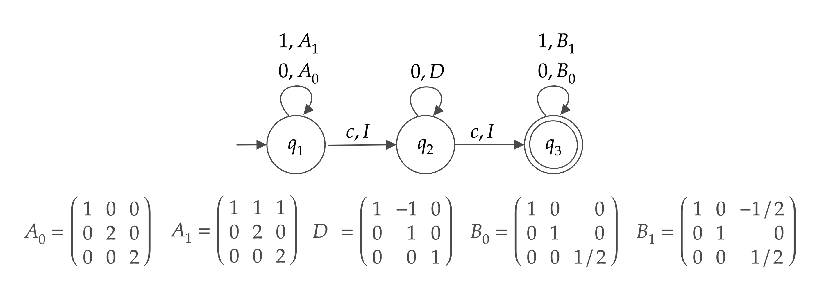
The initial vector of is . The idea is to use base-2 encoding to store in the second and the third entries of the vector with the help of the matrices and . While reading the 0 sequence, the second entry is decremented using the matrix . While reading the last sequence between two ’s, the inverses of the matrices used for base-2 encoding is used to check whether the sequence corresponds to the string . ∎
4.5 Relationship with Extended Finite Automata
In this section, we will exploit a relationship between 1NBHVA()’s and the extended finite automata over free groups to demonstrate the power of homing vector automata.
The two models seem to be linked in the case of finite automata over matrix groups, as the register is multiplied with a matrix at each step of the computation. Let us emphasize that the two models are different in the following sense. In a homing vector automaton, there is an initial vector , and the accepted strings are those which label a computation path along which the product of the sequence of matrices on the transitions is a matrix , such that . In the most general setting, the set of transition matrices belongs to the semigroup of rational matrices. In an accepting computation, the product of the matrices belongs to the stabilizer subsemigroup of the set of rational matrices with respect to . In contrast, in an extended finite automaton over a matrix group, accepting computations are those in which . In that sense, one-way nondeterministic blind homing vector automata can be seen as akin to what someone who wanted to define a version of extended finite automata associated with general matrix semigroups, rather than groups, would come up with. In fact, the homing vector automaton can be seen as a special case of the rational semigroup automaton which is defined in [69] as follows:
Let be a monoid. An -automaton is said to be with targets if it is equipped with two subsets called the initial set and the terminal set respectively. An input string is accepted by the automaton if there exists a computation from the initial state to some accepting state such that , where and is the content of the register of the machine after the reading of . In the case that and are rational subsets of , the model is called rational monoid automaton defined by [35, 69].
Rational semigroup automata are defined analogously by taking as a semigroup instead of a monoid.
Note that the family of languages accepted by rational monoid automata where coincides with the set of languages recognized by ordinary -automata. Letting where is the initial vector of a homing vector automaton and to be a semigroup of matrices, one obtains homing vector automata.
We start by looking at the case of matrices. Recall from Subsection 3.2.2 that admits a representation by matrices. In particular, the group generated by the matrices
is isomorphic to .
Using the matrix representation of , any -automaton can be simulated by a suitably defined homing vector automaton that is of dimension 2, blind, nondeterministic, and one-way. The proof is due to Flavio D’Alessandro and can be found in [16].
Theorem 4.15.
This allows us to draw the following conclusion about the class of languages recognized by 1NBHVA(2)’s.
Corollary 4.16.
The family of context-free languages is included in
In the proof of Theorem 4.15, the matrices used for the simulation of an -automaton belong to . In the following theorem, we show that 1NBHVAs are more powerful than the corresponding monoid automata, when the matrices are restricted to the monoid .
Theorem 4.17.
.
Proof.
Now we are going to prove that the inclusion is proper. Let us construct a 1NBHVA(2) recognizing the non-context-free language . The state diagram of is given in Figure 4.6.

The initial vector of is . While reading in , multiplies its vector with the matrix . It moves to when it scans the first and multiplies its vector with the matrix as it reads each . multiplies its vector with the matrix and moves to .
When the vector is multiplied by , the first entry of the vector is increased by 1 and when the vector is multiplied by , the second entry of the vector is multiplied by 2. Hence, after reading an input string of the form , the vector is equal to , as a result of the multiplication by the matrix product . After multiplication by , the second entry of the vector is subtracted from the first entry and this value is stored in both entries of the vector. The value of the final vector is equal to iff . Hence, the accepted strings are those which are of the form . ∎
For matrices, we don’t have a comparability result among the classes of languages recognized by the two models. The major limitation lies in the fact that the limits of finite automata over matrix groups are not known. Furthermore, we don’t know how to directly simulate a finite automaton overa group of matrices with a 1NBHVA(3). Nevertheless, let us note that 1NBHVA(3)s defined with matrices from can recognize any language recognized by 1NBCAs as we showed in Theorem 4.10, whereas it is an open question whether includes the class of languages recognized by 1N3BCAs.
Next we are going to demonstrate the power of 1NBHVA()s for . Recall that by Theorem 3.17. The proof idea of Theorem 3.17 is to embed two copies of into matrices. Combining this idea with the proof of Theorem 4.15, one can show that 1NBHVA(4)s recognize any recursively enumerable language. Since the computation of a 1NBHVA() involves vector matrix multiplications by computable numbers, it can be simulated by a Turing machine and it follows that any language recognized by a 1NBHVA() is recursively enumerable. The proof details are omitted here and can be found in [16].
Theorem 4.18.
for .
4.6 Real-time Homing Vector Automata
In the previous section, we have seen that allowing one-way access to the input tape raises nondeterministic blind homing vector automata of small vector dimension to Turing equivalence. For this reason, we will be focusing on real-time input in this section.
Let us start with an example. We show that by allowing nondeterminism, it is possible to recognize an -complete language in real-time and with matrices belonging to set . is the -complete language which is the collection of all strings of the form , such that and the ’s are numbers in binary notation , and there exists a set satisfying , where . We define
in which the binary numbers appear in reverse order. It is obvious that , since . It is possible to reduce to in polynomial time by reversing the binary numbers that appear in the input. Therefore, we can conclude that is -complete.
Example 4.19.
.
We construct a NBHVA(5) recognizing . The state transition diagram of recognizing is given in Figure 4.7.

The idea of this construction is to read the binary numbers in the string to entries of the vector, and to nondeterministically select the set of numbers that add up to . We let the initial vector equal . We first encode to the first entry of the vector as follows: While scanning the symbols of , multiplies the vector with the matrix (resp. ) for each scanned (resp. ). The powers of 2 required for the encoding are obtained by adding the third and fourth entries, which always contain identical numbers, to each other, creating the effect of multiplication by 2. When reads a , multiplies the vector with the matrix which subtracts the second entry from the first entry and resets the second entry back to 0, and the third and fourth entries back to 1. In the rest of the computation, nondeterministically decides which ’s to subtract from the first entry. Each selected is encoded using the same technique into the second entry of the vector. While scanning the symbols of , multiplies the vector with the matrix (resp. ) for each scanned (resp. ).
chooses another if it wishes, and the same procedure is applied. At the end of the input, accepts if the vector is equal to , which requires that the first entry of the vector is equal to 0. This is possible iff there exists a set of ’s whose sum add up to .
4.6.1 Comparisons Among the Different Versions
We start by comparing the deterministic blind and non-blind versions of our model.
Theorem 4.20.
Proof.
It is obvious that any DBHVA() can be simulated by a DHVA(). We are going to prove that the inclusion is proper by the witness language . Let us first construct a DHVA(2) recognizing . The state transition diagram of is given in Figure 4.8. The idea is to simulate a counter with the help of the matrices. Starting with the initial vector , multiplies the vector with the matrix for each it reads before the ’s, incrementing the first entry of the vector with each such multiplication. After finishing reading the first segment of ’s, multiplies the vector with the matrix , decrementing the first entry of the vector for each .

checks the current value of the vector for equality to when reading the first . If the equality is detected, it is the case that , and multiplies the vector with the identity matrix at each step for the rest of the computation. If that is not the case, continues to multiply the vector with matrix for each after the ’s. The value of the vector will be equal to at the end of the computation if and only if or .
Note that can be also recognized by a DHVA(1) by using the one-dimensional matrices and .
Now we are going to show that cannot be recognized by any DBHVA(). Suppose for a contradiction that is recognized by some DBHVA() . After reading a prefix of ’s, the computation of on a sufficiently long suffix of ’s will go through a sequence of states, followed by a state loop. Suppose that is in the same state after reading two different strings and , . Now consider the strings and . After reading any one of these strings, should be in the same accept state, and the vector should be at its initial value. Assume that the strings in question are both extended with one more . Since the same vector is being multiplied with the same matrix associated with the same state during the processing of that last , it is not possible for to give different responses to and . Noting that , whereas , we conclude that cannot be recognized by any DBHVA(). ∎
In the following theorem, we show that nondeterministic real-time homing vector automata are more powerful than their deterministic versions, both in the blind and nonblind cases.
Theorem 4.21.
- (i)
.
- (ii)
.
Proof.
A language is in class () if there is a deterministic Turing machine that decides within time and space where is the length of the input. Since the numbers in the vector can grow by at most a fixed number of bits in each multiplication, a Turing machine simulating a DHVA() requires only linear space [9]. Since the numbers in the vector can have length , whereas the matrix dimensions and entries are independent of the input length , multiplication of a vector and a matrix requires time for each input symbol. We can conclude that (DHVA()).
4.6.2 A Hierarchy Result
We will now establish a hierarchy result on real-time deterministic homing vector automata based on the dimension of the vector, when the matrix entries belong to a restricted set.
Theorem 4.22.
Then for .
Proof.
Using the generalized Stern-Brocot encoding, we showed that it is possible to recognize by a DBHVA() in Exercise 4.6.
We are now going to show that for . We first note that the value of any entry of a vector of size can be at most after reading symbols. This is possible by letting the initial vector have in all entries, and multiplying the vector with the matrix with all entries equal to at each step. Similarly, the smallest possible value of an entry is , and so the number of possible different values for a single entry is . If the machine has states, is an upper bound for the number of different reachable configurations after reading symbols. Since there are strings of length when the alphabet consists of symbols, for large and , the machine will end up in the same configuration after reading two different strings and . This will cause the strings and which are not in to be accepted by the machine. Therefore, we conclude that .
Since a vector automaton with a larger vector size can trivially simulate a vector automaton with a smaller vector size, this result applies to our case. ∎
4.6.3 Closure Properties
In this section, we examine the closure properties of the class of languages recognized by real-time homing vector automata. We start with a lemma which will be useful in our proofs. The languages mentioned below are from [6].
Lemma 4.23.
- (i)
.
- (ii)
.
- (iii)
.
- (iv)
.
Proof.
We can show all these languages to be unrecognizable by DHVAs by applying the following common reasoning. Assume that the language in question is recognized by some DHVA() . Since there are finitely many states, one of the states of will end up accepting more than one member of the language. For each language, we will focus on two such members and . Note that is in the same configuration (since it has also returned to its initial vector) after reading both and . We then append another string to both strings, selected so that and . The responses of to the and has to be identical, since it will have returned to the same configuration after processing both strings. We conclude that cannot distinguish between these two strings, and therefore that . All that remains is to provide the strings , , and for the languages in the statement of the lemma. In the following, and .
- (i)
, , and .
- (ii)
, and .
- (iii)
, , and for .
- (iv)
, , and .
∎
Let us note that it is possible to recognize the languages mentioned in the proofs with DHVA()’s of smaller vector size when the vector entries are not restricted to be integers.
Theorem 4.24.
- (i)
is closed under the following operations:
- (a)
intersection with a regular set
- (a)
- (ii)
is not closed under the following operations:
- (a)
union
- (b)
concatenation
- (c)
intersection
- (d)
star
- (e)
homomorphism
- (f)
reversal
- (g)
complementation
- (a)
Proof.
- (i)
- (a)
Let be recognized by a DHVA() and be a language recognized by a finite state automaton . Let us construct a DHVA() recognizing . keeps track of the vector and the current state of as well as the current state of Let be the state set of and . For each , and , where and . is the pair and is the set of pairs of states where both of the states are accept states of or . We obtain a DHVA() recognizing .
- (a)
- (ii)
- (a)
Let and . and can be recognized by a DBHVA(2) which simulates a deterministic blind one-counter automaton whereas cannot be recognized by any DHVA() for any by Lemma 4.23.
- (b)
For the languages and , , which cannot be recognized by any DHVA() for any by Lemma 4.23 and Part i.a) of this theorem.
- (c)
Let and . Both and can be recognized by DHVA(2)s which simulate deterministic one-counter automata, whereas cannot be recognized by any DHVA() for any by Lemma 4.23.
- (d)
Let . A DBHVA() recognizing branches into one of two computation paths depending on the first scanned symbol . If , simulates a deterministic blind one-counter automaton recognizing and if , simulates a deterministic blind one-counter automaton recognizing . Now suppose . Then . A DHVA() recognizing can be easily modified to obtain a DHVA() recognizing the language , which is not in by Lemma 4.23.
- (e)
Let . A DBHVA() recognizing works similarly to the one in part d). Now consider the homomorphism such that , and . , which cannot be recognized by any DHVA() for any by Lemma 4.23.
- (f)
Let . A DBHVA() recognizing works similarly to the one in part d). Now consider the reverse of , , which cannot be recognized by any DHVA() for any by Lemma 4.23.
- (g)
Consider , which can be recognized by a DHVA(3). cannot be recognized by any DHVA() by Lemma 4.23.
- (a)
∎
The set of languages recognized by real-time nondeterministic homing vector automata is closed under union, star and concatenation The constructions are fairly simple and omitted.
Theorem 4.25.
- (i)
is closed under the following operations:
- (a)
intersection
- (a)
- (ii)
is not closed under the following operations:
- (a)
union
- (b)
concatenation
- (c)
star
- (d)
homomorphism
- (e)
reversal
- (f)
complementation
- (a)
Proof.
- (i)
- (a)
Let and be recognized by DBHVA() and DBHVA() , respectively. Let us construct a DBHVA() recognizing where . Let be the state set of and . For each and , , where , and is a block diagonal matrix with and on its diagonal. is the pair , and is the set of pairs of states where both of the states are accept states of or . The initial vector of is of the form and has dimension . keeps track of the current states and the current values of both vectors by simultaneously multiplying its vector with the appropriate matrices. Since the computation is blind, the value of the vector is checked only at the end of the computation, and an input string is accepted if the vector is equal to its initial value.
- (a)
- (ii)
The proofs for the non-blind version also apply here. The proof for part (f) follows from the fact that is closed under intersection but not union.
∎
The set of languages recognized by real-time nondeterministic blind homing vector automata is closed under union and intersection. The construction for union is straightforward, and the construction for intersection is identical to the deterministic case.
4.6.4 Stateless computation
Given two strings, a finite automaton is said to separate them if it accepts one and rejects the other. Introduced by Goralčík and Koubek [70], the string separation problem asks for the minimum number of states needed for accomplishing this task. String separation by homing vector automata and vector automata have been investigated in [17]. It turns out that a homing vector automaton needs at least two states to separate any pair of strings, regardless of the dimension of the vector. We are therefore motivated to examine the limitations imposed by statelessness on homing vector automata in more detail.
Stateless machines [71, 72, 73] have been investigated by many researchers, motivated by their relation to membrane computing and P systems [74], which are stateless models inspired from biology. While vector automata can simulate their classical states in their vectors by using longer vectors, this is not the case for homing vector automata.
Our study on stateless homing vector automata yields a characterization for the class of languages recognized by stateless real-time deterministic FAMs without equality (0-DFAMW) [6]. It turns out that a language is recognized by a 0-DFAMW iff it is commutative and its Parikh image is the set of nonnegative solutions to a system of linear homogeneous Diophantine equations. When the computation is nondeterministic, then any language recognized by a stateless real-time nondeterministic FAM without equality is commutative. We conclude by providing some further examples and observations about language recognition power of stateless homing vector automata.
4.6.4.1 Observations
The limitation of having a single state for homing vector automata leads to the acceptance of the string , whenever the string is accepted. This is true since further repetition of the same input naturally carries the vector through a trajectory that ends up in its initial value. Based on this observation, we can list the following consequences:
For ,
- •
If string is accepted by a 0-XHVA , then any member of is also accepted by .
- •
If all members of a language are accepted by a 0-XHVA , then any string in is also accepted by .
- •
If language is recognized by a 0-XHVA, then .
- •
0-XHVAs cannot recognize any finite language except .
We can further make the following observation for deterministic models.
Lemma 4.26.
If the strings and are accepted by a 0-XHVA where , then the string is also accepted by .
Proof.
After reading , the value of the vector is equal to its initial value. Since is also accepted by , reading results in acceptance when started with the initial vector. ∎
For the unary case we have the following.
Theorem 4.27.
If the strings and () are accepted by a 0-XHVA where , then the string is also accepted by .
Proof.
It is well known that for any positive integers , there are two integers and such that . Assume that is positive and is non-positive. (The other case is symmetric.) Note that . The strings and are accepted by . By Lemma 4.26, the string , which is , is also accepted by .
∎
Corollary 4.28.
If the strings and () are accepted by a 0-XHVA where and , then recognizes .
Let us now investigate the case where the set of matrices is commutative.
Let be a language. The commutative closure of is defined as . A language is commutative if .
Theorem 4.29.
If a language is recognized by a 0-XBHVA where with a commutative set of matrices, then is commutative.
Proof.
Let and suppose that the string is accepted by . Let be the product of the matrices labeling the computation such that
where is the initial vector of . Since the matrices are commutative, then for any permutation ,
This leads to the acceptance of the string since
Hence, if is accepted by , then any string obtained from by permuting its letters is also accepted by . Any string with is in and we conclude that is commutative. ∎
When the computation is not blind, then the class of languages recognized is no longer commutative. The language of balanced strings of brackets can be recognized by 0-DHVA(1) as follows. Starting with the initial vector , for each left bracket the vector is multiplied by . As long as the vector is not equal to (1), for each right bracket, the vector is multiplied by (). If the vector is equal to and the next symbol is a right bracket, then the vector is set to (0).
Corollary 4.30.
If a language is recognized by a 0-XBHVA where with a commutative set of matrices, then .
Proof.
Suppose that . Then it is clear that will be also accepted by by Theorem 4.29 and . Since for every string it is true that if and only if , we conclude that . ∎
4.6.4.2 Regular languages
Let be an -state deterministic finite automaton. Without loss of generality, we can enumerate its states as where is the initial state. Moreover we can denote by , which is the basis vector in dimension having 1 in its ’th entry, and 0 otherwise. Besides, for each symbol , we can design a zero-one matrix, say , that represents the transitions between the states, i.e. if and only if switches from to when reading symbol . Thus, the computation of on an input, say , can be traced by matrix-vector multiplication:
if and only if ends its computation in after reading .
Based on this representation, we can easily observe that if a language is recognized by an -DFA whose initial state is the single accept state, then is recognized by a 0-DBHVA().
Let us give some examples of stateless HVAs recognizing regular languages.
Example 4.31.
For , .
Let us construct a 0-DBHVA(2) recognizing . The initial vector of is . For each , the value in the ’th entry of the vector is transferred to the ’st entry when , and, the rest of the entries are set to 0. For each , the value in the ’th entry of the vector is transferred to the ’th entry, and the rest of the entries are set to 0, (). Thus, we return to the initial vector if and only if after some number of blocks have been read.
Example 4.32.
.
It is easy to observe that any unary -state DFA whose initial state is the single accept state can recognize either or for some . Hence, for any , the language is recognized by a 0-DBHVA().
Note that if it is allowed to use arbitrary algebraic numbers in the transition matrices, then for every , the language is recognized by a 0-DBHVA(2) with initial vector that multiplies its vector with the matrix
for each scanned symbol. (The entries of are algebraic for any [75].)
One may ask whether all regular languages satisfying can be recognized by stateless HVAs. We provide a negative answer for the deterministic model. The language is defined as , satisfying that . cannot be recognized by any 0-DHVA since a 0-DHVA which accepts and , also accepts by Lemma 4.26.
4.6.4.3 Stateless 1-dimensional HVAs
We now focus on stateless HVAs whose vectors have dimension 1 and demonstrate some results on stateless FAMWs. Note that stateless FAMs do not process the end-marker by definition, since their single state is also an accept state and the computation ends once is scanned in an accept state.
We start by comparing the class of languages recognized by stateless versions of BCAs, FAMWs, and BHVA(1)s. The equivalence between BCA and FAMWs and BHVA(1)s does not hold immediately in the stateless case. The reason is that the counters can only be updated by the set in a single step since additional states are needed to update the counters by arbitrary integers (see Fact 2.1). Furthermore, the capability of multiplication with negative rational numbers brings additional power to the stateless DBHVA(1)s.
Theorem 4.33.
where .
Proof.
Let . The following 0-DBHVA(1) recognizes : The register is multiplied by and when the machine reads an and respectively.
Suppose that there exists some 0-XFAMW recognizing . Let and be the positive rational numbers that are multiplied by the register upon reading and . Since , it is true that . Since both and are positive, it is not possible that . It follows that , in which case the string is accepted and we get a contradiction. Hence we conclude that cannot be recognized by any 0-XFAMW. ∎
When the register is multiplied with only positive rational numbers, then we have (0-XFAMW)=(0-XBHVA(1)).
For real-time and blind machines, we can state the following result.
Corollary 4.34.
If where , then is commutative.
Proof.
Let us recall Fact 2.3, which states that a bounded language is accepted by a 1NFAMW iff it is semilinear [6]. In the next theorem, we prove a similar result and characterize the class of languages recognized by 0-DFAMWs. We show that any language recognized by a 0-DFAMW is commutative and semilinear. Furthermore, any commutative language whose Parikh image is the set of nonnegative solutions to a system of linear homogenous Diophantine equations can be recognized by a 0-DFAMW.
Theorem 4.35.
iff is commutative and is the set of nonnegative integer solutions to a system of linear homogeneous Diophantine equations.
Proof.
Let be a language over the alphabet recognized by a 0-DFAMW . Let be the set of rational numbers such that the register is multiplied with upon reading . Let be the set of prime factors of the denominators and the numerators of the rational numbers in . Then each can be expressed as
If a string is accepted by , then the value of the register should be equal to 1 after reading , which is possible only if
This leads to the following system of linear Diophantine equations in variables.
For , the ’th equation is stating that the exponent of is equal to 0 after reading .
Hence, we can conclude that the Parikh images of the accepted strings are the nonnegative solutions to a system of linear homogeneous Diophantine equations. is commutative by Theorem 4.34. (One can further conclude that is semilinear.)
For the converse, suppose that we are given a commutative language over the alphabet . Let be the set of Parikh images of the strings in . is the set of nonnegative solutions to a system of, say, linear homogeneous Diophantine equations in unknowns,
where .
We construct a 0-DFAMW recognizing as follows. We choose a set of distinct prime numbers, . When reads , the register is multiplied by
Suppose that a string is accepted by . Then
The product is equal to 1 if all of the exponents of the prime factors are equal to 0, that is when . Hence we see that the set of accepted strings are those with Parikh image in . Since is commutative, any string with belongs to and we conclude that recognizes .
∎
Note that (0-DFAMW)=(0-1DFAMW), since a 0-1DFAMW that has an instruction to stay on some input symbol cannot read the rest of the string. The reasoning of Lemma 4.8 applies.
4.6.4.4 Additional Results on Stateless Homing Vector Automata
One sees that the nonregular language cannot be recognized by any 0-NHVA() for any , since . On the other hand, can be recognized by a 0-DBHVA(1) with initial vector , and transition matrices and . It is possible to recognize the star of , even in the deterministic and blind computation mode with a stateless homing vector automaton. Note that cannot be recognized by any 1NFAMW [6]. The proof is due to Abuzer Yakaryılmaz and can be found in [17].
Theorem 4.36.
The language is recognized by a 0-DBHVA(10).
Nondeterministic HVAs are more powerful than their deterministic variants in terms of language recognition in general. In the next theorem, we show that this is also true for the stateless models.
Theorem 4.37.
- (i)
- (ii)
Proof.
Let us construct a 0-NBHVA(1) recognizing . Starting with the initial vector , multiplies its vector with for each and with or for each nondeterministically.
Suppose that can be recognized by a 0-DHVA() . The strings and are accepted by . By Lemma 4.26, the string is also accepted by . We obtain a contradiction, and conclude that cannot be recognized by any 0-DHVA(). ∎
Now let us compare the language recognition power of 1 and 2 dimensional stateless HVAs.
Theorem 4.38.
- (i)
- (ii)
Proof.
Now, we compare the blind and non-blind versions of one dimensional HVAs.
Theorem 4.39.
- (i)
- (ii)
Proof.
Let us construct a 0-DHVA(1) recognizing . The initial vector is equal to (1). For each scanned , multiplies its vector with if it is equal to its initial value, and with otherwise. For each scanned , multiplies its vector with if it is equal to its initial value, and with otherwise. cannot be recognized by any 0-NBHVA(1) as we saw in the proof of Theorem 4.38. ∎
Let us look at some closure properties for the stateless models. All of the classes associated with the stateless models are closed under the star operation since for any language recognized by a stateless homing vector automaton, it is true that .
Theorem 4.40.
- (i)
is closed under the following operation:
- (a)
intersection
- (a)
- (ii)
and are not closed under the following operations:
- (a)
union
- (b)
complement
- (c)
concatenation
- (a)
Proof.
- (i)
- (a)
The proof of Theorem 4.25 that is closed under intersection is also valid for stateless models.
- (a)
- (ii)
- (a)
- (b)
The complement of the language ()is not recognized by any 0-NHVA(), since contains and any 0-NHVA() accepting accepts any member of .
- (c)
The concatenation of and , , cannot be recognized by any 0-DHVA.
∎
and are not closed under complement. is closed under intersection. The proofs are identical.
4.7 Open Questions
What can we say about the relationship between real-time homing vector automata and one-way homing vector automata? We conjecture that one-way nondeterministic blind homing vector automata are more powerful than their real-time versions. Our candidate language is , which can be recognized by a 1NBHVA(2). Note that when the machine in consideration is deterministic and blind, the real-time and one-way versions are equivalent in power.
Can we show a separation result between the class of languages recognized based on the set of matrices used during the transitions of a homing vector automaton?
Can we show a hierarchy result between the classes of languages recognized by deterministic homing vector automata of dimensions and for some , maybe when the matrix entries are restricted to the set ? Consider the family of languages . We conjecture that it is not possible to recognize with a homing vector automaton of dimension less than with the restricted set of matrices.
Let be a group of matrices. Can we always construct a recognizing the same language as a given -automaton? (Note that we have proven that this is the case for and -automaton.)
Suppose that one can always find a suitable initial vector such that for every except the identity matrix, . Then one could construct the required from the given -automaton directly. For which groups is it always possible to find such a vector?
What can we say about the reverse direction? For instance, is every language recognized by some context-free?
We proved that 1NBHVA()s are more powerful than extended finite automata when both are defined over integer matrices. Is this result still true when both models are defined over integer matrices?
Do 0-NHVA()s recognize every regular language satisfying ? Is there any nonregular language satisfying that cannot be recognized by any stateless HVA?
We proved that any language recognized by a 0-NFAMW is commutative. What can we say about the non-blind case?
We gave a characterization for the class of languages recognized by 0-DFAMWs. Can we give a similar characterization for the non-blind and nondeterministic models?
Chapter 5 VALENCE GRAMMARS AND VALENCE AUTOMATA
In this chapter, we are going to focus on context-free valence grammars, valence automata and valence pushdown automata.
We start by stating the formal definitions in Section 5.1. In Section 5.2, we show that valence pushdown automata and finite valence automata are equivalent in terms of language recognition power, using the well known equivalence between pushdown automata and finite automata over polycyclic monoids. Then, we extend some results proven for valence automata in [35] to context-free valence grammars and give the properties of the set of languages generated by context-free valence grammars in Section 5.3. We state some open questions in Section 5.4.
5.1 Definitions
Let be a context-free grammar where is the set of variables, is the terminal alphabet, is the set of rules or productions, and is the start symbol. We will denote by and the step derivation relation and its regular closure respectively. denotes the language of words generated by .
Given a monoid , a context-free valence grammar over [8] is a five-tuple , where are defined as before and is a finite set of objects called valence rules. Every valence rule can be thus described as an ordered pair , where and . The element is called the valence of .
The step derivation of the valence grammar is defined as follows: if there exists a valence rule such that and and . The regular closure of will be denoted by . A derivation of will be said successful or valid if it is of the form , that is, it transforms the pair into the pair , after finitely many applications of the step derivation relation. The language generated by is the set of all the words of such that .
A context-free valence grammar is said to be regular if all of its rules are right-linear, that is, every valence rule is such that where and . The language families generated by context-free and regular valence grammars over are denoted by and , respectively.
Let be a one-way nondeterministic pushdown automaton. Given a monoid , the nondeterministic valence pushdown automaton (valence PDA) over is the model of computation obtained from as follows: with every transition of is assigned an element of , called the valence of the transition. Then the valence of an arbitrary computation is defined as the product of the valences of all the transitions of the computation (taken in the obvious order). A word of is said to be accepted by the model if there exists an accepting computation for the word whose valence is the identity of . The set of all the accepted words is defined as the language accepted by the valence pushdown automaton. The family of languages accepted by valence PDA over is denoted . It is worth noticing that the equivalence between valence pushdown automata and valence context-free grammars does not hold for an arbitrary monoid. However a result of [8] shows that the equivalence is true if is a commutative monoid.
In the case that pushdown automaton is a finite state automaton, the corresponding valence model is called the valence automaton over . This model coincides with the -automaton, and the family of languages accepted by valence automata is exactly . The equivalence between valence automata and regular valence grammars is proven in [8].
Introduced by [7], the valence grammars have been studied by various authors including [76, 77, 8]. A through study of several remarkable structural properties of the languages generated by the corresponding valence grammars has been done in [8], over arbitrary monoids and in particular over commutative groups. In [8], the following fact is proven.
Fact 5.1.
[8] Context-free valence grammars over finite or commutative monoids are not stronger than context-free valence grammars over finite or commutative groups.
It is left open in [8] whether context-free grammars with valences from finite monoids are more powerful than ordinary context-free grammars and the question is answered in [78].
Fact 5.2.
[78] Context-free grammars over finite monoids recognize exactly the class of context-free languages.
Now we are going to present some definitions about monoids and semigroups.
Let be a semigroup. Given subsets and of semigroups , is the set . An ideal of a semigroup is a subset of with the property that .
The binary relation defined by
is a congruence. The equivalence classes of are itself and every one-element set with . The quotient semigroup is written as and is called the Rees quotient semigroup [79].
A semigroup is called simple if it contains no proper ideal. A semigroup with a zero element is called 0- if the only ideals of are and itself, and .
5.2 Equivalence of Finite and Pushdown Automata with Valences
In this section, we are going to prove that valence pushdown automata are only as powerful as valence automata.
Let us recall the definition of polycyclic monoid which we have introduced in Subsection 3.3.3. Let be a finite alphabet and let be the free monoid of words over . For each symbol , let and be functions from into defined as follows: for every ,
The monoid of all partial functions on generated by the set of functions is called the polycyclic monoid on . We will focus on the polycyclic monoid of rank 2, which will be denoted by , since it contains every polycyclic monoid of countable rank.
Theorem 5.3.
For any monoid , .
Proof.
Let and be a valence PDA recognizing . We know that a PDA with stack alphabet is equivalent to a valence automaton over . Hence, can be seen as an NFA where two distinct valences (one in and one in ) are assigned to each transition. An equivalent valence automaton can be constructed, where a valence from the monoid is assigned to each transition. Recall that the partial functions and model the operations of popping and pushing respectively. A transition of of the form where , , and can be expressed equivalently as where .
A string is accepted by if and only if the product of the valences labeling the transitions in is equal to , equivalently when the product of the valences labeling the transitions in is equal to the identity element of and the stack is empty. Since any polycyclic monoid is embedded in , we conclude that .
Conversely, let and let be a valence automaton over recognizing . Suppose that is a valence labeling a transition of . The product of the labels of a computation which involves a transition labeled by the zero element of cannot be equal to the identity element. Hence we can remove such transitions. Any nonzero element of can be written as
for some and , after canceling out elements of the form and , where is the generator set for . The product can be interpreted as a series of pop operations followed by a series of push operations performed by a PDA, without consuming any input symbol. Hence, an equivalent valence PDA can be constructed where a valence from is assigned to each transition. Let where , , and be a transition in . In , we need additional states and the following transitions to mimic that specific transition of .
A string is accepted by if and only if the product of the valences labeling the transitions in is equal to the identity element of and the stack is empty, equivalently when the product of the valences labeling the transitions in is equal to . We conclude that . ∎
Note that when is commutative, the equality also holds.
Corollary 5.4.
Let be a polycyclic monoid of rank 2 or more. Then is the class of recursively enumerable languages.
5.3 Context-free Valence Languages
It is known that the class of languages generated by regular valence grammars and the class of languages recognized by valence automata coincide [8]. In this section, we are going to prove that the results proven in [35] which hold for valence automata and therefore regular valence grammars, also hold for context-free valence grammars. Although the proofs are almost identical, they are presented here for completeness. Note that the same proofs can be also adapted to valence PDA.
In [35] Proposition 4.1.1, it is shown that the elements belonging to a proper ideal of a monoid do not have any use in the corresponding monoid automaton. We show that the same result holds for context-free valence grammars.
Proposition 5.5.
Let be a proper ideal of a monoid . Then
Proof.
Let and let be a context-free valence grammar over the monoid such that . The product of the valences which appear in a derivation containing a rule with valence , will itself belong to . Since is a proper ideal and , such a derivation is not valid. Hence any such rules can be removed from the grammar and we can assume that has no such rules. For any , it follows that in if and only if in . Let be the context-free grammar with valences in , obtained from by replacing each valence with . It follows that a string has a valid derivation in if and only if the product of the valences is mapped to in . Hence .
Conversely let and let be a context-free grammar over the monoid such that . Suppose that there exists a valid derivation consisting of a rule with as the valence. Then the product of the valences of the whole derivation will be , which is not possible. Let be the context-free grammar with valences in , obtained from by replacing each valence with . Since in if and only if in , a string has a valid derivation in if and only if the product of the valences is mapped to in . Hence . ∎
Let be a semigroup. is the null semigroup if it has an absorbing element zero and if the product of any two elements in is equal to zero. A null semigroup with two elements is denoted by .
The following corollary is analogous to [35] Cor. 4.1.2.
Corollary 5.6.
For every monoid , there is a simple or 0-simple monoid such that .
Proof.
If has no proper ideals then it is simple. Otherwise, let be the union of all proper ideals of and let . We can conclude from the proof of Cor. 4.1.2 [35] that or is 0-simple. If , then is and the semigroup does not add any power to the grammar since it does not even contain the identity element. Hence, where is the trivial monoid which is simple. In the latter case is 0-simple and by Proposition 5.5, . ∎
Proposition 4.1.3 of [35] states that a finite automaton over a monoid with a zero element is no more powerful then a finite automaton over a version of the same monoid from which the zero element has been removed, in terms of language recognition. The result is still true for context-free valence grammars since the same proof idea applies. The following notation is used: if has no zero element and otherwise.
Proposition 5.7.
Let be a monoid. Then .
Proof.
Since , it follows that . Suppose and let be a context-free valence grammar with valences in and . Note that a valid derivation cannot contain a rule with a zero valence since otherwise the product of the valences would be equal to zero. Any such rules can be removed from to obtain , a context-free grammar with valences in , without changing the language, and . ∎
In the case , the monoid coincides with the well-known structure of bicyclic monoid which will be denoted by B.
Fact 5.8.
[35] A simple (0-simple) monoid with identity is either a group (respectively, a group with 0 adjoined) or contains a copy of the bicyclic monoid as a submonoid having 1 as its identity element.
Theorem 5.9.
Let be a monoid. Then either for some group , or .
Proof.
Let be a monoid. By Corollary 5.6, then for some simple or 0-simple monoid. By Fact 5.8, is either a group (or a group with zero adjoined) or contains a copy of the bicyclic monoid. If is a group, then the result follows. If is a group with zero adjoined, then by 5.7, for some group . Otherwise, it should be the case that . ∎
Now we are ready to prove the main theorem of the section which will allow us to determine the properties of the set of languages generated by context-free valence grammars. We need the following proposition which is the grammar analogue of Proposition 1 of [37].
Proposition 5.10.
Let be a monoid, and suppose that is accepted by a context-free valence grammar over . Then there exists a finitely generated submonoid of such that is accepted by a context-free valence grammar over .
Proof.
There are only finitely many valences appearing in the rules of a grammar since the set of rules of a grammar is finite. Hence, the valences appearing in derivations are from the submonoid of generated by those elements. So the grammar can be viewed as a context-free valence grammar over . ∎
Recall that a group is locally finite if every finitely generated subgroup of is finite and periodic if every element of the group has finite order.
Theorem 5.11.
Let be a monoid. Then either
- (i)
equals ,
- (ii)
contains ,
- (iii)
contains or
- (iv)
is equal to for an infinite periodic group which is not locally finite.
Proof.
Let be a monoid. Then either for some group , or . Then in the former case holds. In the latter case for some group .
In the latter case, if is a group with zero adjoined, then by Proposition 5.7 we know that for some group . If is not periodic, then it has an element of infinite order which generates a subgroup isomorphic to and hence (iii) follows. Otherwise, suppose that is locally finite. By Proposition 5.10, every language in belongs to for some finitely generated subgroup of . Since is locally finite, is finite. Any language is context-free by a result from [78] and hence holds. The only remaining case is that is a periodic group which is not locally finite, in which case holds. ∎
The result about valence grammars over commutative monoids which we have stated in Fact 5.1, now follows as a corollary of Theorem 5.11.
Corollary 5.12.
Let be a commutative monoid. Then for some group .
Proof.
Since no commutative monoid can contain a copy of the bicyclic monoid as a submonoid, the result follows by the proof of Theorem 5.11. ∎
5.4 Open Questions
We proved that a valence PDA over is equivalent to a valence automaton over . Can we prove a similar equivalence result for context-free valence grammars?
In Theorem 5.11, we conclude that contains the class when is a monoid that contains B. Since B is not commutative, no correspondence with valence PDA exists, and little is known about the class , except that it contains the set of partially blind one counter languages. What can we say further about ?
Chapter 6 CONCLUSION
The main purpose of this thesis is to explore various computational models with storage. We mainly examine extended finite automata and homing vector automata, investigating the language recognition power of these models under different restrictions. We also present several results about valence pushdown automata and context-free valence grammars.
Matrices have a fundamental role in this study. Focusing on finite automata over matrix groups, both models can be regarded as a finite automaton equipped with a storage mechanism that is modified through matrix multiplications.
We first examine the class of languages recognized by finite automata over rational and integer matrix groups and compare them with the previously known language classes. Our findings can be summarized as follows:
- •
Finite automata over the group of integer matrices recognize exactly the class of context-free languages.
- •
Finite automata over the group of rational matrices with determinant 1 can recognize some non-context-free languages.
Together with the previous results, the overall picture is given in Figure 6.1. The question mark indicates that the existence of a language in the particular subset is unknown.

Next we analyze the language recognition power of extended finite automata under time restriction. We prove that the growth rate of the group is effective in the language recognition power of the corresponding group automaton, when a time bound is imposed on the machine. Using this result we prove that there exists a context-free language which cannot be recognized by any -automata in polynomial time if the group has polynomial growth. Furthermore, we investigate the class of languages recognized by group automata in linear-time and obtain the following results:
- •
Free group automata recognize exactly the class of context-free languages in linear time.
- •
Heisenberg group automata cannot recognize some context-free languages in linear time.
- •
The class of languages recognized by finite automata over the group of integer matrices is a proper superclass of the class of languages recognized by Heisenberg group automata under the restriction of linear time.
We investigate the link between the decidability problems for matrix groups and the corresponding group automata. We provide alternative proofs for the decidability of the subsemigroup membership problem for the group of integer matrices and the identity problem for the monoid of matrices with integer entries. We also prove the undecidability of the emptiness problem for finite automata over integer matrix groups.
Another way we focus on matrices is through the study of the homing vector automaton model, a finite automaton equipped with a vector. Like in many classical models where the acceptance condition is ending with the initial register value, a string is accepted by a homing vector automaton if the vector is equal to its initial value after a series of multiplications with some rational valued matrices. We define different variants of the machine such as real-time, one-way, deterministic, nondeterministic, blind, and non-blind and we add further restrictions on the machine by restricting the matrices multiplied with the register to a specific set. We investigate the relationship between homing vector automata and counter automata, proving that one-dimensional homing vector automata are equivalent to blind counter automata and the two models are incomparable when the computation is not blind. One-way nondeterministic blind homing vector automata are closely linked to extended finite automata over matrix groups and this link extends our knowledge on homing vector automata. We visualize our findings in Figure 6.2 and summarize our findings as follows:
- •
The class of languages recognized by one-way nondeterministic blind homing vector automata over the group of integer matrices with determinant 1 contains the class of context-free languages.
- •
Over the monoid of integer matrices, the class of languages recognized by one-way nondeterministic blind homing vector automata is a proper superset of the class of languages recognized by extended finite automata.
- •
Over the monoid of integer matrices, the class of languages recognized by one-way nondeterministic blind homing vector automata is a proper superset of the class of languages recognized by one-way nondeterministic blind counter automata.
- •
The class of languages recognized by one-way nondeterministic blind homing vector automata over the group of integer matrices with determinant 1 is the class of recursively enumerable languages.

We propose a new method called the generalized Stern-Brocot encoding, which enables encoding any string over an alphabet of size into a -dimensional vector. The encoding can be carried out in real-time with matrices whose entries belong to the set . We further explore real-time homing vector automata, by establishing some separation results among the various variants and discussing some closure properties. We prove that any unary language recognized by a real-time deterministic homing vector automaton is regular. Continuing our study on real-time homing vector automata, we investigate their stateless versions. We examine the language recognition power of different versions of these machines and make some observations. Our study of the stateless real-time deterministic blind one-dimensional homing vector automata yields the following characterization for the class of languages recognized by stateless deterministic finite automata with multiplication without equality.
- •
A language is recognized by a stateless deterministic finite automata with multiplication without equality iff it is commutative and its Parikh image is the set of nonnegative integer solutions to a system of linear homogeneous Diophantine equations.
Finally we look at the problem of string separation by homing vector automata and vector automata, observing that these models can separate any pair of words by using 2-dimensional vectors in the real-time, deterministic and blind computation mode.
Other computational models we investigate are the valence pushdown automata and context-free valence grammars. We prove that valence pushdown automata are equivalent to valence automata defined over some specific monoid. We generalize some results proven in the context of extended finite automata to context-free valence grammars.
To conclude, this research opens up a new perspective for analyzing the decision problems of matrix groups and various automaton models, and any computational model than can be traced by matrix multiplications. The study of extended finite automata over matrix groups and under time restriction contributes to the current literature on the topic. The classes of languages recognized by extended finite automata and homing vector automata over integer matrices of dimensions 2, 3, and 4 provides a different point of view for classifying languages.
Many questions in need of further investigation are presented throughout the thesis. The future research on the subject should concentrate on the language recognition power of extended finite automata and homing vector automata over integer matrices. We conjecture that these classes are the proper subsets of the class of recursively enumerable languages. Note that for the group of integer matrices, the decidability of the membership problem is also open.
REFERENCES
- 1. Sipser, M., Introduction to the Theory of Computation, 2nd edition, Thomson Course Technology, United States of America, 2006.
- 2. Chomsky, N., “Context-free grammars and pushdown storage”, M. I. T. Res. Lab. Electron. Quart. Prog. Report., Vol. 65, pp. 187–194, 1962.
- 3. Fischer, P. C., A. R. Meyer and A. L. Rosenberg, “Real time counter machines”, Proceedings of the 8th Annual Symposium on Switching and Automata Theory, SWAT’67 (FOCS), pp. 148–154, 1967.
- 4. Turing, A. M., “On computable numbers, with an application to the Entscheidungsproblem”, Proceedings of the London mathematical society, Vol. 2, No. 1, pp. 230–265, 1937.
- 5. Mitrana, V. and R. Stiebe, “The accepting power of finite automata over groups”, New Trends in Formal Languages, pp. 39–48, Springer-Verlag, 1997.
- 6. Ibarra, O. H., S. K. Sahni and C. E. Kim, “Finite automata with multiplication”, Theoretical Computer Science, Vol. 2, No. 3, pp. 271 – 294, 1976.
- 7. Păun, G., “A new generative device: valence grammars”, Rev. Roumaine Math. Pures Appl, Vol. 25, No. 6, pp. 911–924, 1980.
- 8. Fernau, H. and R. Stiebe, “Sequential grammars and automata with valences”, Theoretical Computer Science, Vol. 276, No. 1–2, pp. 377 – 405, 2002.
- 9. Salehi, Ö., A. Yakaryılmaz and A. C. C. Say, “Real-time vector automata”, Proceedings of the 19th International Conference on Fundamentals of Computation Theory, FCT’13, Vol. 8070 of LNCS, pp. 293–304, Springer, 2013.
- 10. Salehi, Ö., F. D’Alessandro and A. C. C. Say, “Language classes associated with automata over matrix groups”, Proceedings of the Eighth Workshop on Non-Classical Models of Automata and Applications, NCMA’16, Vol. 321 of books@ocg.at, pp. 287–300, Österreichische Computer Gesellschaft, 2016.
- 11. Salehi, Ö., F. D’Alessandro and A. C. Say, “Language classes associated with automata over matrix groups”, RAIRO-Theoretical Informatics and Applications, Vol. 52, No. 2-3-4, pp. 253–268, 2018.
- 12. Salehi, Ö. and A. C. C. Say, “Extended finite automata and decision problems for matrix semigroups.”, Tenth Workshop on Non-Classical Models of Automata and Applications (Short Papers), Vol. 321, pp. 45–52, Österreichische Computer Gesellschaft, 2018.
- 13. Turakainen, P., “Generalized automata and stochastic languages”, Proceedings of the American Mathematical Society, Vol. 21, pp. 303–309, 1969.
- 14. Lipton, R. J. and K. W. Regan, Quantum Algorithms via Linear Algebra, MIT Press, 2014.
- 15. Salehi, Ö. and A. C. C. Say, “Homing vector automata”, Proceedings of the Seventh Workshop on Non-Classical Models of Automata and Applications, NCMA’15, Vol. 318 of books@ocg.at, pp. 193–205, Österreichische Computer Gesellschaft, 2015.
- 16. Salehi, Ö., A. C. C. Say and F. D’Alessandro, “Homing vector automata”, RAIRO - Theoretical Informatics and Applications, Vol. 50, No. 4, pp. 371–386, 2016.
- 17. Salehi, Ö., A. Yakaryılmaz and A. C. C. Say, “New results on vector automata and homing vector automata”, International Journal of Foundations of Computer Science, 2019, accepted.
- 18. Salehi, Ö., F. D’Alessandro and A. C. C. Say, “Generalized results on monoids as memory”, Proceedings of the 15th International Conference on Automata and Formal Languages,AFL’17, Vol. 252 of EPTCS, pp. 234–247, 2017.
- 19. Minsky, M., Recursive Unsolvability of Post’s Problem of “tag”: And Other Topics in Theory of Truing Machines, Massachusetts Institute of Technology, Lincoln Laboratory, 1960.
- 20. Fischer, P. C., A. R. Meyer and A. L. Rosenberg, “Counter machines and counter languages”, Mathematical Systems Theory, Vol. 2, No. 3, pp. 265–283, 1968.
- 21. Greibach, S. A., “Remarks on the complexity of nondeterministic counter languages”, Theoretical Computer Science, Vol. 1, No. 4, pp. 269 – 288, 1976.
- 22. Petersen, H., “Simulations by time-bounded counter machines”, International Journal of Foundations of Computer Science, Vol. 22, pp. 395–409, 2011.
- 23. Greibach, S. A., “Remarks on blind and partially blind one-way multicounter machines”, Theoretical Computer Science, Vol. 7, pp. 311–324, 1978.
- 24. Fraleigh, J. and V. Katz, A First Course in Abstract Algebra, Addison-Wesley world student series, Addison-Wesley, 2003.
- 25. Lyndon, R. C. and P. E. Schupp, Combinatorial Group Theory, Springer-Verlag, 1977.
- 26. Schreier, O., “Die Untergruppen der freien Gruppen”, Abhandlungen aus dem Mathematischen Seminar der Universität Hamburg, Vol. 5, No. 1, pp. 161–183, 1927.
- 27. Nielsen, J., “Om Regning med ikke-kommutative Faktorer og dens Anvendelse i Gruppeteorien”, Matematisk Tidsskrift. B, pp. 77–94, 1921.
- 28. Gilman, R., “Formal languages and infinite groups”, Geometric and computational perspectives on infinite groups, pp. 27–51, 1996.
- 29. Eilenberg, S. and M. Schützenberger, “Rational sets in commutative monoids”, Journal of Algebra, Vol. 13, No. 2, pp. 173 – 191, 1969.
- 30. Corson, J. M., “Extended finite automata and word problems”, International Journal of Algebra and Computation, Vol. 15, No. 03, pp. 455–466, 2005.
- 31. Dassow, J. and V. Mitrana, “Finite automata over free groups”, International Journal of Algebra and Computation, Vol. 10, No. 06, pp. 725–737, 2000.
- 32. Mitrana, V. and R. Stiebe, “Extended finite automata over groups”, Discrete Applied Mathematics, Vol. 108, No. 3, pp. 287–300, 2001.
- 33. Kambites, M., “Formal languages and groups as memory”, Communications in Algebra, Vol. 37, No. 1, pp. 193–208, 2009.
- 34. Render, E. and M. Kambites, “Rational subsets of polycyclic monoids and valence automata”, Inf. Comput., Vol. 207, No. 11, pp. 1329–1339, 2009.
- 35. Render, E., Rational Monoid and Semigroup Automata, Ph.D. Thesis, University of Manchester, 2010.
- 36. Elston, G. Z. and G. Ostheimer, “On groups whose word problem is solved by a counter automaton”, Theoretical Computer Science, Vol. 320, No. 2–3, pp. 175 – 185, 2004.
- 37. Kambites, M., “Word problems recognisable by deterministic blind monoid automata”, Theoretical Computer Science, Vol. 362, No. 1, pp. 232–237, 2006.
- 38. Elder, M., M. and G. Ostheimer, “On groups and counter automata”, International Journal of Algebra and Computation, Vol. 18, No. 08, pp. 1345–1364, 2008.
- 39. Corson, J. M. and L. L. Ross, “Automata with counters that recognize word problems of free products”, International Journal of Foundations of Computer Science, Vol. 26, No. 01, pp. 79–98, 2015.
- 40. Bishop-Ross, R., J. M. Corson and J. L. Ross, “Context-sensitive languages and G-automata”, International Journal of Algebra and Computation, Vol. 27, No. 02, pp. 237–249, 2017.
- 41. Zetzsche, G., Monoids as Storage Mechanisms, Phd thesis, Technische Universität Kaiserslautern, 2016.
- 42. Cleary, S., M. Elder and G. Ostheimer, “The word problem distinguishes counter languages”, arXiv preprint math/0606415, 2006.
- 43. Kargapolov, M. I. and J. I. Merzljakov, Fundamentals of the Theory of Groups, Springer-Verlag, 1979.
- 44. Brown, N. P. and N. Ozawa, C*-Algebras and Finite-Dimensional Approximations, Vol. 88, American Mathematical Soc., 2008.
- 45. Grigorchuk, R. I., “On growth in group theory”, Proceedings of the International Congress of Mathematicians, Vol. 1, pp. 325–338, 1990.
- 46. Nivat, M. and J. F. Perrot, “Une généralisation du monoïde bicyclique”, Comptes Rendus de l’Académie des Sciences de Paris, Vol. 271, pp. 824–827, 1970.
- 47. Nivat, M., “Sur les automates a mémoire pile”, Proc. of International Computing Symposium, pp. 221–225, 1970.
- 48. Zetzsche, G., “Silent transitions in automata with storage”, International Colloquium on Automata, Languages, and Programming, pp. 434–445, Springer Berlin Heidelberg, 2013.
- 49. La Harpe, P. D., Topics in Geometric Group Theory, The University Of Chicago Press, Chicago, 2000.
- 50. Glaister, I. and J. Shallit, “Automaticity III: polynomial automaticity and context-free languages”, Computational Complexity, Vol. 7, No. 4, pp. 371–387, 1998.
- 51. Żak, S., “A Turing machine time hierarchy”, Theoretical Computer Science, Vol. 26, No. 3, pp. 327 – 333, 1983.
- 52. Dehn, M., “Über unendliche diskontinuierliche Gruppen”, Mathematische Annalen, Vol. 71, No. 1, pp. 116–144, 1911.
- 53. Mikhailova, K. A., “The occurrence problem for direct products of groups”, Dokl. Akad. Nauk SSSR, Vol. 119, No. 6, pp. 1103–1105, 1958.
- 54. Paz, A., “Events which are not representable by a probabilistic automaton”, SIGACT News, , No. 4, pp. 8–11, 1970.
- 55. Colcombet, T., J. Ouaknine, P. Semukhin and J. Worrell, “On reachability problems for low dimensional matrix semigroups”, arXiv preprint arXiv:1902.09597, 2019.
- 56. Choffrut, C. and J. Karhumäki, “Some decision problems on integer matrices”, RAIRO-Theoretical Informatics and Applications, Vol. 39, No. 1, pp. 125–131, 2005.
- 57. Potapov, I. and P. Semukhin, “Membership problem in GL(2, ) extended by singular matrices”, LIPIcs-Leibniz International Proceedings in Informatics, Vol. 83, Schloss Dagstuhl-Leibniz-Zentrum fuer Informatik, 2017.
- 58. Potapov, I. and P. Semukhin, “Decidability of the membership problem for 2 2 integer matrices”, Proceedings of the Twenty-Eighth Annual ACM-SIAM Symposium on Discrete Algorithms, pp. 170–186, SIAM, 2017.
- 59. Ko, S.-K., R. Niskanen and I. Potapov, “On the identity problem for the special linear group and the Heisenberg group”, 45th International Colloquium on Automata, Languages, and Programming (ICALP 2018), Vol. 107 of Leibniz International Proceedings in Informatics (LIPIcs), pp. 132:1–132:15, 2018.
- 60. Bell, P. C. and I. Potapov, “On the undecidability of the identity correspondence problem and its applications for word and matrix semigroups”, International Journal of Foundations of Computer Science, Vol. 21, No. 06, pp. 963–978, 2010.
- 61. Kambites, M., P. V. Silva and B. Steinberg, “On the rational subset problem for groups”, Journal of Algebra, Vol. 309, No. 2, pp. 622–639, 2007.
- 62. Lohrey, M., “The rational subset membership problem for groups: a survey”, Groups St Andrews, Vol. 422, pp. 368–389, 2013.
- 63. Zetzsche, G., “The emptiness problem for valence automata or: Another decidable extension of Petri nets”, International Workshop on Reachability Problems, pp. 166–178, Springer, 2015.
- 64. Baumslag, G. and J. E. Roseblade, “Subgroups of direct products of free groups”, Journal of the London Mathematical Society, Vol. 2, No. 1, pp. 44–52, 1984.
- 65. Stern, M. A., “Über eine zahlentheoretische Funktion”, Journal für die reine und angewandte Mathematik, Vol. 55, pp. 193–220, 1858.
- 66. Brocot, A., “Calcul des rouages par approximation, nouvelle méthode”, Revue Chronométrique, Vol. 3, pp. 186–194, 1861.
- 67. Graham, R., D. Knuth and O. Patashnik, Concrete Mathematics: A foundation for computer science, Addison-Wesley, 1989.
- 68. Garrity, T., “A multidimensional continued fraction generalization of Stern’s diatomic sequence”, Journal of Integer Sequences, Vol. 16, No. 2, p. 3, 2013.
- 69. Render, E. and M. Kambites, “Semigroup automata with rational initial and terminal sets”, Theoretical Computer Science, Vol. 411, No. 7-9, pp. 1004–1012, 2010.
- 70. Goralčík, P. and V. Koubek, “On discerning words by automata”, International Colloquium on Automata, Languages, and Programming, ICALP’86, Vol. 226 of LNCS, pp. 116–122, Springer, 1986.
- 71. Yang, L., Z. Dang and O. H. Ibarra, “On stateless automata and P Systems”, Int. J. Found. Comput. Sci., Vol. 19, No. 5, pp. 1259–1276, 2008.
- 72. Ibarra, O. H., J. Karhumäki and A. Okhotin, “On stateless multihead automata: Hierarchies and the emptiness problem”, Theoretical Computer Science, Vol. 411, No. 3, pp. 581–593, 2010.
- 73. Kutrib, M., H. Messerschmidt and F. Otto, “On stateless deterministic restarting automata”, 35th Conference on Current Trends in Theory and Practice of Computer Science, SOFSEM’09, Vol. 5404 of LNCS, pp. 353–364, Springer, 2009.
- 74. Păun, G., “Computing with membranes”, Journal of Computer and System Sciences, Vol. 61, No. 1, pp. 108–143, 2000.
- 75. Lehmer, D. H., “A note on trigonometric algebraic numbers”, The American Mathematical Monthly, Vol. 40, No. 3, pp. 165–166, 1933.
- 76. Fernau, H. and R. Stiebe, “Regulation by valences”, International Symposium on Mathematical Foundations of Computer Science, pp. 239–248, Springer, 1997.
- 77. Hoogeboom, H. J., “Context-free valence grammars-revisited”, International Conference on Developments in Language Theory, pp. 293–303, Springer, 2001.
- 78. Zetzsche, G., “On the capabilities of grammars, automata, and transducers controlled by monoids”, Proceedings of the 38th International Conference on Automata, Languages and Programming - Volume Part II, ICALP’11, pp. 222–233, Springer-Verlag, 2011.
- 79. Howie, J. M., Fundamentals of Semigroup Theory, Clarendon Oxford, 1995.