Dense two-color QCD towards continuum and chiral limits
Abstract
We study two-color QCD with two flavors of Wilson fermion as a function of quark chemical potential and temperature , for two different lattice spacings and two different quark masses. We find that the quarkyonic region, where the behaviour of the quark number density and the diquark condensate are described by a Fermi sphere of almost free quarks distorted by a BCS gap, extends to larger chemical potentials with decreasing lattice spacing or quark mass. In both cases, the quark number density also approaches its non-interacting value. The pressure at low temperature is found to approach the Stefan–Boltzmann limit from below.
I Introduction
The structure of strongly interacting matter at high densities and low to moderate temperatures remains an outstanding problem, with applications to compact stars, neutron star mergers, and the next generation of heavy-ion colliders at FAIR and NICA. First-principles studies of this regime are hindered by the sign problem: with chemical potential the euclidean action becomes complex, and can therefore not be used as a probability weight in Monte Carlo simulations, which are the mainstay of lattice gauge theory, the method of choice for first-principles, non-perturbative quantum field theory. Despite recent progress in alternative sampling approaches such as the density of states method Langfeld:2016kty, complex Langevin Seiler:2017wvd and Lefschetz thimble and related approaches Scorzato:2015qts; Alexandru:2015sua, we do not as yet have any method that has been shown to yield valid and reliable results for real QCD.
The problem may be circumvented by studying QCD-like theories without a sign problem, such as theories with adjoint fermions in any gauge group, QCD with isospin chemical potential Brandt:2017oyy, or QCD with gauge groups SU(2) (QC2D) Hands:2010gd; Cotter:2012mb; Boz:2013rca or G2 (G2-QCD) Maas:2012wr; Wellegehausen:2013cya. Although these theories all have qualitative features which distinguish them from real QCD at nonzero baryon chemical potential — notably a gauge-invariant Bose–Einstein condensate (BEC) above an onset chemical potential — they share salient features such as spontaneous chiral symmetry breaking and confinement at , and may be used as laboratories for strongly interacting theories at high density. Lattice results from these theories may also be used as a check on the approximations made in other approaches which do not suffer from the sign problem, including Polyakov-loop extended Nambu–Jona-Lasinio models He:2010nb; Andersen:2015sma, massive perturbation theory Kojo:2014vja; Suenaga:2019jjv, quark–meson(–diquark) coupling models Strodthoff:2013cua, the functional renormalisation group Khan:2015puu or Dyson–Schwinger equations Contant:2017gtz; Contant:2019lwf.
In a previous series of papers Hands:2006ve; Hands:2010gd; Cotter:2012mb; Boz:2013rca, we have studied the phase structure of QC2D with Wilson fermions. The main findings of these studies have been that at high density and low temperature, there is a ‘quarkyonic’ phase Hands:2010gd where the diquark condensate and quark number density scale with the quark chemical potential in the same way as in a system composed of noninteracting fermions disrupted by a Bardeen–Cooper–Schrieffer (BCS) gap. The diquark condensate, signalling superfluidity, vanishes at a critical temperature which appears to be approximately independent of above the onset chemical potential Boz:2013rca. At high temperature, there is a transition to a deconfined quark–gluon plasma, with the pseudocritical temperature decreasing with increasing Boz:2013rca. It is as yet unclear whether goes to zero at any finite and hence whether there is any deconfinement transition at high density and low temperature; early indications of such a transition Hands:2006ve may have been complicated by lattice artefacts.
These studies have all been carried out with quite heavy quarks () and on fairly coarse lattices (fm). The aim of the current paper is firstly to gain control over lattice artefacts by reducing the lattice spacing at fixed , and secondly to explore the quark mass dependence by studying a system with lighter quarks at fixed lattice spacing. The latter is of particular significance as it might point to a “BEC region” which can be described using chiral perturbation theory (PT) incorporating both mesonic and baryonic (diquark) Goldstone degrees of freedom Kogut:2000ek.
There have been a number of other lattice studies of dense QC2D in recent years, using staggered Braguta:2016cpw; Astrakhantsev:2018uzd; Wilhelm:2019fvp and Wilson Iida:2019rah fermions. These have to a large extent confirmed the picture outlined above, with some additions. Notably, in Braguta:2016cpw, with a smaller pion mass than in Hands:2010gd; Cotter:2012mb; Boz:2013rca, a BEC region was found where the diquark condensate and quark number density agree with predictions from chiral perturbation theory, followed by a transition to a quarkyonic region at higher . Also, the chiral condensate was found to vanish in the chiral limit in both the BEC and quarkyonic regions. The system was found to be confined at low temperature, with deconfinement only setting in at much larger chemical potential Astrakhantsev:2018uzd. Similar conclusions were found in Iida:2019rah.
It is also worth noting that a recent study of QCD with nonzero isospin chemical potential Brandt:2017oyy found a phase diagram very similar to that of Boz:2013rca, namely a pion condensed phase at low and large , with a critical temperature that is nearly independent of , and a deconfinement transition line that intersects with the pion condensation transition.
The structure of this paper is as follows. In section II we describe our simulation parameters and determination of the lattice spacing for our new (fine) ensemble. Results from this ensemble are presented in section III. Firstly, in sec. III.1 we present results for the superfluid order parameter, the diquark condensate, including its scaling with chemical potential and estimates for the critical temperature. Sec. III.2 contains our results for the Polyakov loop and deconfinement transition, while sec. III.3 contains results for the quark number density. Section IV contains our results from simulations with lighter quarks. We summarise our findings in section V.
II Simulation details and scale setting
We study QC2D with a conventional Wilson action for the gauge fields and two flavours of Wilson fermion. The fermion action is augmented by a gauge- and iso-singlet diquark source term which serves the dual purpose of lifting the low-lying eigenvalues of the Dirac operator and allowing a controlled study of diquark condensation. The quark action is
| (1) |
where is a flavour index and
| (2) |
Further details about the action and the Hybrid Monte Carlo algorithm used can be found in Hands:2006ve.
| Name | (fm) | ||||
|---|---|---|---|---|---|
| Light | 1.7 | 0.1810 | 0.438(15) | 0.61(5) | 0.189(4) |
| Coarse | 1.9 | 0.1680 | 0.645(8) | 0.805(9) | 0.178(6) |
| Fine | 2.1 | 0.1577 | 0.446(3) | 0.810(7) | 0.138(6) |
We have studied three ensembles, which in the following we call ‘coarse’, ‘fine’ and ‘light’. The parameters are shown in Table 1, together with the values obtained for the pion (pseudoscalar meson) mass , ratio of pion to rho (vector meson) mass and lattice spacing . The coarse ensemble is the same as was used in Hands:2010gd; Cotter:2012mb; Boz:2013rca. The parameters for the fine ensemble were chosen to give the same value of as the coarse ensemble, while those of the light ensemble were chosen to give approximately the same lattice spacing as the coarse ensemble, but with a smaller value of . Further details about the coarse and light ensemble parameters can be found in Cotter:2012mb.
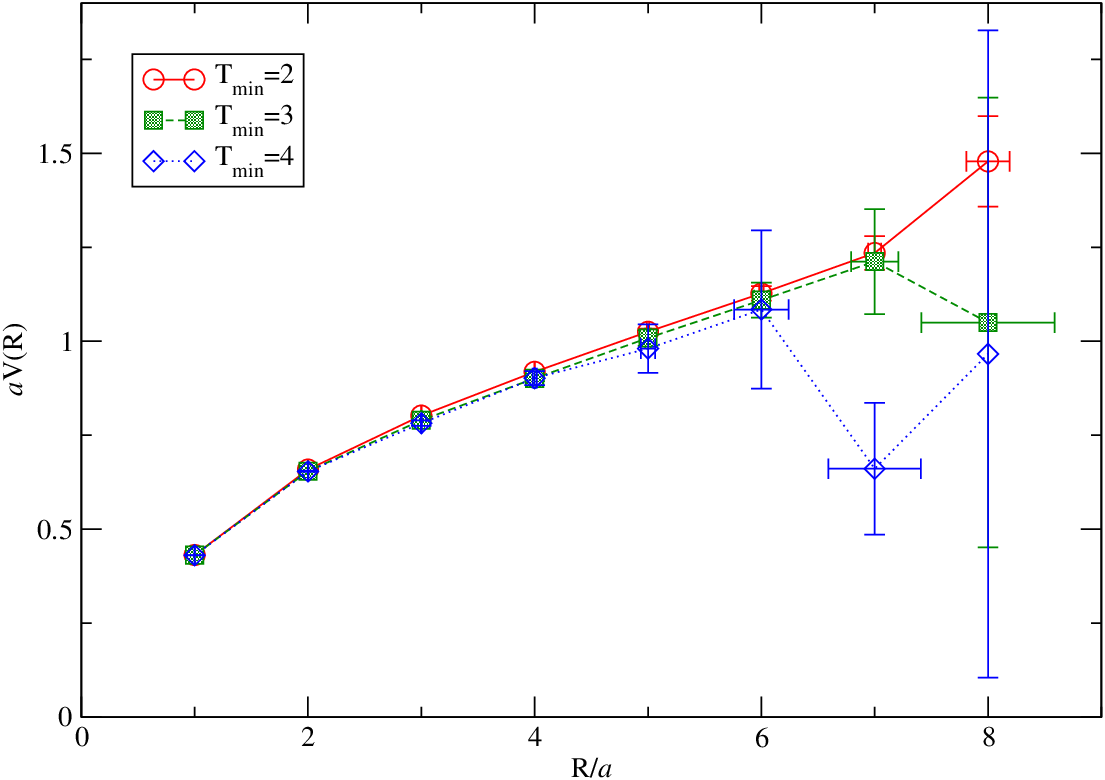
To determine the lattice spacing, we extracted the static quark potential from rectangular Wilson loops by fitting for . The lattice spacing was then determined by fitting the static quark potential to the Cornell form
| (3) |
and taking the string tension to be MeV. The static quark potential for the fine ensemble is shown in Fig. 1 and the best fit values are given in Table 2.
| (fm) | |||||
|---|---|---|---|---|---|
| 2 | 2.45 | ||||
| 3 | 1.25 | ||||
| 4 | 0.249 |
| Ensemble | (MeV) | (MeV) | |||
|---|---|---|---|---|---|
| Fine | 16 | 32 | 45 | 0.1–0.8 | 143–1142 |
| 16 | 20 | 71 | 0.1–0.7 | 143–999 | |
| 16 | 16 | 89 | 0.1–0.6 | 143–857 | |
| 16 | 12 | 119 | 0.1–0.6 | 143-857 | |
| Coarse | 12 | 24 | 47 | 0.25–1.1 | 277–1217 |
| 16 | 12 | 94 | 0.4–0.9 | 443–996 | |
| 16 | 8 | 141 | 0.4–0.7 | 443–775 | |
| Light | 12 | 24 | 43 | 0.1–0.8 | 104–834 |
| 16 | 12 | 87 | 0.1–0.8 | 104–834 | |
| 16 | 8 | 130 | 0.1–0.7 | 104–730 |
We have performed scans in at fixed temperature for four temperatures on the fine ensemble, and three temperatures on the light ensemble. The lattice volumes, temperatures and range of chemical potentials are given in table 3, along with those from the coarse ensemble that are used for comparison. For most of these temperatures and chemical potentials we have produced configurations at two values for the diquark source, namely on the fine ensemble, and on the light ensemble. A third diquark source value ( for the fine ensemble, for the light ensemble) has been added for selected parameter values to control the systematics of the extrapolations. For a few parameters, mostly at the highest and lowest -values, only a single -value has been used; in these cases, only results for the Polyakov loop, which is only weakly dependent on , will be shown here. In addition, we have performed temperature scans at fixed values of on the fine ensemble, with –4 corresponding to 63–356 MeV.
We note that by assigning a temperature to our ensembles with we deviate from what is commonly done in lattice thermodynamics studies. This is appropriate in the presence of a chemical potential (which modifies the temporal boundary conditions). At weak coupling and low temperature, relativistic quarks form a Fermi surface with Fermi momentum . The resulting ground state is highly degenerate, so that unlike the case when the discrete momenta on the finite volume do not lead to a large energy gap. For this reason in our view one should always consider as non-zero when studying systems with , even if .
For enhanced separation of scales , the behaviour as increases at zero temperature may be analysed using PT Kogut:2000ek, in this context an effective theory of tightly-bound mesons and baryons. For chiral symmetry of continuum QC2D is spontaneously broken from SU() to Sp() yielding Goldstones; for these are the pseudoscalar pion triplet and a scalar diquark/antidiquark pair. As is raised there is a second-order onset transition at to a phase where the baryon density and superfluid diquark condensate are both non-zero:
| (4) | ||||
| (5) |
Here is the chiral condensate at and the PT parameter known as the pion decay constant. Note that the onset transition in physical QCD is first order.
III Results from fine ensemble
III.1 Diquark condensation

Figure 2 shows the diquark condensate,
| (6) |
divided by the square of the chemical potential, as a function of chemical potential, for all temperatures. Physically, is the density of relativistic quark pairs contributing to the superfluid condensate. In the case of a weakly-coupled BCS condensate at the Fermi surface, this should be roughly equal to the momentum-space volume of a shell centred on the Fermi surface with thickness , the superfluid gap; by contrast leading order PT (4) predicts to be -independent for and hence the quantity plotted should fall off like .
For the two lowest temperatures, we find that is almost independent of both and for . This agrees with what was found previously for the coarse ensemble Cotter:2012mb. For the diquark condensate rises gradually from zero; we take this to be primarily an artefact of the linear extrapolation in .

To further investigate the diquark source dependence, in fig. 3 we show as function of for different values of the chemical potential. With our current data, we see no evidence of deviation from a linear form at any . Specifically, the form , which should hold exactly at , does not fit the data for any of our -values, even with the addition of a constant term. Fits to a more general power-law form, , yield powers ranging from for to at . The apparent linear -dependence at all may be an indication that non-analytic behaviour only sets in at lower -values than we have here. To improve on the diquark source extrapolation, it may be necessary to carry out a reweighting procedure as outlined in Brandt:2017oyy, or explore much smaller values of the source Braguta:2016cpw.
At MeV () we see that is significantly smaller for all values of , suggesting that this temperature is near the critical temperature for the superfluid to normal phase transition. This is again in agreement with what was found for the coarse lattice in Cotter:2012mb; Boz:2013rca. Finally, at the highest temperature, MeV (), the diquark condensate is consistent with zero, suggesting that at this temperature we are in the normal phase.

To study the superfluid to normal phase transition in more detail, we have performed temperature scans at fixed values of chemical potential and . These are fixed-scale temperature scans; i.e., the temperature is varied by changing , without changing the lattice spacing. This means that although our data for are not renormalised, this will just contribute an overall factor without changing the shape of the curves.
The results of these scans are shown in fig. 4. From the data extrapolated to using a linear Ansatz, we see evidence of a phase transition at MeV, independent of the chemical potential. In order to determine this transition in a more controlled manner, we find the inflection points for and 0.02 using a cubic spline interpolation, and extrapolate these to . The results are shown in table 4. This yields a somewhat lower temperature 90–100 MeV, which is consistent with the result quoted in Boz:2013rca, MeV. We note that the data are for a single volume and we can therefore not determine the order of the transition, but it is expected to be a second order transition (in the O(2) universality class), and the data are consistent with this.
| 0.3 | 0.4 | 0.5 | |
|---|---|---|---|
| 0.0782 | 0.0711 | 0.0715 | |
| 0.0734 | 0.0722 | 0.0677 | |
| 0.063(6)(3) | 0.075(8)(10) | 0.060(8)(6) | |
| (MeV) | 90(10) | 107(18) | 86(10) |
III.2 Deconfinement


Figure 5 shows the order parameter for deconfinement, the Polyakov loop , for our four different temperatures. The renormalised Polyakov loop is given in terms of the bare Polyakov loop and the temperature by
| (7) |
Just as in Boz:2013rca, we use two different renormalisation schemes,
| Scheme A | |||||
| Scheme B |
The results in fig. 5 have been obtained using Scheme A. We see no evidence of any deconfinement transition at our lowest temperature, MeV, corresponding to . This suggests that the high-density deconfinement transition found on coarser lattices at temperatures of 40–50 MeV Hands:2006ve; Cotter:2012mb is primarily a lattice artefact.
At higher temperatures we see that increases rapidly from zero above a chemical potential which is a decreasing function of temperature, in agreement with previous results.
To determine the transition line, we study the variation of the renormalised Polyakov loop with temperature at fixed values of the chemical potential . The results from Scheme B are shown in fig. 6. The results are indicative of a broadening of the transition and a reduction in the transition temperature as the chemical potential is increased. However, this effect is not large: the inflection point in Scheme B actually appears to increase between and , and even at our highest chemical potential, , the inflection point in Scheme B is still consistent with the inflection point in Scheme A. As can be seen from fig. 7, the transition in Scheme A happens at a considerably lower temperature than in Scheme B, which may be taken as an indication of the width of the crossover and associated uncertainty in the transition temperature. It would be useful to compare these scheme-dependent results with other quantities sensitive to deconfinement, such as the static quark potential Astrakhantsev:2018uzd or the entropy of a static quark Weber:2016fgn.
| 0.0 | 0.2 | 0.3 | 0.4 | 0.5 | |
|---|---|---|---|---|---|
| 0.1187 | 0.072–0.125 | 0.057–0.113 | 0.055–0.094 | ||
| — | 0.06–0.16 | 0.050–0.094 | 0.063–0.087 | ||
| 0.1362 | 0.10(5) | 0.073(30) | 0.075(20) | ||
| (MeV) | 194(4) | 143(70) | 105(45) | 107(30) | |
| 0.1813 | 0.1613 | 0.1561 | 0.1385 | ||
| — | 0.1565 | 0.1529 | 0.1423 | ||
| 0.164 | 0.147(3) | 0.147(12) | 0.150(6) | ||
| (MeV) | 234(10) | 210(4) | 210(17) | 214(9) |

Our results for the deconfinement transition temperature are shown in Table 5 and Fig. 8. We find a large discrepancy between the two schemes, and this discrepancy increases with ; however, the uncertainties are large, in particular in scheme A which has a lower . There are indications that, rather than decreasing monotonically towards 0 at large , approaches a constant value which is above (scheme B) or close to (scheme A) the superfluid transition temperature MeV. If this is confirmed, it means there is no deconfining transition at , and that the superfluid phase remains confined at all .

III.3 Quark number density
The final quantity to consider is the quark number density , which forms the basis for computing bulk thermodynamic properties such as the pressure. In figure 9 we show the quark number density extrapolated to zero diquark source (using a linear extrapolation) at the lowest temperature studied, corresponding to . As was the case for the diquark condensate, we do not find significant evidence of a deviation from a linear behaviour for the range of -values we have. The data are plotted in dimensionless form by normalising by the density for a gas of massless noninteracting fermions. Fig. 9 shows results obtained using two choices for : firstly using the continuum result
| (8) |
and secondly, using a form evaluated as a mode sum using the action (1,2) with and on a finite lattice as described in Hands:2006ve. Both forms were explored in Cotter:2012mb, with the conclusion that while offers a better correction for UV artifacts at large , it is prone to significant IR artifacts for , so that is preferred in this regime. In the current work we have addressed this issue by evaluating on a much larger spatial volume than that used for simulation, specifically (with checked to see that this was sufficient). This removes the IR artifacts but retains the UV corrections.
We find that rises rapidly above the onset transition, then descends to reach a plateau for MeV. This is in qualitative agreement with the predictions of PT shown in Fig. 3 of Hands:2006ve. Within the fairly large errors resulting from the extrapolation the results obtained in the neighbourhood of onset with continuum and lattice free fermions are compatible, but for MeV the curve continues to rise while the lattice normalisation yields a plateau with ; for the reasons given in the previous paragraph this is the normalisation we prefer and will use henceforth. Also shown in Fig. 9 is the ratio evaluated using free massive Wilson fermions with ; in this case the value of on the plateau is consistent with unity. Due to the difficulties inherent in assigning a bare quark mass for interacting Wilson fermions, we therefore do not draw any physical conclusions from the plateau height at this stage.
An important observation is that there is no longer evidence for a regime at high where increases above its value on the plateau (Cf. Fig. 11 of Cotter:2012mb; were the high- behaviour in that plot physical, then a corresponding rise would be expected on the fine lattice at MeV). In conclusion, at the lowest temperature studied the equation of state looks “quarkyonic”, ie. with , all the way along the -axis, with no evidence of a qualitative change associated with deconfinement. This is consistent with our results for the Polyakov loop, which show no sign of a deconfinement transition at low temperature, and the high- increase seen in Cotter:2012mb is therefore most likely a lattice artefact.

As shown in Fig. 10, this behaviour persists for the lowest three temperatures, which according to the results in section III.1 are all in the superfluid region (or near the transition temperature, for ). The data suggest the plateau value of falls with increasing , although uncertainties following the extrapolation are significant. At the highest temperature, MeV (), which falls in the quark–gluon plasma phase, we see indications of monotonically increasing with , in qualitative agreement with the findings of Cotter:2012mb.


To make this comparison quantitative, we show the results from the fine and coarse ensemble together, in units of the onset chemical potential (allowing also for a comparison of results for the different quark masses), in figure 11. At low temperature (upper panel) there is quantitative agreement between the two ensembles for . For larger the rise in seen for the coarse ensemble (which might have signalled a transition to a different state of matter) is absent for the fine ensemble, and instead we see that remains close to throughout. This is consistent with our results for the Polyakov loop, which show no sign of a deconfinement transition at low temperature, and the high- increase seen in Cotter:2012mb is therefore most likely a lattice artefact. The same pattern is repeated at high temperature (lower panel), where now we see approach from below. However, part of the difference between the two ensembles may in this case be due to the slightly different temperatures (120 vs 130 MeV for the fine and coarse ensembles respectively).

Next we discuss the pressure, which as outlined in Hands:2006ve; Cotter:2012mb can be obtained in the limit of low via an integral of the form . In order to arrive at the dimensionless ratio starting from our data there are several different quadrature schemes available: here we use
| (9) |
introduced as “scheme II” in Cotter:2012mb ( is the lowest available value in the dataset) . Reassuringly, with now defined on a large spatial volume to eliminate IR artifacts we find results compatible with those computed using scheme I, which was not the case in Cotter:2012mb. The results for data extrapolated to , at low temperatures where there are enough -points to control the numerical integration, are shown in Fig. 12.
The main result is that increases sharply after onset, reaching a plateau at . It appears to approach the plateau from below, in contrast to the PT prediction that the SB limit is approached from above Hands:2006ve. While, as in the discussion of , it is premature to assign a precise value to the height of the plateau, it is worth recalling that e.g. in the Van der Waals equation of state the ideal gas pressure receives a downward correction due to attractive forces between particles.
IV Results from light ensemble

We now study the effect that reducing the quark mass may have on the phase structure and equation of state. While our parameters are still very far from the chiral limit, this may give us an idea of which, if any, qualitative changes may occur as we approach this limit.
Figure 13 shows the diquark condensate from the light ensemble for our three different temperatures, extrapolated to . On the face of it, these results are qualitatively different from our results with heavier quarks, in that the diquark condensate no longer scales like in the region just above the onset transition. This might be taken as an indication that a BEC window is opening up where, rather than following the BCS scaling , the condensate behaves according to the predictions (4) of zero-temperature chiral perturbation theory.
To facilitate this comparison, we have included in fig. 13 the PT curve (4), with an arbitrary prefactor, and we see that the data for MeV make contact with this curve.
This interpretation is, however, complicated by our lack of control of the extrapolation. For nearly all points, we only have two values of the diquark source () available and have used a simple linear extrapolation. For and 0.3 on the lattice we also have data for , and have also used a quadratic extrapolation as well as a power law + constant form, . While the quadratic extrapolation gives results roughly consistent with the linear form, the power law form gives a result which is consistent with BCS scaling at all . It should be noted that near the onset transition, we expect a power-law scaling with .

We also find that also for , and we take this to be an indication that the linear extrapolation breaks down in this regime. Figure 14 shows the diquark condensate as a function of for those chemical potentials where we have 3 -values at our disposal. We see that the data are consistent with a linear behaviour as was also found for the fine ensemble, but may also be described with a power-law + constant form. A better control over the diquark source extrapolation, for example along the lines of Brandt:2017oyy, is required to determine whether there is indeed a BEC window for these parameters.
The results for are almost identical to those for MeV, except for MeV. However, at the highest temperature, MeV () we see that the diquark condensate is much smaller, and vanishes at high . It is worth noting, however, that does not vanish at all , as was the case at comparable temperatures for the coarse and fine ensembles. This may be taken as a first indication of a -dependent superfluid to normal transition temperature. A controlled extrapolation combined with temperature scans at fixed would be required to draw a firm conclusion.

Looking now at the deconfinement transition, figure 15 shows the Polyakov loop as function of chemical potential for our three temperatures. In the absence of a temperature scan to fix the renormalisation constant, we show the unrenormalised Polyakov loop. This does not affect the shape of each of the curves, only the relative magnitude of the data at different temperatures. We see the same picture as before, where at low temperature (except for MeV, corresponding to , which in the light of previous results we attribute to a lattice artefact), but increasing with at higher temperature. At MeV (), we note that also at , suggesting that this temperature is near the transition region for this ensemble.


In fig. 16 we show the quark number density calculated using the same procedure outlined in Sec. III.3. At low temperature, this has a plateau for , in line with our previous results, while at high temperature we see a steeper increase with , as seen before, which is much more pronounced than that for the fine lattice shown in Fig. 10. On a coarse lattice the impact of UV artefacts in this regime cannot be excluded. However, as can be seen in the lower panel of fig. 16, the quark number density at the lowest temperature is also consistent with the PT prediction (5), as indicated by the extrapolated curve tending to a non-zero constant as . It therefore remains an open question whether we for these parameters have a window characterised by a Bose–Einstein condensate of tightly bound diquarks.
In figure 11 we compare our results for the quark number density with those obtained on the coarse ensemble in Cotter:2012mb. We see that the smaller quark mass has a large quantitative effect, giving a much lower number density. Because is now smaller, the increase in at large , which is likely to be a lattice artefact, now only appears at larger . At high temperature, however, we do not see any plateau in , as was the case for the fine ensemble, but instead a monotonic increase with .
Finally, we note that results for for the light ensemble are included in Fig. 12. The notable feature is that the rise from zero following onset is now much steeper, and an approximate plateau established by . As before, we are reluctant to over-interpret the disparity in plateau height between fine and light ensembles.
V Conclusions and outlook
We have performed lattice simulations of two-colour QCD at different lattice spacings and different quark masses, as a step towards the continuum and chiral (or light-quark) limits of this theory. Our investigation of the phase structure of the theory in the plane has yielded results in qualitative agreement with earlier studies Hands:2010gd; Cotter:2012mb; Boz:2013rca; most notably it has confirmed the quarkyonic phase at low and intermediate to high . In this phase, quarks are confined but the bulk thermodynamics as well as the diquark condensate behave as if the system consists of a Fermi sphere of weakly interacting quarks. This phase is found to extend to larger as the lattice spacing or the quark mass is reduced. A striking result is that at the lowest temperatures explored the quark number density is found to be very close to the Stefan–Boltzmann value. Because we have not yet determined the physical quark mass, it is not possible to state with confidence whether the ratio is greater or less than one in this regime. However, Fig. 16 does suggest that the ratio falls as the quark mass decreases.
The superfluid phase transition temperature is found to be independent of at least for our heavier quark mass, corresponding to . The transition temperature MeV is in quantitative agreement with that found on a coarser lattice in Boz:2013rca. This qualitative behaviour also agrees with what has been found for QCD at high isospin density Brandt:2017oyy. For lighter quarks, however, there are indications that may increase with .
Although we find a deconfinement transition at high temperature, the deconfinement transition previously seen at low and high appears to be a lattice artefact — at MeV the Polyakov loop appears to increase from zero at for all lattice parameters. Simulations using staggered fermions at a relatively high temperature MeV Braguta:2016cpw; Astrakhantsev:2018uzd have found a deconfinement transition at MeV characterised by the string tension dropping to zero. This is not in contradiction with the absence of any deconfinement transition at MeV.
The location of the high-temperature deconfinement transition is not yet clear. Our results suggest a broad crossover with a transition temperature that decreases with increasing . The analysis is complicated by lack of precise data for the renormalised Polyakov loop at low temperature, as well as a small but nontrivial diquark source dependence. There are indications that may tend to a constant at large and that for all .
There remain significant uncertainties relating to the extrapolation to zero diquark source , with our data unable to distinguish between a linear -dependence and the nonanalytic behaviour expected at least in the vicinity of the onset transition. This may be mitigated by adopting the reweighting method introduced in Brandt:2017oyy and implemented in the context of QC2D in Iida:2019rah; this will be left for future investigations.
Another source of uncertainty is the use of relatively small volumes, with for our lowest temperatures. Additional simulations on larger volumes would be required to reliably determine if our assignment of a nonzero temperature to these ensembles is correct. We note that finite volume effects were studied previously in Ref. Cotter:2012mb; there it was found that the results for the various physical quantities, and in particular the Polyakov loop, agreed between the two volumes considered, suggesting that finite volume effects are indeed small.
A reliable continuum extrapolation would require significantly finer lattices than those used in this study. The first step towards further reducing the lattice spacing errors would be to employ an improved fermion action. This, together with algorithmic improvements, would also allow us to study lighter quark masses which are out of bounds with the unimproved Wilson action used here.
Acknowledgements.
This work used the DiRAC Blue Gene Q Shared Petaflop system at the University of Edinburgh, operated by the Edinburgh Parallel Computing Centre on behalf of the STFC DiRAC HPC Facility (www.dirac.ac.uk). This equipment was funded by BIS National E-infrastructure capital grant ST/K000411/1, STFC capital grant ST/H008845/1, and STFC DiRAC Operations grants ST/K005804/1 and ST/K005790/1. DiRAC is part of the National E-Infrastructure. JIS and TSB acknowledge the support of Science Foundation Ireland grants 11-RFP.1-PHY3193 and 11-RFP.1-PHY3193-STTF-1. SJH was supported by STFC grant ST/L000369/1. We acknowledge the support of COST Action CA15213 “Theory of relativistic heavy-ion collisions”. PG thanks the Institute for Theoretical Physics of the University of Münster where part of the work was done. JIS expresses his deep appreciation for the hospitality of the Galileo Galilei Institute, Florence, where this work was completed.References
- (1) K. Langfeld, Density-of-states, PoS LATTICE2016, 010 (2017), [arXiv:1610.09856].
- (2) E. Seiler, Status of complex Langevin, EPJ Web Conf. 175, 01019 (2018), [arXiv:1708.08254].
- (3) L. Scorzato, The Lefschetz thimble and the sign problem, PoS LATTICE2015, 016 (2016), [arXiv:1512.08039].
- (4) A. Alexandru, G. Basar, P. F. Bedaque, G. W. Ridgway and N. C. Warrington, Sign problem and Monte Carlo calculations beyond Lefschetz thimbles, JHEP 05, 053 (2016), [arXiv:1512.08764].
- (5) B. B. Brandt, G. Endrődi and S. Schmalzbauer, QCD phase diagram for nonzero isospin-asymmetry, Phys. Rev. D97, 054514 (2018), [arXiv:1712.08190].
- (6) S. Hands, S. Kim and J.-I. Skullerud, A quarkyonic phase in dense two color matter?, Phys. Rev. D81, 091502R (2010), [arXiv:1001.1682].
- (7) S. Cotter, P. Giudice, S. Hands and J.-I. Skullerud, Towards the phase diagram of dense two-color matter, Phys.Rev. D87, 034507 (2013), [arXiv:1210.4496].
- (8) T. Boz, S. Cotter, L. Fister, D. Mehta and J.-I. Skullerud, Phase transitions and gluodynamics in 2-colour matter at high density, Eur.Phys.J. A49, 87 (2013), [arXiv:1303.3223].
- (9) A. Maas, L. von Smekal, B. Wellegehausen and A. Wipf, The phase diagram of a gauge theory with fermionic baryons, Phys.Rev. D86, 111901 (2012), [arXiv:1203.5653].
- (10) B. H. Wellegehausen, A. Maas, A. Wipf and L. von Smekal, Hadron masses and baryonic scales in -QCD at finite density, Phys. Rev. D89, 056007 (2014), [arXiv:1312.5579].
- (11) L. He, Nambu–Jona-Lasinio model description of weakly interacting Bose condensate and BEC–BCS crossover in dense QCD-like theories, Phys. Rev. D82, 096003 (2010), [arXiv:1007.1920].
- (12) J. O. Andersen, T. Brauner and W. Naylor, Confronting effective models for deconfinement in dense quark matter with lattice data, Phys. Rev. D92, 114504 (2015), [arXiv:1505.05925].
- (13) T. Kojo and G. Baym, Color screening in cold quark matter, Phys. Rev. D89, 125008 (2014), [arXiv:1404.1346].
- (14) D. Suenaga and T. Kojo, Gluon propagator in two-color dense QCD: Massive Yang-Mills approach at one-loop, Phys. Rev. D100, 076017 (2019), [arXiv:1905.08751].
- (15) N. Strodthoff and L. von Smekal, Polyakov-quark-meson-diquark model for two-color QCD, Phys. Lett. B731, 350 (2014), [arXiv:1306.2897].
- (16) N. Khan, J. M. Pawlowski, F. Rennecke and M. M. Scherer, The phase diagram of QC2D from functional methods, arXiv:1512.03673.
- (17) R. Contant and M. Q. Huber, Phase structure and propagators at nonvanishing temperature for QCD and QCD-like theories, Phys. Rev. D96, 074002 (2017), [arXiv:1706.00943].
- (18) R. Contant and M. Q. Huber, Dense two-color QCD from Dyson–Schwinger equations, Phys. Rev. D101, 014016 (2020), [arXiv:1909.12796].
- (19) S. Hands, S. Kim and J.-I. Skullerud, Deconfinement in dense 2-color QCD, Eur. Phys. J. C48, 193 (2006), [hep-lat/0604004].
- (20) J. Kogut, M. Stephanov, D. Toublan, J. Verbaarschot and A. Zhitnitsky, QCD-like theories at finite baryon density, Nucl. Phys. B582, 477 (2000), [hep-ph/0001171].
- (21) V. V. Braguta, E. M. Ilgenfritz, A. Yu. Kotov, A. V. Molochkov and A. A. Nikolaev, Study of the phase diagram of dense two-color QCD within lattice simulation, Phys. Rev. D94, 114510 (2016), [arXiv:1605.04090].
- (22) N. Yu. Astrakhantsev et al., Lattice study of static quark-antiquark interactions in dense quark matter, JHEP 05, 171 (2019), [arXiv:1808.06466].
- (23) J. Wilhelm, L. Holicki, D. Smith, B. Wellegehausen and L. von Smekal, Continuum Goldstone spectrum of two-color QCD at finite density with staggered quarks, Phys. Rev. D100, 114507 (2019), [arXiv:1910.04495].
- (24) K. Iida, E. Itou and T.-G. Lee, Two-colour QCD phases and the topology at low temperature and high density, JHEP 01, 181 (2020), [arXiv:1910.07872].
- (25) TUMQCD, J. H. Weber, Single quark entropy and the Polyakov loop, Mod. Phys. Lett. A31, 1630040 (2016), [arXiv:1606.06193].