跳到论文正文
W Papers独立论文阅读器 arXiv:1912.10862 论文正文 计算阅读时间 · 0%
引用这篇论文根据当前论文元数据生成,正式投稿前建议核对。


License: arXiv.org perpetual non-exclusive license
arXiv:1912.10862v2 [math.AP] 31 Dec 2019

From point vortices to vortex patches in self-similar expanding configurations

Samuel Zbarsky    Princeton University
Abstract

The main result is that given a generic self-similarly expanding configuration of 3 point vortices that start sufficiently far out, we can instead take compactly supported vorticity functions, and the resulting solution to 2D incompressible Euler will evolve like a nearby point vortex configuration for all time, with the size of the patches growing at most as t1/4+ϵt^{1/4+\epsilon} and the distance between them growing as t\sqrt{t}.

1 Introduction

We study the 2D Euler equation for u:ℝ2→ℝ2u:\mathbb{R}^{2}\to\mathbb{R}^{2}

∂tu+u⋅∇u+∇p=0,∇⋅u=0\partial_{t}u+u\cdot\nabla u+\nabla p=0,\nabla\cdot u=0

The equation can be rewritten in terms of the vorticity

ω=∂1u2−∂2u1\omega=\partial_{1}u_{2}-\partial_{2}u_{1}

as follows:

∂tω⁡(x)\displaystyle\partial_{t}\omega(x) =u​(x)⋅∇ω​(x)\displaystyle=u(x)\cdot\nabla\omega(x)
u\displaystyle u =K∗ω\displaystyle=K*\omega

where, by rescaling time to avoid factors of 2​π2\pi, we can take

K⁡(x)=x⟂/|x|2.K(x)=x^{\perp}/|x|^{2}.

Thus the vorticity is transported by uu, which is generated as a singular integral of the vorticity. In this paper, we construct solutions that consist of three vortex patches (not necessarily smooth), each growing slowly in time, with the distance between the patches growing as t\sqrt{t}. We will obtain that the trajectories of the centers of mass of these patches behave approximately like point vortices, so we will first discuss what is known about point vortex systems. A point vortex system consists of nn point vortices, with masses Ωi\Omega_{i} and positions xix_{i}, whose motion is described by the ODE system

dd​t​xi=∑j≠iΩj​(xi−xj)⟂|xi−xj|2.\frac{d}{dt}x_{i}=\sum_{j\neq i}\Omega_{j}\frac{(x_{i}-x_{j})^{\perp}}{|x_{i}-x_{j}|^{2}}.

Here, as with the vorticity formulation of 2D Euler, we rescaled time to avoid factors of 2​π2\pi. This ODE is meant to model a fluid in which vorticity is highly concentrated around a few points. Some information about the behavior of solutions to this ODE can be found in [1]. While there are specific solutions in which vortices collide, for generic initial data, this does not happen [7, 24]. Rigorous justification of the point vortex model is provided in [23]. They show that if one replaces point vortices by signed L∞L^{\infty} localized vorticity, the solution to Euler will approximate the solution to the ODE over a fixed time interval. The assumptions on the L∞L^{\infty} bound of the solution are then significantly weakened in independent and simultaneous works by Marchioro in [22] and by Serfati in [27], with [27] giving better approximation of point vortices. One can view these as being almost L1L^{1} results. Both the assumptions on the L∞L^{\infty} bound on vorticity and the conclusion are further improved by Serfati in [28].

There are several observations about the long-term behavior of solutions to point vortex systems. First, if all masses are positive, then the solution will remain bounded. Second, it is easy to obtain solutions where two point vortices with masses Ω\Omega and −Ω-\Omega go off to infinity with their velocity approaching some nonzero limit. Third, there are point vortex systems that expand and spiral in a self-similar way so that the distance between the point vortices grows as t\sqrt{t}. An analysis of such self-similarly evolving 3-vortex system can be found in [1]. Some self-similarly evolving 4 and 5 vortex systems are constructed and analyzed in [25]. Some numerics for self-similarly evolving systems with more vortices may be found in [18].

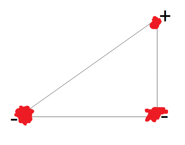
The centers of mass of the patches we construct will behave approximately like a self-similarly expanding 3-vortex system, see Figure 1 (for the precise statement, see Theorem 2 below).

Refer to caption
Refer to caption
Figure 1: An example of a self-similarly expanding 3-vortex system and a corresponding solution involving three vortex patches

In fact, part of the result may be viewed as an orbital stability statement for the centers of mass of the three patches relative a self-similarly expanding system. The radius of each of the three patches will grow at most like t1/4+ϵt^{1/4+\epsilon}. We will get this behavior for any three initial vortex patches, provided they have the right signs, are initially supported inside specified open balls, and have the correct total vorticity. In particular, this is the first construction where the support of the vorticity is known to go off to infinity that does not rely on symmetry. One consequence of not relying on symmetry is that this proof may generalize to exterior domains, where the shape of the domain itself may have no symmetries.

Before understanding the behavior of the three vortex patches, we first need to understand a single vortex patch, so we will now discuss the previously known results regarding vortex patches. Yudovich [29] showed global well-posedness for solutions with ω∈L1∩L∞\omega\in L^{1}\cap L^{\infty}. Given global well-posedness, it is natural to study the long-term behavior of vorticity. It was shown by Kirchhoff that elliptical patches will rotate uniformly [17]. Other rotating solutions with mm-fold symmetry bifurcating from the disk, called V-states, were found numerically by Deem–Zabusky [6] and proved to exist by Burbea [3]. For other results about rotating solutions, see [9] and results they cite. Aside from such special solutions, it is known that if the vorticity is the indicator function of a set with Ck,γC^{k,\gamma} boundary, then this regularity of the boundary will continue for all time, as shown by Chemin [4], Bertozzi–Constantin [2], and Serfati [26]. For other results concerning regularity and long-term behavior of vortex patches, see [8] and results they cite.

However, very little is known if no additional regularity is assumed. In particular, one can ask what happens if vorticity is initially compactly supported and L∞L^{\infty}. We will go over some results bounding the expansion of the support, known as vorticity confinement results. It is easy to see that the radius of the support can grow at most linearly, since uu is bounded. If vorticity is of a definite sign, then the radius of the support grows more slowly. In fact, it is not known whether it ever goes to infinity. Marchioro [20] showed an upper bound of t1/3t^{1/3} by using conservation of the second moment of vorticity. This was independently improved to (t​log⁡t)1/4(t\log t)^{1/4} by Iftimie–Sideris–Gamblin [16] and to t1/4log∘⋯∘logtt^{1/4}\log\circ\cdots\circ\log t by Serfati [27], with the improvement coming largely from using conservation of the center of mass of the vorticity. Compare this with the present work, in which we get the slightly worse bound of t1/4+ϵt^{1/4+\epsilon} for each of the vortex patches. There are also several other vorticity confinement results, including getting similar confinement bounds, but depending on the L2+ϵL^{2+\epsilon} norm rather than the L∞L^{\infty} norm of vorticity [19]. Compare this to the result in [27], which requires an L∞L^{\infty} bound, but the constant in the confinement bound has very weak dependence on the L∞L^{\infty} norm (it is linear in log∘⋯∘log||ω||L∞)\log\circ\cdots\circ\log||\omega||_{L^{\infty}}), depending mostly on the L1L^{1} norm. There are also various bounds on confinement of positive compactly supported vorticity in other domains. In particular, on the upper half-plane, the xx coordinate of the center of mass of vorticity is at least c​tct and the yy coordinate of points in the support is bounded by C​(t​log⁡t)1/3C(t\log t)^{1/3} [10], while the xx coordinate of points in the support is at least −C​(t​log⁡t)1/2-C(t\log t)^{1/2} [12]. The latter work also analyzes what possible weak limits a positive vorticity solution can have on a half-plane (under appropriate rescaling). In exterior domains, the radius of the support is bounded by C​t1/2Ct^{1/2}, with further improvements in the exponent when the domain is the exterior of a disk [21, 14]. On 𝕋×ℝ\mathbb{T}\times\mathbb{R}, the yy coordinate of points in the support is bounded by C​t1/3​log2​tCt^{1/3}\log^{2}t [5]. A survey of various related results can be found in [11]. However, things are very different if you allow mixed-sign vorticity. [16] contains a construction of a compactly supported positive vorticity vortex patch in the first quadrant of the plane, reflected into the other quadrants with changing sign, whose support grows linearly. However, the proof relies heavily on the symmetry, so it is very unstable and can only give this result for a system with total vorticity 0.

Returning to the plane, but now without a definite sign, there is a vorticity confinement result by Iftimie–Lopes Filho–Nussenzveig Lopes that addresses the question of weak limits under appropriate rescaling [13]. This result states that if we define

ω~α​(x,t)=t2​α​ω​(tα​x,t)\tilde{\omega}_{\alpha}(x,t)=t^{2\alpha}\omega(t^{\alpha}x,t)

for α>1/2\alpha>1/2, then

ω~α⇀t→∞m​δ0\tilde{\omega}_{\alpha}\xrightharpoonup[t\to\infty]{}m\delta_{0}

in the weak-* sense for measures where m=∫ω​𝑑xm=\int\omega dx and δ0\delta_{0} is the Dirac delta. The authors interpret this as showing confinement of net vorticity to a radius of t\sqrt{t}, but this result still allows for strange examples like having both positive and negative vortex patches moving away from the origin in different directions and being at distance t2/3​log⁡tt^{2/3}\log t. Our result shows that we cannot take α=1/2\alpha=1/2 in the statement of [13] and thus, in a sense, net vorticity is moving off to infinity. In fact, the solution given here should, modulo a rotation by a logarithmically growing angle, weakly converge to a sum of three delta masses under the rescaling with α=1/2\alpha=1/2.

The last previous result we discuss is a paper by Iftimie–Marchioro [15], which looked at a toy model of the construction given here and showed confinement of the vortex patches. The toy model consists of taking a self-similarly expanding point vortex system, replacing only one of the point vortices with a patch, assuming that the trajectory of the other point vortices is fixed, and seeing how the patch evolves. The purpose of looking at the toy model was to sidestep the issue of stability for self-similar point vortex systems. and only worry about confinement of vorticity. For some configurations, they bound the radius of the support of the patch as growing no faster than t(1+α)/3t^{(1+\alpha)/3} for α\alpha some constant that depends on the configuration, is always positive, and is less than 1/2. This means that the vortex patch size grows slower than the distance between patches. In this paper, we solve the full problem for self-similar expanding three-vortex systems, replacing each of the three vortices with vortex patches, allowing a generic self-similarly expanding configuration of 3 vortices, and obtaining that the radius of support grows at most as t1/4+ϵt^{1/4+\epsilon} for any given ϵ>0\epsilon>0. The improvement in the exponent from 1/31/3 to 1/41/4 comes from actually analyzing the stability and keeping track of the center of mass, in the same way that using conservation of center of mass gives the same improvement for a single vortex patch. To get rid of α\alpha, we obtain a better bound on moment growth by noticing that one of the expressions that shows up in the expression for moment derivatives is the approximate derivative of another expression and thus obtaining some cancellation in the most troublesome term (one can also think of this as a renormalization of the moments). Our result is limited to 3 vortex system due to the stability analysis, and if one found stably growing systems of 4 or more vortices, the confinement result would most likely carry over with little modification. However, one needs sufficiently good stability results; orbital linear stability, which may not be hard to obtain for some systems, is not enough. Our assumptions on the patches, same as in [15], will be that the vorticity ω\omega is compactly supported and L2+ϵL^{2+\epsilon} (note that a smaller ϵ\epsilon both expands this class and improves vortex patch confinement, so this is not a tradeoff). Technically, we need to assume that ω∈L∞\omega\in L^{\infty} to make use of the well-posedness theory, but all constants in the proof will only depend on the L2+ϵL^{2+\epsilon} bound. We need this bound in many places in the proofs in order to bound integrals of 1|x−a|​ω​(x)\frac{1}{|x-a|}\omega(x) using Holder’s inequality.

2 Point vortex systems

In order to state the main result, we first need to analyze some properties of expanding systems of three point vortices. Take any three vortex system. It has four conserved quantities, each of which is easy to check.

  1. 1.

    X=∑ixi​ΩiX=\sum_{i}x_{i}\Omega_{i} (this has two components)

  2. 2.

    I=∑iΩi​|xi|2I=\sum_{i}\Omega_{i}|x_{i}|^{2}

  3. 3.

    E=∑i≠jΩi​Ωj​log⁡|xi−xj|E=\sum_{i\neq j}\Omega_{i}\Omega_{j}\log|x_{i}-x_{j}|.

Now suppose we take a self-similarly expanding solution with three point vortices and nonzero total mass. By moving the origin, we can assume that X=0X=0. Then self-similarity ensures that I=C​tI=Ct for some constant CC.Then conservation of II and EE ensure that

Ω1​Ω2+Ω1​Ω3+Ω2​Ω3\displaystyle\Omega_{1}\Omega_{2}+\Omega_{1}\Omega_{3}+\Omega_{2}\Omega_{3} =0\displaystyle=0 (1)
I\displaystyle I =0\displaystyle=0 (2)

We move the rest of the analysis to the following lemma, proved in the appendix:

Lemma 1.

Suppose we have a point vortex system (yi,Ωi)(y_{i},\Omega_{i}) satisfying X=0X=0, (1), and (2). Suppose furthermore that y1,y2,y3y_{1},y_{2},y_{3} are not the vertices of an equilateral triangle and are not collinear and that they evolve as a self-similarly expanding system.

  1. 1.

    ∑Ωi≠0\sum\Omega_{i}\neq 0.

  2. 2.

    Take the subspace VV of vortex locations that satisfy X=0X=0. There exists a two-dimensional surface SS through (yi)(y_{i}) and coordinates on some neighborhood UU of (y1,y2,y3)(y_{1},y_{2},y_{3}) in AA such that two of the coordinates are the angle of rotation and the ratio of dilation needed to hit some z∈Sz\in S and the other two coordinates are I⁡(z)I(z) and E⁡(z)E(z) at the resulting point of SS.

Note that for the second part of the lemma statement, it is important that II is evaluated at the point z∈Sz\in S, not at the original point xx.

The conditions in the lemma statement are generic for self-similarly expanding 3-vortex configurations; one system satisfying the hypotheses of the lemma is the following example, taken (up to sign reversal) from [24]. Let Ω1=−2\Omega_{1}=-2, Ω2=−2\Omega_{2}=-2, Ω3=1\Omega_{3}=1 and x1=(−1,0)x_{1}=(-1,0), x2=(1,0)x_{2}=(1,0), x3=(1,2)x_{3}=(1,\sqrt{2}). Then translate to achieve X=0X=0. This example is shown in Figure 1.

3 Result statement and stability of centers of mass

We can now state the main result precisely.

Theorem 2.

Take an arrangement of three points (yi,Ωi)(y_{i},\Omega_{i}) satisfying the conditions of Lemma 1. Let ϵ>0\epsilon>0, be arbitrary and small, M>0M>0, ρ>0\rho>0 be arbitrary. Then there exists some T>0T>0 so that for t0>Tt_{0}>T, if we take the solution {(t0​yi,Ωi)}\{(\sqrt{t_{0}}y_{i},\Omega_{i})\} and replace each point vortex (xi,Ωi)(x_{i},\Omega_{i}) with an L∞L^{\infty} vorticity function ωi\omega_{i} such that:

  1. 1.

    The center of mass of the whole system is still 0.

  2. 2.

    supp⁡ωi⊆B⁡(xi,ρ)\supp\omega_{i}\subseteq B(x_{i},\rho).

  3. 3.

    ‖ωi‖L2+ϵ≤M||\omega_{i}||_{L^{2+\epsilon}}\leq M.

  4. 4.

    ωi\omega_{i} has definite sign.

  5. 5.

    ∫ωi=Ωi\int\omega_{i}=\Omega_{i}.

then at each later time tt, there exists some {(zi​(t))}∈S\{(z_{i}(t))\}\in S with |zi−yi|<ϵ|z_{i}-y_{i}|<\epsilon, some angle β⁡(t)\beta(t), and some factor 𝑂𝑃𝐸𝑁γ⁡(t)=(1+O⁡(ϵ))​t)\gamma(t)=(1+O(\epsilon))\sqrt{t}) such that, letting xi=Rβ​γ​zix_{i}=R_{\beta}\gamma z_{i}, the solution at time tt is ∑ωi\sum\omega_{i} with:

  1. 1.

    xi=1Ωi​∫ωi​(x)​x​𝑑xx_{i}=\frac{1}{\Omega_{i}}\int\omega_{i}(x)xdx.

  2. 2.

    supp⁡ωi⊆B⁡(xi,ϵ​t1/4+ϵ)\supp\omega_{i}\subseteq B(x_{i},\epsilon t^{1/4+\epsilon}).

  3. 3.

    ∫ωi=Ωi\int\omega_{i}=\Omega_{i}.

  4. 4.

    ωi\omega_{i} has definite sign.

There are a couple of comments about the statement. First, because of how we defined xix_{i} and SS, we have that β\beta and γ\gamma are uniquely defined by the arrangement. Second, condition 1 in the theorem statement is simply for convenience–since ∑Ωi≠0\sum\Omega_{i}\neq 0, we could restate the theorem without this condition, but adding a translation to move the center of mass to 0. Third, for the theorem as stated, for different ϵ\epsilon one needs different data. However, by being much more careful, and with some modification of the bootstrap assumptions, one can probably modify the proof to find some TT so that the radius of the support of each ωi\omega_{i} grows like t1/4+o⁡(1)t^{1/4+o(1)}. Finally, a version of this theorem and proof probably holds for exterior domains. One would need to use the fact that in exterior domains, when |x|,|y|∼t|x|,|y|\sim\sqrt{t}, we have K⁡(x,y)≈(x−y)⟂|x−y|2K(x,y)\approx\frac{(x-y)^{\perp}}{|x-y|^{2}} (using the more precise asymptotics found in [14]). The theorem statement would need to be modified slightly since center of mass is no longer conserved.

Proof.

kk will denote an even integer and δ\delta will denote some sufficiently small constant that can depend on kk and RR will denote some large constant that depends on δ\delta. At the end of the proof, we will choose kk, δ\delta, and RR depending on the initial configuration of point vortices, as well as ϵ,ρ,M\epsilon,\rho,M. We will then choose TT large enough depending on ϵ,ρ,M,k,δ\epsilon,\rho,M,k,\delta. All constants CC in the statement and proof (including implicit constants hidden by OO notation) can depend on the initial configuration of point vortices, as well as ϵ,ρ,M,k\epsilon,\rho,M,k, but not on RR or δ\delta. The letters CC may be used for different constants on different lines. We will use O^\hat{O} if we’re allowing the implicit constant to depend on the initial configuration of point vortices and on nothing else. At any time tt, let

xi​(t)\displaystyle x_{i}(t) =1Ω​∫x​ωi​(x)​𝑑x\displaystyle=\frac{1}{\Omega}\int x\omega_{i}(x)dx
Ik,i​(t)\displaystyle I_{k,i}(t) =∫|x−x~i|k​ωi​(x)​𝑑x\displaystyle=\int|x-\tilde{x}_{i}|^{k}\omega_{i}(x)dx

We will have the following bootstrap assumptions:

  1. 1.

    xi=Rβ​γ​zix_{i}=R_{\beta}\gamma z_{i} with |zi−yi|<ϵ2|z_{i}-y_{i}|<\epsilon^{2} for some angle β⁡(t)\beta(t), and some factor γ⁡(t)\gamma(t) satisfying |γt−1|<ϵ|\frac{\gamma}{\sqrt{t}}-1|<\epsilon

  2. 2.

    I2,i<tϵ/2I_{2,i}<t^{\epsilon/2}

  3. 3.

    Ik,i<tk⁡(1+ϵ)/4I_{k,i}<t^{k(1+\epsilon)/4}

  4. 4.

    ω1,ω2,ω3\omega_{1},\omega_{2},\omega_{3} are three L2+ϵL^{2+\epsilon} compactly supported functions of definite sign, ‖ωi‖L2+ϵ≤M\|\omega_{i}\|_{L^{2+\epsilon}}\leq M

  5. 5.

    supp⁡ωi⊆B⁡(xi,ϵ​t1/4+ϵ)\supp\omega_{i}\subseteq B(x_{i},\epsilon t^{1/4+\epsilon}), that is |p−xi|<ϵ​t1/4+ϵ|p-x_{i}|<\epsilon t^{1/4+\epsilon} for any p∈supp⁡ωip\in\supp\omega_{i}.

These assumptions hold at time t0t_{0} as long as TT is big enough. If they always hold, we are done, so we can assume that the first time when one of them fails is T∗<∞T_{*}<\infty.

First, we want to understand the ODE satisfied by the triple (x1,x2,x3)(x_{1},x_{2},x_{3}) of centers of mass of the patches in order to verify bootstrap assumption 1. First note that from the conservation of the center of mass of the vorticity, we get that ∑Ωi​xi=0\sum\Omega_{i}x_{i}=0, so the center of mass of ziz_{i} stays at 0. We will use the notation Ix=∑Ωi​|xi|2I_{x}=\sum\Omega_{i}|x_{i}|^{2} and Iz=∑Ωi​|zi|2I_{z}=\sum\Omega_{i}|z_{i}|^{2}. Because of condition 1, there is so need to make this distinction for EE. For this calculation, we note that from the bootstrap assumptions, for x∈supp⁡ωix\in\supp\omega_{i}, y∈supp⁡ωjy\in\supp\omega_{j} with j≠ij\neq i, we have

(x−y)⟂|x−y|2=(xi−xj)⟂|xi−xj|2+A1​(x−xi)+A2​(y−xj)+O⁡(|x−xi|2+|y−xj|2|xi−xj|3)\frac{(x-y)^{\perp}}{|x-y|^{2}}=\frac{(x_{i}-x_{j})^{\perp}}{|x_{i}-x_{j}|^{2}}+A_{1}(x-x_{i})+A_{2}(y-x_{j})+O\left(\frac{|x-x_{i}|^{2}+|y-x_{j}|^{2}}{|x_{i}-x_{j}|^{3}}\right)

where A1,A2A_{1},A_{2} are some linear functions dependent on tt. Then

dd​t​xi\displaystyle\frac{d}{dt}x_{i} =1Ωi​∬ωi​(x)​ωi​(y)​(x−y)⟂|x−y|2​𝑑x​𝑑y+∑j≠i∬ωi​(x)​ωj​(y)​(x−y)⟂|x−y|2​𝑑x​𝑑y\displaystyle=\frac{1}{\Omega_{i}}\iint\omega_{i}(x)\omega_{i}(y)\frac{(x-y)^{\perp}}{|x-y|^{2}}dxdy+\sum_{j\neq i}\iint\omega_{i}(x)\omega_{j}(y)\frac{(x-y)^{\perp}}{|x-y|^{2}}dxdy
=1Ωi[12∬ωi(x)ωi(y)((x−y)⟂|x−y|2+(y−x)⟂|y−x|2)dxdy\displaystyle=\frac{1}{\Omega_{i}}\Bigg[\frac{1}{2}\iint\omega_{i}(x)\omega_{i}(y)\left(\frac{(x-y)^{\perp}}{|x-y|^{2}}+\frac{(y-x)^{\perp}}{|y-x|^{2}}\right)dxdy
+∑j≠iΩi(x)Ωj(y)(xi−xj)⟂|xi−xj|2+O(∑j=13Ijt3/2)]\displaystyle\qquad+\sum_{j\neq i}\Omega_{i}(x)\Omega_{j}(y)\frac{(x_{i}-x_{j})^{\perp}}{|x_{i}-x_{j}|^{2}}+O\left(\sum_{j=1}^{3}\frac{I_{j}}{t^{3/2}}\right)\Bigg]
=∑j≠iΩj​(y)​(xi−xj)⟂|xi−xj|2+O⁡(tϵ/2−3/2).\displaystyle=\sum_{j\neq i}\Omega_{j}(y)\frac{(x_{i}-x_{j})^{\perp}}{|x_{i}-x_{j}|^{2}}+O(t^{\epsilon/2-3/2}).

This means that the system (xi)(x_{i}) evolves as point vortices, up to some error. We now look at the nearly-conserved quantities:

|d​Ixd​t|\displaystyle\left|\frac{dI_{x}}{dt}\right| =|dd​t​∑iΩi​|xi|2|=|∑i2​Ωi​xi⋅(∑j≠iΩj​(y)​(xi−xj)⟂|xi−xj|2+O⁡(tϵ/2−3/2))|\displaystyle=\left|\frac{d}{dt}\sum_{i}\Omega_{i}|x_{i}|^{2}\right|=\left|\sum_{i}2\Omega_{i}x_{i}\cdot\left(\sum_{j\neq i}\Omega_{j}(y)\frac{(x_{i}-x_{j})^{\perp}}{|x_{i}-x_{j}|^{2}}+O(t^{\epsilon/2-3/2})\right)\right|
=O⁡(tϵ/2−1)\displaystyle=O(t^{\epsilon/2-1})

where the fist terms canceled algebraically (this being the same calculation that gave us the conserved quantity in the first place) and where we used bootstrap assumption 1 to get that |xi|=O⁡(t)|x_{i}|=O(\sqrt{t}). Furthermore, at time t0t_{0}, we have Ix=O⁡(t01/2)I_{x}=O(t_{0}^{1/2}). Integrating in tt, we get Ix=O⁡(t01/2+tϵ/2)I_{x}=O(t_{0}^{1/2}+t^{\epsilon/2}).This then gives us that

Iz=O(Ix/t)=O(t01/2t+tϵ/2−1)=O(t−1/2).I_{z}=O(I_{x}/t)=O\left(\frac{t_{0}^{1/2}}{t}+t^{\epsilon/2-1}\right)=O(t^{-1/2}).

Finally,

|d​Ed​t|\displaystyle\left|\frac{dE}{dt}\right| =|dd​t​∑i≠jΩi​Ωj​log⁡|xi−xj||=∑i≠jΩi​Ωj|xi−xj|​O​(tϵ/2−3/2)\displaystyle=\left|\frac{d}{dt}\sum_{i\neq j}\Omega_{i}\Omega_{j}\log|x_{i}-x_{j}|\right|=\sum_{i\neq j}\frac{\Omega_{i}\Omega_{j}}{|x_{i}-x_{j}|}O(t^{\epsilon/2-3/2})
=O⁡(tϵ/2−2)\displaystyle=O(t^{\epsilon/2-2})

where once again the non-error terms cancel precisely. Integrating in tt, we get that |E⁡(t)−E⁡(t0)|=O⁡(t0ϵ/2−1)|E(t)-E(t_{0})|=O(t_{0}^{\epsilon/2-1}). Therefore, by choosing TT sufficiently large, we can guarantee that both IzI_{z} and EE change by small amounts from their values at yiy_{i}, so |zi−yi|<ϵ2|z_{i}-y_{i}|<\epsilon^{2}, so that part of bootstrap assumption 1 is maintained.

Now we note that

dd​t​|x1|2\displaystyle\frac{d}{dt}|x_{1}|^{2} =2​x1⋅∑j≠1Ωj​(y)​(x1−xj)⟂|x1−xj|2+O⁡(tϵ/2−1)=2​z1⋅∑j≠1Ωj​(y)​(z1−zj)⟂|z1−zj|2+O⁡(tϵ/2−1)\displaystyle=2x_{1}\cdot\sum_{j\neq 1}\Omega_{j}(y)\frac{(x_{1}-x_{j})^{\perp}}{|x_{1}-x_{j}|^{2}}+O(t^{\epsilon/2-1})=2z_{1}\cdot\sum_{j\neq 1}\Omega_{j}(y)\frac{(z_{1}-z_{j})^{\perp}}{|z_{1}-z_{j}|^{2}}+O(t^{\epsilon/2-1})
=2​y1⋅∑j≠1Ωj​(y)​(y1−yj)⟂|y1−yj|2+O^​(ϵ2)+O⁡(tϵ/2−1)=|y1|2+O^​(ϵ2)+O⁡(tϵ/2−1)\displaystyle=2y_{1}\cdot\sum_{j\neq 1}\Omega_{j}(y)\frac{(y_{1}-y_{j})^{\perp}}{|y_{1}-y_{j}|^{2}}+\hat{O}(\epsilon^{2})+O(t^{\epsilon/2-1})=|y_{1}|^{2}+\hat{O}(\epsilon^{2})+O(t^{\epsilon/2-1})

where the last equality is because of the expansion rate of the point vortex system. From this, we get that

|γ​(t)2−t|=||x1|2|z1|2−t|=||x1|2|y1|2−t−O^​(t​ϵ2)|=O^​(ϵ2​t)+O⁡(tϵ/2−1).\left|\gamma(t)^{2}-t\right|=\left|\frac{|x_{1}|^{2}}{|z_{1}|^{2}}-t\right|=\left|\frac{|x_{1}|^{2}}{|y_{1}|^{2}}-t-\hat{O}(t\epsilon^{2})\right|=\hat{O}(\epsilon^{2}t)+O(t^{\epsilon/2-1}).

From this, and assuming that ϵ\epsilon is sufficiently small while TT is sufficiently large, we get that

|γt−1|<ϵ\left|\frac{\gamma}{\sqrt{t}}-1\right|<\epsilon

which is the last remaining part of bootstrap assumption 1. Bootstrap assumption 4 is simply a consequence of the vorticity being transported by an incompressible flow (generated by divergence-free vector field uu). For the other bootstrap assumptions, there are two cases: T∗<t0+t09/10T_{*}<t_{0}+t_{0}^{9/10} and T∗≥t0+t09/10T_{*}\geq t_{0}+t_{0}^{9/10}. We will handle the latter case first, since the former case uses weaker versions of estimates that we’ll need to derive along the way.

4 Long time behavior

In this section, we assume that T∗≥t0+t09/10T_{*}\geq t_{0}+t_{0}^{9/10}.

We first prove that bootstrap assumptions 2 and 3 are maintained by bounding dd​t​Ik,i\frac{d}{dt}I_{k,i}. We will mostly treat them together, as many of the calculations can be done for any kk, and we will simply plug in 2 for kk when we need to. For definiteness, we will take i=1i=1 below, and we assume that ω1≥0\omega_{1}\geq 0. The proof for ω2\omega_{2} and ω3\omega_{3} and for negative vorticity is identical. We want to bound the growth of Ik,1I_{k,1}. Let vjv_{j} be the velocity field generated by ωj\omega_{j}. Then for x∈supp⁡(ω1)x\in\supp(\omega_{1}), we Taylor expand KK to get that for some linear function AtA_{t},

v2​(x)\displaystyle v_{2}(x) =(x1−x2)⟂|x1−x2|2+∫At​(y−x2)​ω2​(y)​𝑑y\displaystyle=\frac{(x_{1}-x_{2})^{\perp}}{|x_{1}-x_{2}|^{2}}+\int A_{t}(y-x_{2})\omega_{2}(y)dy
−(x−x1)⋅(x1−x2)(x1−x2)⟂|x1−x2|4−(x−x1)⋅(x1−x2)⟂x1−x2|x1−x2|4\displaystyle\qquad-(x-x_{1})\cdot(x_{1}-x_{2})\frac{(x_{1}-x_{2})^{\perp}}{|x_{1}-x_{2}|^{4}}-(x-x_{1})\cdot(x_{1}-x_{2})^{\perp}\frac{x_{1}-x_{2}}{|x_{1}-x_{2}|^{4}}
+O⁡(|x−x1|2|x1−x2|3)+O⁡(∫|y−x1|2|x1−x2|3​ω2​(y)​𝑑y)\displaystyle\qquad+O\left(\frac{|x-x_{1}|^{2}}{|x_{1}-x_{2}|^{3}}\right)+O\left(\int\frac{|y-x_{1}|^{2}}{|x_{1}-x_{2}|^{3}}\omega_{2}(y)dy\right)
=(x1−x2)⟂|x1−x2|2−(x−x1)⋅(x1−x2)​(x1−x2)⟂|x1−x2|4−(x−x1)⋅(x1−x2)⟂​x1−x2|x1−x2|4\displaystyle=\frac{(x_{1}-x_{2})^{\perp}}{|x_{1}-x_{2}|^{2}}-(x-x_{1})\cdot(x_{1}-x_{2})\frac{(x_{1}-x_{2})^{\perp}}{|x_{1}-x_{2}|^{4}}-(x-x_{1})\cdot(x_{1}-x_{2})^{\perp}\frac{x_{1}-x_{2}}{|x_{1}-x_{2}|^{4}}
+O⁡(|x−x1|2|x1−x2|3)+O⁡(I2,2|x1−x2|3)\displaystyle\qquad+O\left(\frac{|x-x_{1}|^{2}}{|x_{1}-x_{2}|^{3}}\right)+O\left(\frac{I_{2,2}}{|x_{1}-x_{2}|^{3}}\right) (3)

where we used that x2x_{2} is the center of mass of ω2\omega_{2} to eliminate one of the terms. We have a similar expression for v3​(x)v_{3}(x). Then

d​x1d​t=∫(v2​(x)+v3​(x))​ω1​(x)​𝑑x=v2​(x1)+v3​(x1)+v~\frac{dx_{1}}{dt}=\int(v_{2}(x)+v_{3}(x))\omega_{1}(x)dx=v_{2}(x_{1})+v_{3}(x_{1})+\tilde{v} (4)

where

v~=O⁡(I2,1+I2,2+I2,3t3/2)=O⁡(tϵ/2−3/2).\tilde{v}=O\left(\frac{I_{2,1}+I_{2,2}+I_{2,3}}{t^{3/2}}\right)=O(t^{\epsilon/2-3/2}).

We then have

dd​t​Ik,1\displaystyle\frac{d}{dt}I_{k,1} =dd​t​∫|x−x1|k​ω1​(x)​𝑑x\displaystyle=\frac{d}{dt}\int|x-x_{1}|^{k}\omega_{1}(x)dx
=∬k​|x−x1|k−2​(x−x1)⋅(x−y)⟂|x−y|2​ω1​(x)​ω1​(y)​𝑑x​𝑑y\displaystyle=\iint k|x-x_{1}|^{k-2}\frac{(x-x_{1})\cdot(x-y)^{\perp}}{|x-y|^{2}}\omega_{1}(x)\omega_{1}(y)dxdy
+∫k|x−x1|k−2(x−x1)⋅(v2(x)−v2(x1)+v3(x)−v3(x1))ω1(x)dx.\displaystyle\qquad+\int k|x-x_{1}|^{k-2}(x-x_{1})\cdot(v_{2}(x)-v_{2}(x_{1})+v_{3}(x)-v_{3}(x_{1}))\omega_{1}(x)dx. (5)

We first deal with the first term in the same way that it is done in [16]. First, we note that in the special case k=2k=2, we symmetrize in xx and yy, and that term vanishes. When k>2k>2 even, we use the fact that x1x_{1} is the center of mass to subtract 0. Note that because |(x−x1)⋅(x1−y)⟂|=|(x−y)⋅(x1−y)⟂|≤|x−y|​|x1−y||(x-x_{1})\cdot(x_{1}-y)^{\perp}|=|(x-y)\cdot(x_{1}-y)^{\perp}|\leq|x-y||x_{1}-y|, all terms in the expressions below are absolutely integrable, so the rearrangements and splitting are all valid.

∬\displaystyle\iint |x−x1|k−2​(x−x1)⋅(x−y)⟂|x−y|2​ω1​(x)​ω1​(y)​d​x​d​y=\displaystyle|x-x_{1}|^{k-2}\frac{(x-x_{1})\cdot(x-y)^{\perp}}{|x-y|^{2}}\omega_{1}(x)\omega_{1}(y)dxdy=
=∬|x−x1|k−2​(x−x1)⋅(x1−y)⟂|x−y|2−|x−x1|k−2​(x−x1)⋅(x1−y)⟂|x−x1|2​ω1​(x)​ω1​(y)​𝑑x​𝑑y\displaystyle=\iint|x-x_{1}|^{k-2}\frac{(x-x_{1})\cdot(x_{1}-y)^{\perp}}{|x-y|^{2}}-|x-x_{1}|^{k-2}\frac{(x-x_{1})\cdot(x_{1}-y)^{\perp}}{|x-x_{1}|^{2}}\omega_{1}(x)\omega_{1}(y)dxdy
=∬S1|x−x1|k−2​(x−x1)⋅(x1−y)⟂|x−y|2−|x−x1|k−2​(x−x1)⋅(x1−y)⟂|x−x1|2​ω1​(x)​ω1​(y)​𝑑x​𝑑y\displaystyle=\iint_{S_{1}}|x-x_{1}|^{k-2}\frac{(x-x_{1})\cdot(x_{1}-y)^{\perp}}{|x-y|^{2}}-|x-x_{1}|^{k-2}\frac{(x-x_{1})\cdot(x_{1}-y)^{\perp}}{|x-x_{1}|^{2}}\omega_{1}(x)\omega_{1}(y)dxdy
+∬S2|x−x1|k−2(x−x1)⋅(x1−y)⟂|x−y|2−|x−x1|k−2(x−x1)⋅(x1−y)⟂|x−x1|2ω1(x)ω1(y)dxdy\displaystyle\qquad+\iint_{S_{2}}|x-x_{1}|^{k-2}\frac{(x-x_{1})\cdot(x_{1}-y)^{\perp}}{|x-y|^{2}}-|x-x_{1}|^{k-2}\frac{(x-x_{1})\cdot(x_{1}-y)^{\perp}}{|x-x_{1}|^{2}}\omega_{1}(x)\omega_{1}(y)dxdy
+∬S3|x−x1|k−2(x−x1)⋅(x1−y)⟂|x−y|2−|x−x1|k−2(x−x1)⋅(x1−y)⟂|x−x1|2ω1(x)ω1(y)dxdy\displaystyle\qquad+\iint_{S_{3}}|x-x_{1}|^{k-2}\frac{(x-x_{1})\cdot(x_{1}-y)^{\perp}}{|x-y|^{2}}-|x-x_{1}|^{k-2}\frac{(x-x_{1})\cdot(x_{1}-y)^{\perp}}{|x-x_{1}|^{2}}\omega_{1}(x)\omega_{1}(y)dxdy (6)

where

S1\displaystyle S_{1} ={|x−x1|<|y−x1|/2}\displaystyle=\{|x-x_{1}|<|y-x_{1}|/2\}
S2\displaystyle S_{2} ={|y−x1|/2≤|x−x1|≤2|y−x1|}\displaystyle=\{|y-x_{1}|/2\leq|x-x_{1}|\leq 2|y-x_{1}|\}
S3\displaystyle S_{3} ={|x−x1|>2|y−x1|}\displaystyle=\{|x-x_{1}|>2|y-x_{1}|\}

For the first term in (6), we use

|∬S1|x−x1|k−2​(x−x1)⋅(x1−y)⟂|x−y|2−|x−x1|k−2​(x−x1)⋅(x1−y)⟂|x−x1|2​ω1​(x)​ω1​(y)​𝑑x​𝑑y|\displaystyle\left|\iint_{S_{1}}|x-x_{1}|^{k-2}\frac{(x-x_{1})\cdot(x_{1}-y)^{\perp}}{|x-y|^{2}}-|x-x_{1}|^{k-2}\frac{(x-x_{1})\cdot(x_{1}-y)^{\perp}}{|x-x_{1}|^{2}}\omega_{1}(x)\omega_{1}(y)dxdy\right|
≤∬S14​|x−x1|k−2​ω1​(x)​ω1​(y)​𝑑x​𝑑y\displaystyle\qquad\leq\iint_{S_{1}}4|x-x_{1}|^{k-2}\omega_{1}(x)\omega_{1}(y)dxdy
≤∬S1|x−x1|k−4​|y−x1|2​ω1​(x)​ω1​(y)​𝑑x​𝑑y\displaystyle\qquad\leq\iint_{S_{1}}|x-x_{1}|^{k-4}|y-x_{1}|^{2}\omega_{1}(x)\omega_{1}(y)dxdy
≤C​Ik,1k−4k​I2,1≤C​tϵ/2​Ik,1k−4k\displaystyle\qquad\leq CI_{k,1}^{\frac{k-4}{k}}I_{2,1}\leq Ct^{\epsilon/2}I_{k,1}^{\frac{k-4}{k}} (7)

For the second term in (6), we symmetrize in xx and yy and get

|∬S2|x−x1|k−2​(x−x1)⋅(x1−y)⟂|x−y|2−|x−x1|k−2​(x−x1)⋅(x1−y)⟂|x−x1|2​ω1​(x)​ω1​(y)|\displaystyle\left|\iint_{S_{2}}|x-x_{1}|^{k-2}\frac{(x-x_{1})\cdot(x_{1}-y)^{\perp}}{|x-y|^{2}}-|x-x_{1}|^{k-2}\frac{(x-x_{1})\cdot(x_{1}-y)^{\perp}}{|x-x_{1}|^{2}}\omega_{1}(x)\omega_{1}(y)\right|
≤|∬S2(|x−x1|k−2−|y−x1|k−2)​(x−x1)⋅(x1−y)⟂|x−y|2​ω1​(x)​ω1​(y)​𝑑x​𝑑y|\displaystyle\qquad\leq\left|\iint_{S_{2}}(|x-x_{1}|^{k-2}-|y-x_{1}|^{k-2})\frac{(x-x_{1})\cdot(x_{1}-y)^{\perp}}{|x-y|^{2}}\omega_{1}(x)\omega_{1}(y)dxdy\right|
+|∬S2|x−x1|k−4​(x−x1)⋅(x1−y)⟂​ω1​(x)​ω1​(y)​𝑑x​𝑑y|\displaystyle\qquad\qquad+\left|\iint_{S_{2}}|x-x_{1}|^{k-4}(x-x_{1})\cdot(x_{1}-y)^{\perp}\omega_{1}(x)\omega_{1}(y)dxdy\right|
≤|∬S2(k/4−1/2)​(|x−x1|k−4+|y−x1|k−4)​(|x−x1|2−|y−y1|2)\displaystyle\qquad\leq\Bigg|\iint_{S_{2}}(k/4-1/2)\big(|x-x_{1}|^{k-4}+|y-x_{1}|^{k-4}\big)\big(|x-x_{1}|^{2}-|y-y_{1}|^{2}\big)
×(x−x1)⋅(x−y)⟂|x−y|2ω1(x)ω1(y)dxdy|\displaystyle\qquad\qquad\times\frac{(x-x_{1})\cdot(x-y)^{\perp}}{|x-y|^{2}}\omega_{1}(x)\omega_{1}(y)dxdy\Bigg|
+2​|∬S2|x−x1|k−4​|y−x1|2​ω1​(x)​ω1​(y)​𝑑x​𝑑y|\displaystyle\qquad\qquad+2\left|\iint_{S_{2}}|x-x_{1}|^{k-4}|y-x_{1}|^{2}\omega_{1}(x)\omega_{1}(y)dxdy\right|
≤C​|∬S2|x−x1|k−4​|y−k1|2​ω1​(x)​ω1​(y)​𝑑x​𝑑y|\displaystyle\qquad\leq C\left|\iint_{S_{2}}|x-x_{1}|^{k-4}|y-k_{1}|^{2}\omega_{1}(x)\omega_{1}(y)dxdy\right|
+2​|∬S2|x−x1|k−4​|y−x1|2​ω1​(x)​ω1​(y)​𝑑x​𝑑y|\displaystyle\qquad\qquad+2\left|\iint_{S_{2}}|x-x_{1}|^{k-4}|y-x_{1}|^{2}\omega_{1}(x)\omega_{1}(y)dxdy\right|
≤C​Ik,1k−4k​I2,1≤C​tϵ/2​Ik,1k−4k.\displaystyle\qquad\leq CI_{k,1}^{\frac{k-4}{k}}I_{2,1}\leq Ct^{\epsilon/2}I_{k,1}^{\frac{k-4}{k}}. (8)

For the third term in (6), we take advantage of the term we subtracted off to get

|∬S3|x−x1|k−2​(x−x1)⋅(x1−y)⟂|x−y|2−|x−x1|k−2​(x−x1)⋅(x1−y)⟂|x−x1|2​ω1​(x)​ω1​(y)​𝑑x​𝑑y|\displaystyle\left|\iint_{S_{3}}|x-x_{1}|^{k-2}\frac{(x-x_{1})\cdot(x_{1}-y)^{\perp}}{|x-y|^{2}}-|x-x_{1}|^{k-2}\frac{(x-x_{1})\cdot(x_{1}-y)^{\perp}}{|x-x_{1}|^{2}}\omega_{1}(x)\omega_{1}(y)dxdy\right|
≤C​∬S3|x−x1|k−4​|y−x1|2​ω1​(x)​ω1​(y)​𝑑x​𝑑y\displaystyle\qquad\leq C\iint_{S_{3}}|x-x_{1}|^{k-4}|y-x_{1}|^{2}\omega_{1}(x)\omega_{1}(y)dxdy
≤C​Ik,1​I2,1≤C​tϵ/2​Ik,1k−4k.\displaystyle\qquad\leq CI_{k,1}I_{2,1}\leq Ct^{\epsilon/2}I_{k,1}^{\frac{k-4}{k}}. (9)

Plugging (7), (8), (9) into (6) when k>2k>2 and remembering that the term goes away when k=2k=2, we get that for k≥2k\geq 2 even

|∬|x−x1|k−2​(x−x1)⋅(x−y)⟂|x−y|2​ω1​(x)​ω1​(y)​𝑑x​𝑑y|≤C⁡(k−2)​tϵ/2​Ik,1k−4k.\left|\iint|x-x_{1}|^{k-2}\frac{(x-x_{1})\cdot(x-y)^{\perp}}{|x-y|^{2}}\omega_{1}(x)\omega_{1}(y)dxdy\right|\leq C(k-2)t^{\epsilon/2}I_{k,1}^{\frac{k-4}{k}}. (10)

To deal with the second term in (5), we plug (3) into it to get

∫\displaystyle\int |x−x1|k−2​(x−x1)⋅(v2​(x)−v2​(x1))​ω1​(x)​d​x=\displaystyle|x-x_{1}|^{k-2}(x-x_{1})\cdot(v_{2}(x)-v_{2}(x_{1}))\omega_{1}(x)dx=
=∫−2|x−x1|k−2(x−x1)⋅(x1−x2)⟂(x−x1)⋅(x1−x2)|x1−x2|4ω1(x)\displaystyle=\int-2|x-x_{1}|^{k-2}(x-x_{1})\cdot(x_{1}-x_{2})^{\perp}\frac{(x-x_{1})\cdot(x_{1}-x_{2})}{|x_{1}-x_{2}|^{4}}\omega_{1}(x)
+O⁡(|x−x1|k+1|x1−x2|3)​ω1​(x)+O⁡(I2,2​|x−x1|k−1|x1−x2|3)​ω1​(x)​d​x\displaystyle\qquad+O\left(\frac{|x-x_{1}|^{k+1}}{|x_{1}-x_{2}|^{3}}\right)\omega_{1}(x)+O\left(\frac{I_{2,2}|x-x_{1}|^{k-1}}{|x_{1}-x_{2}|^{3}}\right)\omega_{1}(x)dx
=∫−sin⁡(2​θ​(x))​|x−x1|k|x1−x2|2ω1(x)+O(|x−x1|k|x−x1||x1−x2|3)ω1(x)\displaystyle=\int-\frac{\sin(2\theta(x))|x-x_{1}|^{k}}{|x_{1}-x_{2}|^{2}}\omega_{1}(x)+O\left(|x-x_{1}|^{k}\frac{|x-x_{1}|}{|x_{1}-x_{2}|^{3}}\right)\omega_{1}(x)
+O⁡(I2,2|x1−x2|3)​|x−x1|k−1​ω1​(x)​d​x\displaystyle\qquad+O\left(\frac{I_{2,2}}{|x_{1}-x_{2}|^{3}}\right)|x-x_{1}|^{k-1}\omega_{1}(x)dx

where θ⁡(x)\theta(x) is the angle between x−x1x-x_{1} and x1−x2x_{1}-x_{2}. Now, using the bootstrap assumptions on sup|x−x1|\sup|x-x_{1}|, I2,2I_{2,2}, and |x1−x2||x_{1}-x_{2}|, as well as using Holder’s inequality on the last term, we get

∫\displaystyle\int |x−x1|k−2​(x−x1)⋅v2​(x)​ω1​(x)​d​x=\displaystyle|x-x_{1}|^{k-2}(x-x_{1})\cdot v_{2}(x)\omega_{1}(x)dx=
=∫−sin⁡(2​θ​(x))​|x−x1|k|x1−x2|2ω1(x)dx+O(tϵ−5/4)Ik,1+O(tϵ−32)Ik,1k−1k.\displaystyle=\int-\frac{\sin(2\theta(x))|x-x_{1}|^{k}}{|x_{1}-x_{2}|^{2}}\omega_{1}(x)dx+O\left(t^{\epsilon-5/4}\right)I_{k,1}+O\left(t^{\frac{\epsilon-3}{2}}\right)I_{k,1}^{\frac{k-1}{k}}. (11)

If we were to use crude bounds for the first term of (11), bounding the numerator by Ik,1I_{k,1}, we would achieve vorticity confinement that is worse by some factor of tαt^{\alpha}, with α\alpha depending on the configuration of point vortices (Ωi,yi)(\Omega_{i},y_{i}). In fact, for some configurations, our confinement result would be worse than t1/2t^{1/2}, so it wouldn’t be enough to prevent the patches from interacting strongly, causing the whole proof to break down. For this reason, we want a better bound on this term. There is little hope of getting one for each time, but we note that we want to bound the expression in (11) because it appears in the derivative of Ik,1I_{k,1}, so it is enough to get a better bound on its time average (as long as the time interval we are averaging over isn’t too long). More precisely, let fk,2​(x)=−cos⁡(2​θ​(x))​|x−x1|k+2f_{k,2}(x)=-\cos(2\theta(x))|x-x_{1}|^{k+2} and use the following estimate, which will be proved in section 4.1:

dd​t​∫fk,2​(x)​ω1​(x)​𝑑x=Ω1​∫2​sin⁡(2​θ)​|x−x1|k​ω1​(x)​𝑑x+O⁡(δ​Ik,1+Rk​δ−k).\frac{d}{dt}\int f_{k,2}(x)\omega_{1}(x)dx=\Omega_{1}\int 2\sin(2\theta)|x-x_{1}|^{k}\omega_{1}(x)dx+O(\delta I_{k,1}+R^{k}\delta^{-k}). (12)

One way of thinking about this estimate is as a renormalization of the moments Ik,iI_{k,i}, where we define new quantities of the form

I^k,i=Ik,i+C​∫fk,2​(x)​ω1​(x)​𝑑xt\hat{I}_{k,i}=I_{k,i}+C\frac{\int f_{k,2}(x)\omega_{1}(x)dx}{t}

and bound their time derivatives. This is equivalent to the argument below, though the notation and organization are different.

To use (12), we plug it into into (11) to get

∫|x−x1|k−2\displaystyle\int|x-x_{1}|^{k-2} (x−x1)⋅v2​(x)​ω1​(x)​𝑑x=−12​Ω1​|x1−x2|2​dd​t​∫fk,2​(x)​ω1​(x)​𝑑x\displaystyle(x-x_{1})\cdot v_{2}(x)\omega_{1}(x)dx=\frac{-1}{2\Omega_{1}|x_{1}-x_{2}|^{2}}\frac{d}{dt}\int f_{k,2}(x)\omega_{1}(x)dx
+O⁡(tϵ−5/4​Ik,1)+O⁡(tϵ−32​Ik,1k−1k)+O⁡(δ​Ik,1+Rk​δ−kt).\displaystyle+O\left(t^{\epsilon-5/4}I_{k,1}\right)+O\left(t^{\frac{\epsilon-3}{2}}I_{k,1}^{\frac{k-1}{k}}\right)+O\left(\frac{\delta I_{k,1}+R^{k}\delta^{-k}}{t}\right). (13)

If we introduce fk,3f_{k,3} as being entirely analogous to fk,2f_{k,2}, but with x3x_{3} replacing x2x_{2}, we can plug (10) and (13) and into (5) to get

dd​t​Ik,1\displaystyle\frac{d}{dt}I_{k,1} =O⁡((k−2)​tϵ/2​Ik,1k−4k)−k2​Ω1​|x1−x2|2​dd​t​∫fk,2​(x)​ω1​(x)​𝑑x\displaystyle=O\left((k-2)t^{\epsilon/2}I_{k,1}^{\frac{k-4}{k}}\right)-\frac{k}{2\Omega_{1}|x_{1}-x_{2}|^{2}}\frac{d}{dt}\int f_{k,2}(x)\omega_{1}(x)dx
−k2​Ω1​|x1−x3|2dd​t∫fk,3(x)ω1(x)dx+O(tϵ−5/4)Ik,1\displaystyle\qquad-\frac{k}{2\Omega_{1}|x_{1}-x_{3}|^{2}}\frac{d}{dt}\int f_{k,3}(x)\omega_{1}(x)dx+O\left(t^{\epsilon-5/4}\right)I_{k,1}
+O⁡(tϵ−32)​Ik,1k−1k+O⁡(δ​Ik,1+Rk​δ−kt)\displaystyle\qquad+O\left(t^{\frac{\epsilon-3}{2}}\right)I_{k,1}^{\frac{k-1}{k}}+O\left(\frac{\delta I_{k,1}+R^{k}\delta^{-k}}{t}\right) (14)

We are now ready to confirm the bootstrap assumptions on I2,1I_{2,1} and Ik,1I_{k,1}. First, we note that

|∫fk,2​(x)​ω1​(x)​𝑑x|≤(supx∈supp⁡ω1|x−x1|)2​∫|x−x1|k​ω1​(x)​𝑑x≤ϵ2​t1/2+2​ϵ​Ik,1.\left|\int f_{k,2}(x)\omega_{1}(x)dx\right|\leq\left(\sup_{x\in\supp\omega_{1}}|x-x_{1}|\right)^{2}\int|x-x_{1}|^{k}\omega_{1}(x)dx\leq\epsilon^{2}t^{1/2+2\epsilon}I_{k,1}. (15)

We now set k=2k=2 in order to prove that I2,1​(T∗)<T∗ϵ/2I_{2,1}(T_{*})<T_{*}^{\epsilon/2}. The term that has a factor of k−2k-2 in (14) goes away, and we get

dd​t​I2,1\displaystyle\frac{d}{dt}I_{2,1} =−22​Ω1​|x1−x2|2​(dd​t​∫f2,2​(x)​ω1​(x)​𝑑x)−22​Ω1​|x1−x3|2​(dd​t​∫f2,3​(x)​ω1​(x)​𝑑x)\displaystyle=-\frac{2}{2\Omega_{1}|x_{1}-x_{2}|^{2}}\left(\frac{d}{dt}\int f_{2,2}(x)\omega_{1}(x)dx\right)-\frac{2}{2\Omega_{1}|x_{1}-x_{3}|^{2}}\left(\frac{d}{dt}\int f_{2,3}(x)\omega_{1}(x)dx\right)
+O⁡(tϵ−5/4​I2,1)+O⁡(tϵ−32​I2,112)+O⁡(δ​I2,1+Rk​δ−kt)\displaystyle\qquad+O\left(t^{\epsilon-5/4}I_{2,1}\right)+O\left(t^{\frac{\epsilon-3}{2}}I_{2,1}^{\frac{1}{2}}\right)+O\left(\frac{\delta I_{2,1}+R^{k}\delta^{-k}}{t}\right)

We integrate in tt from t1=T∗−T∗2/3≥t0t_{1}=T_{*}-T_{*}^{2/3}\geq t_{0} to T∗T_{*} and plug in I2,1​(t)≤tϵ/2I_{2,1}(t)\leq t^{\epsilon/2} to get

I2,1​(T∗)\displaystyle I_{2,1}(T_{*}) ≤−∫t1T∗22​Ω1​|x1−x2|2(dd​t∫f2,2(x)ω1(x)dx)+22​Ω1​|x1−x3|2(dd​t∫f2,3(x)ω1(x)dxdt)\displaystyle\leq-\int_{t_{1}}^{T_{*}}\frac{2}{2\Omega_{1}|x_{1}-x_{2}|^{2}}\left(\frac{d}{dt}\int f_{2,2}(x)\omega_{1}(x)dx\right)+\frac{2}{2\Omega_{1}|x_{1}-x_{3}|^{2}}\left(\frac{d}{dt}\int f_{2,3}(x)\omega_{1}(x)dxdt\right)
+C∫t1T∗t3​ϵ/2−5/4+t3​ϵ/4−3/2+δtϵ/2−1+Rkδ−kt−1dt+I2,1(t1)\displaystyle\qquad+C\int_{t_{1}}^{T_{*}}t^{3\epsilon/2-5/4}+t^{3\epsilon/4-3/2}+\delta t^{\epsilon/2-1}+R^{k}\delta^{-k}t^{-1}dt+I_{2,1}(t_{1})

We now integrate by parts in tt and bound boundary terms using the bootstrap assumptions on |x1−x2||x_{1}-x_{2}| as well as (15) (as well as the same bound for f2,3f_{2,3}). We also use the fact that T≫R,1/δT\gg R,1/\delta to get

I2,1​(T∗)\displaystyle I_{2,1}(T_{*}) ≤CT∗−1/2+2ϵ(I2,1(t1)+I2,1(T∗))+∫t1T∗(dd​t22​Ω1​|x1−x2|2)∫f2,2(x)ω1(x)dxdt\displaystyle\leq CT_{*}^{-1/2+2\epsilon}(I_{2,1}(t_{1})+I_{2,1}(T_{*}))+\int_{t_{1}}^{T_{*}}\left(\frac{d}{dt}\frac{2}{2\Omega_{1}|x_{1}-x_{2}|^{2}}\right)\int f_{2,2}(x)\omega_{1}(x)dxdt
+∫t1T∗(dd​t22​Ω1​|x1−x3|2)∫f2,3(x)ω1(x)dxdt+CδT∗ϵ/2−1/3+I2,1(t1)\displaystyle\qquad+\int_{t_{1}}^{T_{*}}\left(\frac{d}{dt}\frac{2}{2\Omega_{1}|x_{1}-x_{3}|^{2}}\right)\int f_{2,3}(x)\omega_{1}(x)dxdt+C\delta T_{*}^{\epsilon/2-1/3}+I_{2,1}(t_{1}) (16)

We now use use v2=O(t−1/2)v_{2}=O(t^{-1/2}) on supp⁡ω1\supp\omega_{1} and (4) (as well as all the analogous statements where we permute the indices 1,2,31,2,3) to get

dd​t12​Ω1​|x1−x2|2=O(t−3/2dd​t|x1−x2|)≤O(t−2)\frac{d}{dt}\frac{1}{2\Omega_{1}|x_{1}-x_{2}|^{2}}=O\left(t^{-3/2}\frac{d}{dt}|x_{1}-x_{2}|\right)\leq O\left(t^{-2}\right) (17)

as well as all the analogous statements. We plug this along with (15) into (16) to get

I2,1​(T∗)\displaystyle I_{2,1}(T_{*}) ≤CT∗−1/2+2ϵ(I2,1(t1)+I2,1(T∗))+C∫t1T∗ϵ2t2​ϵ−3/2Ik,1(t)dt+CδT∗ϵ/2−1/3+I2,1(t1)\displaystyle\leq CT_{*}^{-1/2+2\epsilon}(I_{2,1}(t_{1})+I_{2,1}(T_{*}))+C\int_{t_{1}}^{T_{*}}\epsilon^{2}t^{2\epsilon-3/2}I_{k,1}(t)dt+C\delta T_{*}^{\epsilon/2-1/3}+I_{2,1}(t_{1})
≤I2,1(t1)+CT∗−1/2+5ϵ/2+CT∗5​ϵ/2−3/2+2/3+CδT∗ϵ/2−1/3\displaystyle\leq I_{2,1}(t_{1})+CT_{*}^{-1/2+5\epsilon/2}+CT_{*}^{5\epsilon/2-3/2+2/3}+C\delta T_{*}^{\epsilon/2-1/3}
≤I2,1​(t1)+C​δ​T∗ϵ/2−1/3\displaystyle\leq I_{2,1}(t_{1})+C\delta T_{*}^{\epsilon/2-1/3} (18)

where we used T≫1/δT\gg 1/\delta. From (18) and I2,1​(t1)<t1ϵ/2I_{2,1}(t_{1})<t_{1}^{\epsilon/2}, we get I2,1​(T∗)<T∗ϵ/2I_{2,1}(T_{*})<T_{*}^{\epsilon/2}.

We now take k>2k>2 even, which we treat similarly to the k=2k=2 case. We integrate (14) in time from t1t_{1} to T∗T_{*} and use the bootstrap assumptions on I2,1I_{2,1} and Ik,1I_{k,1} to get

Ik,1​(T∗)\displaystyle I_{k,1}(T_{*}) ≤∫t1T∗C​tϵ/2​Ik,1k−4k​𝑑t−∫t1T∗k2​Ω1​|x1−x2|2​dd​t​∫fk,2​(x)​ω1​(x)​𝑑x​𝑑t\displaystyle\leq\int_{t_{1}}^{T_{*}}Ct^{\epsilon/2}I_{k,1}^{\frac{k-4}{k}}dt-\int_{t_{1}}^{T_{*}}\frac{k}{2\Omega_{1}|x_{1}-x_{2}|^{2}}\frac{d}{dt}\int f_{k,2}(x)\omega_{1}(x)dxdt
+∫t1T∗−k2​Ω1​|x1−x3|2dd​t∫fk,3(x)ω1(x)dx\displaystyle\qquad+\int_{t_{1}}^{T_{*}}-\frac{k}{2\Omega_{1}|x_{1}-x_{3}|^{2}}\frac{d}{dt}\int f_{k,3}(x)\omega_{1}(x)dx
+C∫t1T∗tk⁡(1+ϵ)4+ϵ−54+t(k−1)​(1+ϵ)4+ϵ−32+δtk⁡(1+ϵ)4−1+Rk​δ−ktdt+Ik,1(t1).\displaystyle\qquad+C\int_{t_{1}}^{T_{*}}t^{\frac{k(1+\epsilon)}{4}+\epsilon-\frac{5}{4}}+t^{\frac{(k-1)(1+\epsilon)}{4}+\frac{\epsilon-3}{2}}+\delta t^{\frac{k(1+\epsilon)}{4}-1}+\frac{R^{k}\delta^{-k}}{t}dt+I_{k,1}(t_{1}).

We integrate by parts in tt and use (17) and (15), as well as using T≫R,1/δT\gg R,1/\delta to get

Ik,1​(T∗)\displaystyle I_{k,1}(T_{*}) ≤C∫t1T∗tϵ/2Ik,1k−4kdt+CT∗−1/2+2ϵ(Ik,1(t1)+Ik,1(T∗))+C∫t1T∗t2​ϵ−3/2Ik,1(t)dt\displaystyle\leq C\int_{t_{1}}^{T_{*}}t^{\epsilon/2}I_{k,1}^{\frac{k-4}{k}}dt+CT_{*}^{-1/2+2\epsilon}(I_{k,1}(t_{1})+I_{k,1}(T_{*}))+C\int_{t_{1}}^{T_{*}}t^{2\epsilon-3/2}I_{k,1}(t)dt
+∫t1T∗Cδtk⁡(1+ϵ)4−1dt+Ik,1(t1)\displaystyle\qquad+\int_{t_{1}}^{T_{*}}C\delta t^{\frac{k(1+\epsilon)}{4}-1}dt+I_{k,1}(t_{1})

We now use that T≫1/δT\gg 1/\delta, as well as the bootstrap assumption 3, to get

Ik,1(T∗)≤t1k⁡(1+ϵ)/4+CT∗−1/2+2ϵT∗k⁡(1+ϵ)/4+∫t1T∗Cδtk⁡(1+ϵ)4−1dtI_{k,1}(T_{*})\leq t_{1}^{k(1+\epsilon)/4}+CT_{*}^{-1/2+2\epsilon}T_{*}^{k(1+\epsilon)/4}+\int_{t_{1}}^{T_{*}}C\delta t^{\frac{k(1+\epsilon)}{4}-1}dt

so, as long as δ\delta is sufficiently small, we get Ik,1​(T∗)<T∗k⁡(1+ϵ)/4I_{k,1}(T_{*})<T_{*}^{k(1+\epsilon)/4}. The same then applies to Ik,2I_{k,2} and Ik,3I_{k,3}, so bootstrap assumption 3 is maintained.

We now need to recover bootstrap assumption 5. For this, we let t1=T∗−T∗2/3>t0t_{1}=T_{*}-T_{*}^{2/3}>t_{0} and take some point p⁡(t1)p(t_{1}) that is in the support of ω1\omega_{1}, so we have |p⁡(t1)−x1​(t1)|<ϵ​t11/4+ϵ|p(t_{1})-x_{1}(t_{1})|<\epsilon t_{1}^{1/4+\epsilon}. We then have p⁡(t)p(t) solve p′​(t)=u⁡(t,p⁡(t))p^{\prime}(t)=u(t,p(t)). We want to show that |p⁡(T∗)−x1​(T∗)|<ϵ​T∗1/4+ϵ|p(T_{*})-x_{1}(T_{*})|<\epsilon T_{*}^{1/4+\epsilon}, which would show that bootstrap assumption 5 is maintained since the support of ω1\omega_{1} is transported by uu. Suppose this is false, that is |p⁡(T∗)−x1​(T∗)|≥ϵ​T∗1/4+ϵ|p(T_{*})-x_{1}(T_{*})|\geq\epsilon T_{*}^{1/4+\epsilon}. Then let

t2=sup{s∈[t1,T∗]∣s=t1​ or ​|p⁡(s)−x1​(s)|<ϵ2​T∗1/4+ϵ}.t_{2}=\sup\left\{s\in[t_{1},T_{*}]\mid s=t_{1}\text{ or }|p(s)-x_{1}(s)|<\frac{\epsilon}{2}T_{*}^{1/4+\epsilon}\right\}.

Then we will work on the interval [t2,T∗][t_{2},T_{*}], where we are guaranteed that ϵ2​T∗1/4+ϵ≤|p−x1|≤ϵ​T∗1/4+ϵ\frac{\epsilon}{2}T_{*}^{1/4+\epsilon}\leq|p-x_{1}|\leq\epsilon T_{*}^{1/4+\epsilon}. We calculate

dd​t​(p−x1)\displaystyle\frac{d}{dt}(p-x_{1}) =v2​(p)−v2​(x1)+v3​(p)−v3​(x1)+(p−x1)⟂|p−x1|2​Ω1+\displaystyle=v_{2}(p)-v_{2}(x_{1})+v_{3}(p)-v_{3}(x_{1})+\frac{(p-x_{1})^{\perp}}{|p-x_{1}|^{2}}\Omega_{1}+
+∫((p−x)⟂|p−x|2−(p−x1)⟂|p−x1|2)ω1(x)dx.\displaystyle\qquad\qquad+\int\left(\frac{(p-x)^{\perp}}{|p-x|^{2}}-\frac{(p-x_{1})^{\perp}}{|p-x_{1}|^{2}}\right)\omega_{1}(x)dx. (19)

We now use (3) to get that

v2​(p)−v2​(x1)\displaystyle v_{2}(p)-v_{2}(x_{1}) =−(p−x1)⋅(x1−x2)(x1−x2)⟂|x1−x2|4\displaystyle=-(p-x_{1})\cdot(x_{1}-x_{2})\frac{(x_{1}-x_{2})^{\perp}}{|x_{1}-x_{2}|^{4}}
−(p−x1)⋅(x1−x2)⟂x1−x2|x1−x2|4+O(ϵ2t2​ϵ−1)\displaystyle\qquad-(p-x_{1})\cdot(x_{1}-x_{2})^{\perp}\frac{x_{1}-x_{2}}{|x_{1}-x_{2}|^{4}}+O(\epsilon^{2}t^{2\epsilon-1}) (20)

We will also need a coarser form of this estimate, namely

v2​(p)−v2​(x1)=O⁡(tϵ−3/4).v_{2}(p)-v_{2}(x_{1})=O(t^{\epsilon-3/4}). (21)

We now note that there is some time-dependent matrix AA with |A|≤C​|p−x1|−2|A|\leq C|p-x_{1}|^{-2} such that when |x−x1|<|p−x1|2|x-x_{1}|<\frac{|p-x_{1}|}{2}, we have that

(p−x)⟂|p−x|2−(p−x1)⟂|p−x1|2=A⁡(x−x1)+O⁡(|x−x1|2|p−x1|3).\frac{(p-x)^{\perp}}{|p-x|^{2}}-\frac{(p-x_{1})^{\perp}}{|p-x_{1}|^{2}}=A(x-x_{1})+O\left(\frac{|x-x_{1}|^{2}}{|p-x_{1}|^{3}}\right).

Let

S7\displaystyle S_{7} ={|x−x1|<ϵ4T∗1/4+ϵ}\displaystyle=\left\{|x-x_{1}|<\frac{\epsilon}{4}T_{*}^{1/4+\epsilon}\right\}
S8\displaystyle S_{8} ={ϵT∗1/4+ϵ≥|x−x1|≥ϵ4T∗1/4+ϵ}\displaystyle=\left\{\epsilon T_{*}^{1/4+\epsilon}\geq|x-x_{1}|\geq\frac{\epsilon}{4}T_{*}^{1/4+\epsilon}\right\}

Then, since x1x_{1} is the center of mass, we have

|∫((p−x)⟂|p−x|2−(p−x1)⟂|p−x1|2)​ω1​(x)​𝑑x|\displaystyle\left|\int\left(\frac{(p-x)^{\perp}}{|p-x|^{2}}-\frac{(p-x_{1})^{\perp}}{|p-x_{1}|^{2}}\right)\omega_{1}(x)dx\right|
=|∫(p−x)⟂|p−x|2−(p−x1)⟂|p−x1|2−A⁡(x−x1)​ω1​(x)​𝑑x|\displaystyle\qquad=\left|\int\frac{(p-x)^{\perp}}{|p-x|^{2}}-\frac{(p-x_{1})^{\perp}}{|p-x_{1}|^{2}}-A(x-x_{1})\omega_{1}(x)dx\right|
=∫S7|(p−x)⟂|p−x|2−(p−x1)⟂|p−x1|2−A⁡(x−x1)​ω1​(x)|​𝑑x\displaystyle\qquad=\int_{S_{7}}\left|\frac{(p-x)^{\perp}}{|p-x|^{2}}-\frac{(p-x_{1})^{\perp}}{|p-x_{1}|^{2}}-A(x-x_{1})\omega_{1}(x)\right|dx
+∫S8|(p−x)⟂|p−x|2−(p−x1)⟂|p−x1|2−A(x−x1)ω1(x)|dx\displaystyle\qquad\qquad+\int_{S_{8}}\left|\frac{(p-x)^{\perp}}{|p-x|^{2}}-\frac{(p-x_{1})^{\perp}}{|p-x_{1}|^{2}}-A(x-x_{1})\omega_{1}(x)\right|dx
≤C​I2,1​(ϵ2​T∗1/4+ϵ)−3+∫O1|p−x|+(ϵ2​T∗1/4+ϵ)−1+C​|p−x1|−2​|x−x1|​ω1​(x)​𝑑x\displaystyle\qquad\leq CI_{2,1}\left(\frac{\epsilon}{2}T_{*}^{1/4+\epsilon}\right)^{-3}+\int_{O}\frac{1}{|p-x|}+\left(\frac{\epsilon}{2}T_{*}^{1/4+\epsilon}\right)^{-1}+C|p-x_{1}|^{-2}|x-x_{1}|\omega_{1}(x)dx
≤CT∗−3/4−5ϵ/2+C∫S81|p−x|ω1(x)dx+CT∗−1/4−ϵ∫S8ω1(x)dx\displaystyle\qquad\leq CT_{*}^{-3/4-5\epsilon/2}+C\int_{S_{8}}\frac{1}{|p-x|}\omega_{1}(x)dx+CT_{*}^{-1/4-\epsilon}\int_{S_{8}}\omega_{1}(x)dx
+C​(ϵ2​T∗1/4+ϵ)−2​I2,112​(∫S8ω1​(x)​𝑑x)12.\displaystyle\qquad\qquad+C\left(\frac{\epsilon}{2}T_{*}^{1/4+\epsilon}\right)^{-2}I_{2,1}^{\frac{1}{2}}\left(\int_{S_{8}}\omega_{1}(x)dx\right)^{\frac{1}{2}}. (22)

Now, from Ik,1​(t)<T∗k⁡(1+ϵ)/4I_{k,1}(t)<T_{*}^{k(1+\epsilon)/4}, we get that

∫S8ω1(x)dx≤CT∗k⁡(1+ϵ)/4T∗k⁡(1/4+ϵ)=CT∗−3kϵ/4.\int_{S_{8}}\omega_{1}(x)dx\leq C\frac{T_{*}^{k(1+\epsilon)/4}}{T_{*}^{k(1/4+\epsilon)}}=CT_{*}^{-3k\epsilon/4}. (23)

From this, we get by Holder’s inequality

∫S81|p−x|​ω1​(x)​𝑑x≤C​‖1|p−⋅|‖Lq1​(S8)​‖ω1‖L2+ϵ​(S8)σ​‖ω1‖L1​(S8)1−σ≤C​T∗ϵ−3​k​ϵ​(1−σ)/4\int_{S_{8}}\frac{1}{|p-x|}\omega_{1}(x)dx\leq C\left\|\frac{1}{|p-\cdot|}\right\|_{L^{q_{1}}(S_{8})}\left\|\omega_{1}\right\|_{L^{2+\epsilon}(S_{8})}^{\sigma}\left\|\omega_{1}\right\|_{L^{1}(S_{8})}^{1-\sigma}\leq CT_{*}^{\epsilon-3k\epsilon(1-\sigma)/4} (24)

for some σ∈(0,1),q1<2\sigma\in(0,1),q_{1}<2 that depend only on ϵ\epsilon. We now choose kk sufficiently large that 3​k​ϵ​(1−σ)/4−ϵ>23k\epsilon(1-\sigma)/4-\epsilon>2. Then plugging (23) and (24) into (22), we get that

∫((p−x)⟂|p−x|2−(p−x1)⟂|p−x1|2)ω1(x)dx=O(T∗−3/4−5ϵ/2).\int\left(\frac{(p-x)^{\perp}}{|p-x|^{2}}-\frac{(p-x_{1})^{\perp}}{|p-x_{1}|^{2}}\right)\omega_{1}(x)dx=O\left(T_{*}^{-3/4-5\epsilon/2}\right). (25)

We now plug (25) and (21) along with analogous estimate for v3v_{3} into (19) to get

dd​t​(p−x1)=(p−x1)⟂|p−x1|2​Ω1+O⁡(T∗ϵ−3/4).\frac{d}{dt}(p-x_{1})=\frac{(p-x_{1})^{\perp}}{|p-x_{1}|^{2}}\Omega_{1}+O(T_{*}^{\epsilon-3/4}). (26)

Now, for any t~\tilde{t} with

[t~,t^]:=[t~,t~+2​π​|p⁡(t~)−x1​(t~)|2/Ω1]⊂[t2,T∗][\tilde{t},\hat{t}]:=\left[\tilde{t},\tilde{t}+2\pi|p(\tilde{t})-x_{1}(\tilde{t})|^{2}/\Omega_{1}\right]\subset[t_{2},T_{*}]

we have that on the time interval [t~,t^][\tilde{t},\hat{t}], the total variation of |p−x1||p-x_{1}| is at most

V​a​r[t~,t^]​(|p−x1|)=O⁡(T∗ϵ−3/4​|p⁡(t~)−x1​(t~)|2)=O⁡(T∗3​ϵ−1/4).Var_{[\tilde{t},\hat{t}]}(|p-x_{1}|)=O(T_{*}^{\epsilon-3/4}|p(\tilde{t})-x_{1}(\tilde{t})|^{2})=O(T_{*}^{3\epsilon-1/4}). (27)

We now define φ\varphi to be the angle of p−x1p-x_{1} and let θ2\theta_{2} be the angle of x1−x2x_{1}-x_{2}. Combining (26) with (27) gives that the angular velocity for t∈[t~,t^]t\in[\tilde{t},\hat{t}] is

dd​t​φ\displaystyle\frac{d}{dt}\varphi =Ω1|p−x|2+O⁡(T∗ϵ−3/4|p−x|)=Ω1|p⁡(t~)−x⁡(t~)|2+O⁡(T∗3​ϵ−1/4(T∗1/4+ϵ)3)+O⁡(T∗−1)\displaystyle=\frac{\Omega_{1}}{|p-x|^{2}}+O\left(\frac{T_{*}^{\epsilon-3/4}}{|p-x|}\right)=\frac{\Omega_{1}}{|p(\tilde{t})-x(\tilde{t})|^{2}}+O\left(\frac{T_{*}^{3\epsilon-1/4}}{\left(T_{*}^{1/4+\epsilon}\right)^{3}}\right)+O(T_{*}^{-1})
=Ω1|p⁡(t~)−x⁡(t~)|2+O⁡(T∗−1)\displaystyle=\frac{\Omega_{1}}{|p(\tilde{t})-x(\tilde{t})|^{2}}+O\left(T_{*}^{-1}\right)

so

φ⁡(t)=φ⁡(t~)+Ω1​(t−t~)|p⁡(t~)−x⁡(t~)|2+O⁡(T∗2​ϵ−1/2).\varphi(t)=\varphi(\tilde{t})+\frac{\Omega_{1}(t-\tilde{t})}{|p(\tilde{t})-x(\tilde{t})|^{2}}+O\left(T_{*}^{2\epsilon-1/2}\right). (28)

Also, we have |dd​txi|=O(T∗−1/2)\left|\frac{d}{dt}x_{i}\right|=O(T_{*}^{-1/2}) so

|dd​t​θ2|=|dd​t​x1−x2|x1−x2||=O⁡(T∗−1)\left|\frac{d}{dt}\theta_{2}\right|=\left|\frac{d}{dt}\frac{x_{1}-x_{2}}{|x_{1}-x_{2}|}\right|=O(T_{*}^{-1})

so

θ2​(t)=θ2​(t~)+O⁡(t12​ϵ−1/2)\theta_{2}(t)=\theta_{2}(\tilde{t})+O(t_{1}^{2\epsilon-1/2}) (29)

We now use (19) and (20) along with the analogous estimate for x3x_{3} and (25) to compute

dd​t​|p−x1|2\displaystyle\frac{d}{dt}|p-x_{1}|^{2} =−4(p−x1)⋅(x1−x2)(p−x1)⋅(x1−x2)⟂|x1−x2|4\displaystyle=-4(p-x_{1})\cdot(x_{1}-x_{2})\frac{(p-x_{1})\cdot(x_{1}-x_{2})^{\perp}}{|x_{1}-x_{2}|^{4}}
−4(p−x1)⋅(x1−x3)(p−x1)⋅(x1−x3)⟂|x1−x3|4\displaystyle\qquad-4(p-x_{1})\cdot(x_{1}-x_{3})\frac{(p-x_{1})\cdot(x_{1}-x_{3})^{\perp}}{|x_{1}-x_{3}|^{4}}
+O(T∗(2​ϵ−1)+(1/4+ϵ))+O(T∗(−3/4−5ϵ/2)+(1/4+ϵ))\displaystyle\qquad+O(T_{*}^{(2\epsilon-1)+(1/4+\epsilon)})+O\left(T_{*}^{(-3/4-5\epsilon/2)+(1/4+\epsilon)}\right)
=−2​sin⁡(2​θ2+2​φ)​|p−x1|2|x1−x2|2−2​sin⁡(2​θ3+2​φ)​|p−x1|2|x1−x3|2+O(T∗−1/2−3ϵ/2).\displaystyle=\frac{-2\sin(2\theta_{2}+2\varphi)|p-x_{1}|^{2}}{|x_{1}-x_{2}|^{2}}-\frac{2\sin(2\theta_{3}+2\varphi)|p-x_{1}|^{2}}{|x_{1}-x_{3}|^{2}}+O\left(T_{*}^{-1/2-3\epsilon/2}\right). (30)

By combining (29), (28), (27), and (17), we get that for t∈[t~,t^]t\in[\tilde{t},\hat{t}], we have

−2​sin⁡(2​θ2+2​φ)​|p−x1|2|x1−x2|2=\displaystyle\frac{-2\sin(2\theta_{2}+2\varphi)|p-x_{1}|^{2}}{|x_{1}-x_{2}|^{2}}=
=−2​sin⁡(2​θ2​(t~)+2​φ​(t~)+2​Ω1​(t−t~)|p⁡(t~)−x⁡(t~)|2)​|p⁡(t~)−x1​(t~)|2|(x1​(t~)−x2​(t~))|2+O⁡(T∗4​ϵ−1).\displaystyle\qquad\qquad=-2\sin\left(2\theta_{2}(\tilde{t})+2\varphi(\tilde{t})+\frac{2\Omega_{1}(t-\tilde{t})}{|p(\tilde{t})-x(\tilde{t})|^{2}}\right)\frac{|p(\tilde{t})-x_{1}(\tilde{t})|^{2}}{|(x_{1}(\tilde{t})-x_{2}(\tilde{t}))|^{2}}+O\left(T_{*}^{4\epsilon-1}\right). (31)

Then substituting (31) into (30) (along with the analogous estimate for x3x_{3} and integrating from t~\tilde{t} to t^\hat{t}, we note that the principal term of (31) cancels and we are left with

|p(t^)−x1(t^)|2−|p(t~)−x1(t~)|2=O((t^−t~)T∗−3ϵ/2−1/2).|p(\hat{t})-x_{1}(\hat{t})|^{2}-|p(\tilde{t})-x_{1}(\tilde{t})|^{2}=O((\hat{t}-\tilde{t})T_{*}^{-3\epsilon/2-1/2}).

We now take a new interval starting at t^\hat{t}. Tiling most of [t2,T∗][t_{2},T_{*}] with such intervals, we get that

|p(T∗)−x1(T∗)|2≤|p(t2)−x1(t2)|2+O((T∗−t2)T∗−3ϵ/2−1/2)+∫t3T∗dd​t|p−x1|2dt|p(T_{*})-x_{1}(T_{*})|^{2}\leq|p(t_{2})-x_{1}(t_{2})|^{2}+O\left((T_{*}-t_{2})T_{*}^{-3\epsilon/2-1/2}\right)+\int_{t_{3}}^{T_{*}}\frac{d}{dt}|p-x_{1}|^{2}dt (32)

where t3∈[t2,T∗]t_{3}\in[t_{2},T_{*}] satisfies T∗−t3=O⁡(t1/2+2​ϵ)T_{*}-t_{3}=O(t^{1/2+2\epsilon}). Using (26) to bound the last term of (32), we then get

|p⁡(T∗)−x1​(T∗)|2≤|p⁡(t1)−x1​(t1)|2+O⁡(T∗1/6−3​ϵ/2)+O⁡(T∗4​ϵ)≤(ϵ​t11/4+ϵ)2+O⁡(T∗1/6−3​ϵ/2)<(ϵ​T∗1/4+ϵ)2,|p(T_{*})-x_{1}(T_{*})|^{2}\leq|p(t_{1})-x_{1}(t_{1})|^{2}+O(T_{*}^{1/6-3\epsilon/2})+O(T_{*}^{4\epsilon})\leq(\epsilon t_{1}^{1/4+\epsilon})^{2}+O(T_{*}^{1/6-3\epsilon/2})<\left(\epsilon T_{*}^{1/4+\epsilon}\right)^{2},

which verifies bootstrap assumption 5. Thus we have shown (modulo the proof of (12) in section 4.1) that we cannot have t0+t09/10≤T∗<∞t_{0}+t_{0}^{9/10}\leq T_{*}<\infty.

4.1 Moment renormalization

In this section, we prove estimate (12). This estimate would follow from a short computation directly if all of the mass of the vortex patch were located precisely at xix_{i} and all of the kkth moment came from parts of the vortex patch at a large distance from xix_{i}. This cannot hold precisely, but we will obtain an approximation to this by proving that each ωi\omega_{i} concentrates, as shown in Figure 2 (see (33) below for the precise statement).

Refer to caption
Figure 2: The red mass is the vortex patch given by ωi\omega_{i}. Note that most of its mass is in a ball centered at some x~i\tilde{x}_{i} that is distinct from the center of mass xix_{i}.

To prove the concentration result, we note that for any solution of 2D Euler with compactly supported L2+ϵL^{2+\epsilon} vorticity, the following is a conserved quantity:

L=∬log⁡|x−y|​ω​(x)​ω​(y)​𝑑x​𝑑yL=\iint\log|x-y|\omega(x)\omega(y)dxdy

This quantity corresponds to physical energy of the fluid, and one can directly check that it is conserved with a simple computation. For our solution, we have that for any two points x∈supp⁡ωi,y∈supp⁡ωjx\in\supp\omega_{i},y\in\supp\omega_{j} with i≠ji\neq j, we have log⁡|x−y|=(log⁡t)/2+O⁡(1)\log|x-y|=(\log t)/2+O(1). Thus

L\displaystyle L =∑i≠jΩi​Ωj​(log⁡t)/2+O⁡(1)+∑i=13∬ωi​(x)​ωi​(y)​log⁡|x−y|​𝑑x​𝑑y\displaystyle=\sum_{i\neq j}\Omega_{i}\Omega_{j}(\log t)/2+O(1)+\sum_{i=1}^{3}\iint\omega_{i}(x)\omega_{i}(y)\log|x-y|dxdy
=∑i=13∬ωi​(x)​ωi​(y)​log⁡|x−y|​𝑑x​𝑑y+O⁡(1)\displaystyle=\sum_{i=1}^{3}\iint\omega_{i}(x)\omega_{i}(y)\log|x-y|dxdy+O(1)

where we used (1). Now note that LL is conserved, and using a combination of Holder’s and Young’s inequality, we get

|∬ωi(x)ωi(y)(log|x−y|)−dxdy|≤∥ωi∥L2+ϵ2∥log|⋅|∥L1/(2−2/(2+ϵ))=O(1).\left|\iint\omega_{i}(x)\omega_{i}(y)(\log|x-y|)_{-}dxdy\right|\leq\|\omega_{i}\|_{L^{2+\epsilon}}^{2}\|\log|\cdot|\|_{L^{1/(2-2/(2+\epsilon))}}=O(1).

Thus there is some constant CC with

∬ωi​(x)​ωi​(y)​(log⁡|x−y|)+​𝑑x​𝑑y≤C.\iint\omega_{i}(x)\omega_{i}(y)(\log|x-y|)_{+}dxdy\leq C.

Thus there is some R=R⁡(δ)>0R=R(\delta)>0 such that

∬ωi​(x)​ωi​(y)​𝟙|x−y|>R​𝑑x​𝑑y<Ωi​δ4,\iint\omega_{i}(x)\omega_{i}(y)\mathbbm{1}_{|x-y|>R}dxdy<\Omega_{i}\delta^{4},

from which it follows that for some x~i∈supp⁡ωi\tilde{x}_{i}\in\supp\omega_{i}, we have that the vorticity mass of ωi\omega_{i} concentrates around x~i\tilde{x}_{i}, meaning that

∫ωi​(x)​𝟙|x−x~i|>R​𝑑x<δ4.\int\omega_{i}(x)\mathbbm{1}_{|x-\tilde{x}_{i}|>R}dx<\delta^{4}. (33)

We now recall that we defined fk,2​(x)=−cos⁡(2​θ​(x))​|x−x1|k+2f_{k,2}(x)=-\cos(2\theta(x))|x-x_{1}|^{k+2}. In the calculation below, we will use the following facts:

|f|\displaystyle|f| ≤|x−x1|k+2\displaystyle\leq|x-x_{1}|^{k+2}
|D​fk,2|\displaystyle|Df_{k,2}| ≤C​|x−x1|k+1\displaystyle\leq C|x-x_{1}|^{k+1}
|D2​fk,2|\displaystyle|D^{2}f_{k,2}| ≤C​|x−x1|k\displaystyle\leq C|x-x_{1}|^{k}

We calculate

dd​t\displaystyle\frac{d}{dt} ∫fk,2​(x)​ω1​(x)​𝑑x=\displaystyle\int f_{k,2}(x)\omega_{1}(x)dx=
=∬D​fk,2​(x)⋅(x−y)⟂|x−y|2​ω1​(x)​ω1​(y)​𝑑x​𝑑y+∫D​fk,2​(x)⋅(v2​(x)+v3​(x))​ω1​(x)​𝑑x.\displaystyle=\iint Df_{k,2}(x)\cdot\frac{(x-y)^{\perp}}{|x-y|^{2}}\omega_{1}(x)\omega_{1}(y)dxdy+\int Df_{k,2}(x)\cdot(v_{2}(x)+v_{3}(x))\omega_{1}(x)dx. (34)

In the calculation below, we will use

S4\displaystyle S_{4} ={|x−x1|≤δ|y−x1|}\displaystyle=\{|x-x_{1}|\leq\delta|y-x_{1}|\}
S5\displaystyle S_{5} ={δ|y−x1|<|x−x1|<|y−x1|/δ}\displaystyle=\{\delta|y-x_{1}|<|x-x_{1}|<|y-x_{1}|/\delta\}
S6\displaystyle S_{6} ={|x−x1|≥|y−x1|/δ}.\displaystyle=\{|x-x_{1}|\geq|y-x_{1}|/\delta\}.

Using v2,v3=O(t−1/2)v_{2},v_{3}=O(t^{-1/2}), and symmetrizing in xx and yy for the integral over S5S_{5} we get

dd​t\displaystyle\frac{d}{dt} ∫fk,2​(x)​ω1​(x)​𝑑x\displaystyle\int f_{k,2}(x)\omega_{1}(x)dx
=∬S4∪S5∪S6Dfk,2(x)⋅(x−y)⟂|x−y|2ω1(x)ω1(y)dxdy+O(t−1/2)∫|x−x1|k+1ω1(x)dx\displaystyle=\iint_{S_{4}\cup S_{5}\cup S_{6}}Df_{k,2}(x)\cdot\frac{(x-y)^{\perp}}{|x-y|^{2}}\omega_{1}(x)\omega_{1}(y)dxdy+O\left(t^{-1/2}\right)\int|x-x_{1}|^{k+1}\omega_{1}(x)dx
=∬S4D​fk,2​(x)⋅(x−y)⟂|x−y|2​ω1​(x)​ω1​(y)​𝑑x​𝑑y\displaystyle=\iint_{S_{4}}Df_{k,2}(x)\cdot\frac{(x-y)^{\perp}}{|x-y|^{2}}\omega_{1}(x)\omega_{1}(y)dxdy
+12∬S5(Dfk,2(x)−Dfk,2(y))⋅(x−y)⟂|x−y|2ω1(x)ω1(y)dxdy\displaystyle\qquad+\frac{1}{2}\iint_{S_{5}}(Df_{k,2}(x)-Df_{k,2}(y))\cdot\frac{(x-y)^{\perp}}{|x-y|^{2}}\omega_{1}(x)\omega_{1}(y)dxdy
+∬S6Dfk,2(x)⋅(x−y)⟂|x−y|2−Dfk,2(x)⋅(x−x1)⟂|x−x1|2ω1(x)ω1(y)dxdy\displaystyle\qquad+\iint_{S_{6}}Df_{k,2}(x)\cdot\frac{(x-y)^{\perp}}{|x-y|^{2}}-Df_{k,2}(x)\cdot\frac{(x-x_{1})^{\perp}}{|x-x_{1}|^{2}}\omega_{1}(x)\omega_{1}(y)dxdy
+∬S4∪S5−Dfk,2(x)⋅(x−x1)⟂|x−x1|2ω1(x)ω1(y)dxdy\displaystyle\qquad+\iint_{S_{4}\cup S_{5}}-Df_{k,2}(x)\cdot\frac{(x-x_{1})^{\perp}}{|x-x_{1}|^{2}}\omega_{1}(x)\omega_{1}(y)dxdy
+∬ℝ3×ℝ3Dfk,2(x)⋅(x−x1)⟂|x−x1|2ω1(x)ω1(y)dxdy\displaystyle\qquad+\iint_{\mathbb{R}^{3}\times\mathbb{R}^{3}}Df_{k,2}(x)\cdot\frac{(x-x_{1})^{\perp}}{|x-x_{1}|^{2}}\omega_{1}(x)\omega_{1}(y)dxdy
+O(t−1/2supx∈supp⁡ω1|x−x1|∫|x−x1|kω1(x)dx).\displaystyle\qquad+O\left(t^{-1/2}\sup_{x\in\supp\omega_{1}}|x-x_{1}|\int|x-x_{1}|^{k}\omega_{1}(x)dx\right). (35)

We now address each of these terms. First, we have (one needs to be careful about the sign of θ\theta here)

∬ℝ3×ℝ3D​fk,2​(x)⋅(x−x1)⟂|x−x1|2​ω1​(x)​ω1​(y)​𝑑x​𝑑y=Ω1​∫2​sin⁡(2​θ)​|x−x1|k​ω1​(x)​𝑑x.\iint_{\mathbb{R}^{3}\times\mathbb{R}^{3}}Df_{k,2}(x)\cdot\frac{(x-x_{1})^{\perp}}{|x-x_{1}|^{2}}\omega_{1}(x)\omega_{1}(y)dxdy=\Omega_{1}\int 2\sin(2\theta)|x-x_{1}|^{k}\omega_{1}(x)dx. (36)

This is the principal term. The rest we need to bound with something small. The first term we bound by

|∬S4D​fk,2​(x)⋅(x−y)⟂|x−y|2​ω1​(x)​ω1​(y)​𝑑x​𝑑y|\displaystyle\left|\iint_{S_{4}}Df_{k,2}(x)\cdot\frac{(x-y)^{\perp}}{|x-y|^{2}}\omega_{1}(x)\omega_{1}(y)dxdy\right|
≤C​∬S4|x−x1|k+1|y−x1|​ω1​(x)​ω1​(y)​𝑑x​𝑑y\displaystyle\qquad\leq C\iint_{S_{4}}\frac{|x-x_{1}|^{k+1}}{|y-x_{1}|}\omega_{1}(x)\omega_{1}(y)dxdy
≤C​δ​∬ℝ3×ℝ3|x−x1|k​ω1​(x)​ω1​(y)​𝑑x​𝑑y\displaystyle\qquad\leq C\delta\iint_{\mathbb{R}^{3}\times\mathbb{R}^{3}}|x-x_{1}|^{k}\omega_{1}(x)\omega_{1}(y)dxdy
≤δ​C​Ik,1.\displaystyle\qquad\leq\delta CI_{k,1}. (37)

We bound the third term in (35) by

|∬S6D​fk,2​(x)⋅(x−y)⟂|x−y|2−D​fk,2​(x)⋅(x−x1)⟂|x−x1|2​ω1​(x)​ω1​(y)​𝑑x​d|\displaystyle\left|\iint_{S_{6}}Df_{k,2}(x)\cdot\frac{(x-y)^{\perp}}{|x-y|^{2}}-Df_{k,2}(x)\cdot\frac{(x-x_{1})^{\perp}}{|x-x_{1}|^{2}}\omega_{1}(x)\omega_{1}(y)dxd\right|
≤C​∬S5|x−x1|k+1​|y−x1||x−x1|2​ω1​(x)​ω1​(y)​𝑑x​𝑑y\displaystyle\qquad\leq C\iint_{S_{5}}|x-x_{1}|^{k+1}\frac{|y-x_{1}|}{|x-x_{1}|^{2}}\omega_{1}(x)\omega_{1}(y)dxdy
≤δ​C​∬S4∪S5|x−x1|k​ω1​(x)​ω1​(y)​𝑑x​𝑑y\displaystyle\qquad\leq\delta C\iint_{S_{4}\cup S_{5}}|x-x_{1}|^{k}\omega_{1}(x)\omega_{1}(y)dxdy
≤δ​C​Ik,1.\displaystyle\qquad\leq\delta CI_{k,1}. (38)

We bound the second term in (35) by using the mean value theorem on D​fDf to get

|∬S5(D​fk,2​(x)−D​fk,2​(y))⋅(x−y)⟂|x−y|2​ω1​(x)​ω1​(y)​𝑑x​𝑑y|\displaystyle\left|\iint_{S_{5}}(Df_{k,2}(x)-Df_{k,2}(y))\cdot\frac{(x-y)^{\perp}}{|x-y|^{2}}\omega_{1}(x)\omega_{1}(y)dxdy\right|
≤C​∬S5(|x−x1|k+|y−x1|k)​|x−y|2|x−y|2​ω1​(x)​ω1​(y)​𝑑x​𝑑y\displaystyle\qquad\leq C\iint_{S_{5}}(|x-x_{1}|^{k}+|y-x_{1}|^{k})\frac{|x-y|^{2}}{|x-y|^{2}}\omega_{1}(x)\omega_{1}(y)dxdy
≤C​∬S5|x−x1|k​ω1​(x)​ω1​(y)​𝑑x​𝑑y\displaystyle\qquad\leq C\iint_{S_{5}}|x-x_{1}|^{k}\omega_{1}(x)\omega_{1}(y)dxdy
≤C​∬S4∪S5|x−x1|k​ω1​(x)​ω1​(y)​𝑑x​𝑑y.\displaystyle\qquad\leq C\iint_{S_{4}\cup S_{5}}|x-x_{1}|^{k}\omega_{1}(x)\omega_{1}(y)dxdy. (39)

We bound the fourth term in (35) by

|∬S4∪S5−Dfk,2(x)⋅(x−x1)⟂|x−x1|2ω1(x)ω1(y)dxdy|\displaystyle\left|\iint_{S_{4}\cup S_{5}}-Df_{k,2}(x)\cdot\frac{(x-x_{1})^{\perp}}{|x-x_{1}|^{2}}\omega_{1}(x)\omega_{1}(y)dxdy\right|
≤C​∬S4∪S5|x−x1|k​ω1​(x)​ω1​(y)​𝑑x​𝑑y.\displaystyle\qquad\leq C\iint_{S_{4}\cup S_{5}}|x-x_{1}|^{k}\omega_{1}(x)\omega_{1}(y)dxdy. (40)

To bound this expression, we use the concentration result (33) and split into two cases. First, if |x~1−x1|<2​R|\tilde{x}_{1}-x_{1}|<2R, then

∬S4∪S5\displaystyle\iint_{S_{4}\cup S_{5}} |x−x1|k​ω1​(x)​ω1​(y)​d​x​d​y\displaystyle|x-x_{1}|^{k}\omega_{1}(x)\omega_{1}(y)dxdy
≤∬{|y−x1|≥3R}|x−x1|kω1(x)ω1(y)dxdy+∬{|x−x1|≤3R/δ}|x−x1|kω1(x)ω1(y)dxdy\displaystyle\leq\iint_{\{|y-x_{1}|\geq 3R\}}|x-x_{1}|^{k}\omega_{1}(x)\omega_{1}(y)dxdy+\iint_{\{|x-x_{1}|\leq 3R/\delta\}}|x-x_{1}|^{k}\omega_{1}(x)\omega_{1}(y)dxdy
≤δ4​Ω1​Ik,1+Ω12​(3​R/δ)k.\displaystyle\leq\delta^{4}\Omega_{1}I_{k,1}+\Omega_{1}^{2}(3R/\delta)^{k}. (41)

The second case is |x~1−x1|≥2​R|\tilde{x}_{1}-x_{1}|\geq 2R. In this case, we have (since δ\delta is sufficiently small)

|∫B⁡(x~1,R)(x−x1)​ω1​(x)​𝑑x|≥|x~1−x1|​Ω14.\left|\int_{B(\tilde{x}_{1},R)}(x-x_{1})\omega_{1}(x)dx\right|\geq\frac{|\tilde{x}_{1}-x_{1}|\Omega_{1}}{4}.

Also,

∫(x−x1)​ω1​(x)​𝑑x=0\int(x-x_{1})\omega_{1}(x)dx=0

and by (33), we have

∫B⁡(0,|x~1−x1|​Ω1/(8​δ4))\B⁡(x~1,R)|x−x1|​ω1​(x)​𝑑x≤|x~1−x1|​Ω18.\int_{B(0,|\tilde{x}_{1}-x_{1}|\Omega_{1}/(8\delta^{4}))\backslash B(\tilde{x}_{1},R)}|x-x_{1}|\omega_{1}(x)dx\leq\frac{|\tilde{x}_{1}-x_{1}|\Omega_{1}}{8}.

Combining the last three inequalities, we get

∫{|x−x1|>|x~1−x1|Ω1/(8δ4)}|x−x1|ω1(x)dx≥|x~1−x1|​Ω18\int_{\{|x-x_{1}|>|\tilde{x}_{1}-x_{1}|\Omega_{1}/(8\delta^{4})\}}|x-x_{1}|\omega_{1}(x)dx\geq\frac{|\tilde{x}_{1}-x_{1}|\Omega_{1}}{8}

from which it follows that

Ik,1≥∫{|x−x1|>|x~1−x1|Ω1/(8δ4)}|x−x1|kω1(x)dx≥|x~1−x1|k​Ω1k8k​δ4​(k−1).I_{k,1}\geq\int_{\{|x-x_{1}|>|\tilde{x}_{1}-x_{1}|\Omega_{1}/(8\delta^{4})\}}|x-x_{1}|^{k}\omega_{1}(x)dx\geq\frac{|\tilde{x}_{1}-x_{1}|^{k}\Omega_{1}^{k}}{8^{k}\delta^{4(k-1)}}.

Thus

∫{|x−x1|≤2|x~1−x1|/δ}|x−x1|kω1(x)dx≤2kΩ1|x~1−x1|k/δk<δIk,1.\int_{\{|x-x_{1}|\leq 2|\tilde{x}_{1}-x_{1}|/\delta\}}|x-x_{1}|^{k}\omega_{1}(x)dx\leq 2^{k}\Omega_{1}|\tilde{x}_{1}-x_{1}|^{k}/\delta^{k}<\delta I_{k,1}.

as long as δ\delta is sufficiently small. Thus

∬S4∪S5\displaystyle\iint_{S_{4}\cup S_{5}} |x−x1|k​ω1​(x)​ω1​(y)​d​x​d​y\displaystyle|x-x_{1}|^{k}\omega_{1}(x)\omega_{1}(y)dxdy
≤∬{|x−x1|<2|x~1−x1|/δ}|x−x1|kω1(x)ω1(y)dxdy\displaystyle\leq\iint_{\{|x-x_{1}|<2|\tilde{x}_{1}-x_{1}|/\delta\}}|x-x_{1}|^{k}\omega_{1}(x)\omega_{1}(y)dxdy
+∬{|y−x1|≥2|x~1−x1|}|x−x1|kω1(x)ω1(y)dxdy\displaystyle+\iint_{\{|y-x_{1}|\geq 2|\tilde{x}_{1}-x_{1}|\}}|x-x_{1}|^{k}\omega_{1}(x)\omega_{1}(y)dxdy
≤δ​Ik,1+δ4​Ik,1=2​δ​Ik,1.\displaystyle\leq\delta I_{k,1}+\delta^{4}I_{k,1}=2\delta I_{k,1}. (42)

Thus, combining (41) and (42), we get that in either case, we have

∬S4∪S5|x−x1|k​ω1​(x)​ω1​(y)​𝑑x​𝑑y≤δ​C​Ik,1+C​δ−k​Rk.\iint_{S_{4}\cup S_{5}}|x-x_{1}|^{k}\omega_{1}(x)\omega_{1}(y)dxdy\leq\delta CI_{k,1}+C\delta^{-k}R^{k}. (43)

Combining (35), with (36), and getting error bounds from (37),(38),(39),(40), and (43), we get

dd​t​∫fk,2​(x)​ω1​(x)​𝑑x=Ω1​∫2​sin⁡(2​θ)​|x−x1|k​ω1​(x)​𝑑x+O⁡(δ​Ik,1+Rk​δ−k).\frac{d}{dt}\int f_{k,2}(x)\omega_{1}(x)dx=\Omega_{1}\int 2\sin(2\theta)|x-x_{1}|^{k}\omega_{1}(x)dx+O(\delta I_{k,1}+R^{k}\delta^{-k}).

which completes the proof of (12).

5 Short time behavior

In this section, we assume that T∗<t0+t09/10T_{*}<t_{0}+t_{0}^{9/10}. We will use rougher versions of estimates from the section 4. In particular, we use the boundedness of sin\sin to turn (11) into

∫|x−x1|k−2​(x−x1)⋅v2​(x)​𝑑x=O⁡(t−1​Ik,1)+O⁡(tϵ−5/4​Ik,1)+O⁡(tϵ−32​Ik,1k−1k).\int|x-x_{1}|^{k-2}(x-x_{1})\cdot v_{2}(x)dx=O\left(t^{-1}I_{k,1}\right)+O\left(t^{\epsilon-5/4}I_{k,1}\right)+O\left(t^{\frac{\epsilon-3}{2}}I_{k,1}^{\frac{k-1}{k}}\right).

We then plug this, the analogous bound for v3v_{3}, and (10) into (5) to get that whenever Ik,1≥1I_{k,1}\geq 1, we have

dd​t​Ik,1≤C​Ik,1t+C⁡(k−2)​tϵ/2​Ik,1k−4k.\frac{d}{dt}I_{k,1}\leq C\frac{I_{k,1}}{t}+C(k-2)t^{\epsilon/2}I_{k,1}^{\frac{k-4}{k}}. (44)

Plugging in k=2k=2, and using the fact that I2,1​(t0)=O⁡(1)I_{2,1}(t_{0})=O(1), we get that for all t∈[t0,T∗]t\in[t_{0},T_{*}], we have

I2,1​(t)=O⁡(1)​exp⁡(∫t0t0+t09/10Ct​𝑑t)=O⁡(1)<tϵ/2I_{2,1}(t)=O(1)\exp\left(\int_{t_{0}}^{t_{0}+t_{0}^{9/10}}\frac{C}{t}dt\right)=O(1)<t^{\epsilon/2}

so bootstrap assumption 2 is maintained. Now we apply (44) for more general kk. Using bootstrap assumption 3, we get that

Ik,1​(T∗)\displaystyle I_{k,1}(T_{*}) ≤C+C​∫t0T∗Ik,1t+tϵ/2​Ik,1k−4k​𝑑t\displaystyle\leq C+C\int_{t_{0}}^{T_{*}}\frac{I_{k,1}}{t}+t^{\epsilon/2}I_{k,1}^{\frac{k-4}{k}}dt
≤C+C​t09/10​(t0k⁡(1+ϵ)/4−1+t0ϵ/2​t0k⁡(1+ϵ)/4−(1+ϵ))\displaystyle\leq C+Ct_{0}^{9/10}\left(t_{0}^{k(1+\epsilon)/4-1}+t_{0}^{\epsilon/2}t_{0}^{k(1+\epsilon)/4-(1+\epsilon)}\right)
<T∗k⁡(1+ϵ)/4\displaystyle<T_{*}^{k(1+\epsilon)/4}

so bootstrap assumption 3 is maintained. Now, to verify bootstrap assumption 5, we do things similarly to section 4. We suppose that there is some p⁡(t)∈supp⁡ω1p(t)\in\supp\omega_{1} transported by uu such that at time T∗T_{*}, we have |p⁡(T∗)−x1​(T∗)|≥ϵ​T∗1/4+ϵ|p(T_{*})-x_{1}(T_{*})|\geq\epsilon T_{*}^{1/4+\epsilon} and we define

t2=sup{s∈[t0,T∗]|s=t0​ or ​|p⁡(s)−x1​(s)|<ϵ2​T∗1/4+ϵ}.t_{2}=\sup\left\{s\in[t_{0},T_{*}]\,\middle|\,s=t_{0}\text{ or }|p(s)-x_{1}(s)|<\frac{\epsilon}{2}T_{*}^{1/4+\epsilon}\right\}.

Since |p⁡(t0)−x1​(t0)|≤ρ|p(t_{0})-x_{1}(t_{0})|\leq\rho, we in fact have that t2>t0t_{2}>t_{0} and that

|p⁡(t2)−x⁡(t2)|=ϵ2​T∗1/4+ϵ.|p(t_{2})-x(t_{2})|=\frac{\epsilon}{2}T_{*}^{1/4+\epsilon}.

Then on the interval [t2,T∗][t_{2},T_{*}], we have that (26) holds, so

|p⁡(T∗)−x⁡(T∗)|≤|p⁡(t2)−x⁡(t2)|+O⁡(T∗9/10​T∗ϵ−3/4)<ϵ​T∗1/4+ϵ,|p(T_{*})-x(T_{*})|\leq|p(t_{2})-x(t_{2})|+O\left(T_{*}^{9/10}T_{*}^{\epsilon-3/4}\right)<\epsilon T_{*}^{1/4+\epsilon},

which gives a contradiction, so bootstrap assumption 5 is maintained. Thus we have shown that we cannot have T∗<t0+t09/10T_{*}<t_{0}+t_{0}^{9/10}, so T∗=∞T_{*}=\infty, completing the proof of Theorem 2.

Appendix A Proof of Lemma

Here we prove Lemma 1. For the first part of the statement, we note that by (1),

(∑i=13Ωi)2=∑i=13Ωi2+2​∑i<jΩi​Ωj>0\left(\sum_{i=1}^{3}\Omega_{i}\right)^{2}=\sum_{i=1}^{3}\Omega_{i}^{2}+2\sum_{i<j}\Omega_{i}\Omega_{j}>0

so ∑Ωi≠0\sum\Omega_{i}\neq 0. For the second part of the lemma statement we first want to show that ∇E\nabla E and ∇I\nabla I are not parallel. We define

I~\displaystyle\tilde{I} =∑i=13∑j=13Ωi​Ωj​|xi−xj|2=−2​|∑i=13Ωi​xi|2+2​∑i=13Ωi​(∑j=13Ωj)​|xi|2\displaystyle=\sum_{i=1}^{3}\sum_{j=1}^{3}\Omega_{i}\Omega_{j}|x_{i}-x_{j}|^{2}=-2\left|\sum_{i=1}^{3}\Omega_{i}x_{i}\right|^{2}+2\sum_{i=1}^{3}\Omega_{i}\left(\sum_{j=1}^{3}\Omega_{j}\right)|x_{i}|^{2}
=−2​X2+2​(∑j=13Ωj)​I=2​(∑j=13Ωj)​I\displaystyle=-2X^{2}+2\left(\sum_{j=1}^{3}\Omega_{j}\right)I=2\left(\sum_{j=1}^{3}\Omega_{j}\right)I

so, on the space VV, we have that I~\tilde{I} is proportional to II. Now, we can think of any small perturbation as a small change in |x1−x2|,|x1−x3|,|x2−x3||x_{1}-x_{2}|,|x_{1}-x_{3}|,|x_{2}-x_{3}|, plus a rotation (this works because the points are not collinear, so there is some room in the triangle inequality). Then

∂E∂|xi−xj|=Ωi​Ωj|xi−xj|,∂I~∂|xi−xj|=2​Ωi​Ωj​|xi−xj|.\frac{\partial E}{\partial|x_{i}-x_{j}|}=\frac{\Omega_{i}\Omega_{j}}{|x_{i}-x_{j}|},\frac{\partial\tilde{I}}{\partial|x_{i}-x_{j}|}=2\Omega_{i}\Omega_{j}|x_{i}-x_{j}|.

Then the only way ∇E\nabla E and ∇I~\nabla\tilde{I} are parallel is if all |xi−xj||x_{i}-x_{j}| are equal, that is the points form the vertices of an equilateral triangle. The condition of the lemma excludes this case specifically. Now, since the gradients are not parallel, we can locally find a surface SS in AA through (x1,x2,x3)(x_{1},x_{2},x_{3}) on which EE and I~\tilde{I} give coordinates. Since I~\tilde{I} is proportional to II, we have that EE and II give coordinates. Rotation clearly does not change the values of EE or II. Also, at the point (x1,x2,x3)(x_{1},x_{2},x_{3}), we have by conditions (1) and (2) that scaling also does not change the values of II and EE. Thus, rotation and scaling give two vectors fields that are linearly independent and whose span does not intersect the tangent space of SS. Thus, in some small set UU, we can take the coordinates given in the lemma statement.

References

  • [1] H. Aref. Point vortex dynamics: a classical mathematics playground. J. Math. Phys., 48(6):065401, 23, 2007.
  • [2] A. L. Bertozzi and P. Constantin. Global regularity for vortex patches. Comm. Math. Phys., 152(1):19–28, 1993.
  • [3] J. Burbea. Motions of vortex patches. Lett. Math. Phys., 6(1):1–16, 1982.
  • [4] J.-Y. Chemin. Persistance des structures géométriques liées aux poches de tourbillon. In Séminaire sur les Équations aux Dérivées Partielles, 1990–1991, pages Exp. No. XIII, 11. École Polytech., Palaiseau, 1991.
  • [5] K. Choi and S. Denisov. On the growth of the support of positive vorticity for 2D Euler equation in an infinite cylinder. Comm. Math. Phys., 367(3):1077–1093, 2019.
  • [6] G. S. Deem and N. J. Zabusky. Vortex Waves: Stationary “V States,” Interactions, Recurrence, and Breaking. Phys. Rev. Lett., 41(7):518, Aug 1978.
  • [7] D. Dürr and M. Pulvirenti. On the vortex flow in bounded domains. Comm. Math. Phys., 85(2):265–273, 1982.
  • [8] T. Elgindi and I.-J. Jeong. On singular vortex patches, ii: Long-time dynamics. 2019. preprint, https://arxiv.org/abs/1909.13555.
  • [9] J. Gomez-Serrano, J. Park, J. Shi, and Y. Yao. Symmetry in stationary and uniformly rotating solutions of active scalar equations. 2019. preprint, https://arxiv.org/abs/1908.01722.
  • [10] D. Iftimie. Évolution de tourbillon à support compact. In Journées “Équations aux Dérivées Partielles” (Saint-Jean-de-Monts, 1999), pages Exp. No. IV, 8. Univ. Nantes, Nantes, 1999.
  • [11] D. Iftimie. Large time behavior in perfect incompressible flows. In Partial differential equations and applications, volume 15 of Sémin. Congr., pages 119–179. Soc. Math. France, Paris, 2007.
  • [12] D. Iftimie, M. C. Lopes Filho, and H. J. Nussenzveig Lopes. Large time behavior for vortex evolution in the half-plane. Comm. Math. Phys., 237(3):441–469, 2003.
  • [13] D. Iftimie, M. C. Lopes Filho, and H. J. Nussenzveig Lopes. On the large-time behavior of two-dimensional vortex dynamics. Phys. D, 179(3-4):153–160, 2003.
  • [14] D. Iftimie, M. C. Lopes Filho, and H. J. Nussenzveig Lopes. Confinement of vorticity in two dimensional ideal incompressible exterior flow. Quart. Appl. Math., 65(3):499–521, 2007.
  • [15] D. Iftimie and C. Marchioro. Self-similar point vortices and confinement of vorticity. Comm. Partial Differential Equations, 43(3):347–363, 2018.
  • [16] D. Iftimie, T. C. Sideris, and P. Gamblin. On the evolution of compactly supported planar vorticity. Comm. Partial Differential Equations, 24(9-10):1709–1730, 1999.
  • [17] G. Kirchhoff. Vorlesungen  uber mathematische Physik. Teubner, 1874.
  • [18] H. Kudela. Collapse of nn-point vortices in self-similar motion. Fluid Dyn. Res., 46(3):031414, 16, 2014.
  • [19] M. C. Lopes Filho and H. J. Nussenzveig Lopes. An extension of Marchioro’s bound on the growth of a vortex patch to flows with LpL^{p} vorticity. SIAM J. Math. Anal., 29(3):596–599, 1998.
  • [20] C. Marchioro. Bounds on the growth of the support of a vortex patch. Comm. Math. Phys., 164(3):507–524, 1994.
  • [21] C. Marchioro. On the growth of the vorticity support for an incompressible non-viscous fluid in a two-dimensional exterior domain. Math. Methods Appl. Sci., 19(1):53–62, 1996.
  • [22] C. Marchioro. On the localization of the vortices. Boll. Unione Mat. Ital. Sez. B Artic. Ric. Mat. (8), 1(3):571–584, 1998.
  • [23] C. Marchioro and M. Pulvirenti. Vortices and localization in Euler flows. Comm. Math. Phys., 154(1):49–61, 1993.
  • [24] C. Marchioro and M. Pulvirenti. Mathematical theory of incompressible nonviscous fluids, volume 96 of Applied Mathematical Sciences. Springer-Verlag, New York, 1994.
  • [25] E. Novikov and Y. Sedov. Vortex collapse. J. Exp. Theor. Phys., (50):297–301, 1979.
  • [26] P. Serfati. Une preuve directe d’existence globale des vortex patches 22D. C. R. Acad. Sci. Paris Sér. I Math., 318(6):515–518, 1994.
  • [27] P. Serfati. Borne en temps des caractéristiques de l’équation d’Euler 2d à tourbillon positif et localisation pour le modèle point-vortex, 1998. Manuscript.
  • [28] P. Serfati. Tourbillons-presque-mesures spatialement bornés et équation d’Euler 2D, 1998. Manuscript.
  • [29] V. I. Yudovich. Non-stationary flows of an ideal incompressible fluid. Ž. Vyčisl. Mat i Mat. Fiz., 3:1032–1066, 1963.