Fair Matching in Dynamic Kidney Exchange

Irena Gao Affiliation: Illinois Mathematics and Science Academy (IMSA) Email: igao@imsa.edu

Abstract

Kidney transplants are sharply overdemanded in the United States. A recent innovation to address organ shortages is a kidney exchange, in which willing but medically incompatible patient-donor pairs swap donors so that two successful transplants occur. Proposed rules for matching such pairs include static fair matching rules, which improve matching for a particular group, such as highly-sensitized patients. However, in dynamic environments, it seems intuitively fair to prioritize time-critical pairs. We consider the tradeoff between established sensitization fairness and time fairness in dynamic environments. We design two algorithms, SENS and TIME, and study their patient loss. We show that the there is a theoretical advantage to prioritizing time-critical patients (around 9.18% tradeoff on U.S. data) rather than sensitized patients. Our results suggest that time fairness needs to be considered in kidney exchange. We then propose a batching algorithm for current branch-and-price solvers that balances both fairness needs.

1 Introduction

Kidney disease has consistently been a leading health problem in the United States; in 2016, there were 44,193 nephritis mortalities, making it the 9th leading cause of death. In the general American population, poor kidney health is incredibly prevalent; an estimated 31 million people, or 10% of the adult population, have chronic kidney disease (CKD), which may progress to end-stage renal disease (ESRD) or high risk for outright kidney failure.

It is vital that ESRD patients are promptly treated with either of two options: dialysis or transplantation. A transplant is significantly more affordable ($32,000 followed by $25,000 annually vs. dialysis’s $89,000 annually) and effective (80% five-year survival rate vs. dialysis’s 35%) U.S. Renal Data System et al. 2014; however, there has long been a severe—and increasing—organ supply shortage. In 2016, 54,261 patients were added to the kidney transplant waiting list, but only 19,060 transplants were performed with median wait times of well over two years Procurement et al. 2017.

While there is a definite lack of donors, the kidney shortage is exacerbated by patients who may have willing, but medically incompatible live donors—who then must then join a kidney waitlist. To safely transplant, patients and potential donors must show positive crossmatch (compatibility) in blood type. However, even if their donor’s blood type matches, patients may be further limited by their tissue sensitization, or probability of tissue crossmatch failure, as measured by a Calculated Panel Reactive Antibodies (CPRA) score between 0 (0% probability of tissue crossmatch failure) and 100 (100% probability of crossmatch failure). In our work, we refer to sensitization scores between $[0,1]$ , or the CRPA score divided by 100. Highly sensitized patients (CPRA score $\geq$ 80) are at a much higher risk of death, currently waiting three times longer for transplantation Dickerson et al. 2014.

A promising innovation to address the patient-donor mismatch problem—and the general kidney shortage—is a kidney exchange. A kidney exchange allows medically incompatible patients to swap donors with other such patients, resulting in two successful transplantations where there would have been none. Swaps can be generalized as k-cycles, where $k$ patients give their donors to each other, resulting in $k$ transplantations. An altruistic donor, with no attached patient, can also start a chain, where patients pay forward their donor beginning with the altruistic donor’s recipient. Because no currency is involved, organ exchanges do not violate the National Organ Transplant Act of 1984 Abecassis et al. 2000. Kidney exchanges present an interesting problem, approachable from both the economics and theoretical computer science angles: given a set of incompatible patient-donor pairs, how might we solve for the ”optimal” set of cycles and chains?

Before this NP-hard problem can be approximated, the first step for the field is to articulate the problem; i.e. define, justify, and theoretically solve for ”optimality” Abraham et al. 2007. The standard definition is the earliest; it focuses on maximizing the number of patients matched at the time the problem is considered Roth et al. 2004. This definition of ”optimality” as maximizing the cardinality of patients matched is utilitarian, while its simple consideration of only the present time period is called myopic. Later work proposed dynamic utilitarian methods, which emphasize maximizing the number of patients matched over an extended or infinite time period Dickerson et al. 2012Unver 2010. Considering multiple time periods allows the central clearinghouse to strategically save valuable pairs for a later time period, where they might result in more overall matchings than if matched immediately. Ashlagi and Roth Ashlagi and Roth 2011 and Hajaj, et al. Hajaj et al. 2015 also consider strategyproof utilitarian methods, which ensure hospitals have no incentives to misreport their mismatched pairs to maximize personal gain at the cost of overall utilitarianism.

Recently, several authors have also considered the question of fairness. Dickerson Dickerson et al. 2014 defines a sensitization fairness as prioritizing highly-sensitized patients, who, by definition, are harder to match and may remain unmatched while easier-to-match pairs are cleared. Dickerson quantifies the theoretical loss in matched patient cardinality compared to the myopic utilitarian algorithm as $\frac{2}{33}$ using United States averages. Separately, work by Kahng 2016, Anderson et al. 2014, and Akbarpour et al. 2014 raise the question of time fairness, a natural concern in emerging dynamic problem formulations, which minimizes wait time for patients and may prioritize critically ill patients with higher mortality rates due to limited lifespan. As patients are diagnosed with ESRD at varying eGFR levels, we consider a pre-dialysis eGFR level of 5 mL/min/1.73 $m^{2}$ /year as critical. Intuitively, it seems that strict sensitization fairness may come at the cost of time fairness, and vice versa. Especially as kidney exchange models shift from static to dynamic and time fairness becomes an increasing concern, the kidney exchange clearing problem faces a major question: how should pairs be prioritized, and at what cost?

We explore the cost of prioritizing highly-sensitized patients over time-sensitive patients. Theoretically, we show that there is an advantage to prioritizing time-critical patients over highly-sensitized patients on the standard kidney exchange model. We then quantify our results using United State data, and finally, we propose a mechanism to consider both highly-sensitized and time-critical patients in sparse graphs.

2 Model

2.1 Kidney Exchange

We consider the standard discrete-time kidney exchange model as established in Dickerson et al. 2014, Ashlagi and Roth 2011, Roth et al. 2004, and Unver 2010 using the ABO blood model and two levels of sensitization. The kidney exchange pool at time $t$ is a set $V_{t}$ of patient-donor pairs $v=(p,d)$ . Pairs enter the market at some time $t\geq 0$ ; the average quantity of incoming pairs per time step is $n$ . Pairs leave the pool either when matched with another pair $w\in V_{t}$ or when $v$ perishes. A pair is denoted as critical if its patient has an eGFR $\leq$ 5 mL/min/1.73 $m^{2}$ /year. Critical pairs have a perishing rate of $\rho_{C}$ and non-critical pairs have a perishing rate of $\rho_{NC}$ , where $\rho_{C}\gg\rho_{NC}$ . A non-critical pair that is not matched has probability $\eta_{C}$ of becoming critical the next time step.

There are 32 types of pairs, categorized by the CPRA score $p_{s}$ of $p$ and the blood types $X$ and $Y$ of $p$ and $d$ , respectively. Begin by partitioning $V_{t}$ by blood type into 16 subsets $V_{X-Y}$ . Next, as we consider only two levels of sensitization, consider a sensitization thershold dividing highly- and lowly-sensitized patient, $\sigma\in[0,1]$ ; in practice, $\sigma=0.8$ . Highly-sensitized pairs have sensitization level $\gamma_{H}$ ; lowly-sensitized pairs have $\gamma_{L}$ . The average sensitization level $\bar{\gamma}=\mu_{H}\cdot\gamma_{H}+(1-\mu_{H})\cdot\gamma_{L}$ . Further partition each subset $V_{X-Y}$ into $\{V^{L}_{X-Y}\cup V^{H}_{X-Y}\}$ , such that:

•

$V^{L}_{X-Y}$ is of patient-donor blood types $X-Y$ and not highly-sensitized: $\{v|v\in V_{X-Y},p_{s}<\eta\}$
•

$V^{H}_{X-Y}$ is of patient-donor blood types $X-Y$ and highly-sensitized: $\{v|v\in V_{X-Y},p_{s}\geq\eta\}$

A future pair incoming at some time $\tau>t$ has an arrival probability $\mu_{H}$ of being highly-sensitized and arrival probability $1-\mu_{H}$ of being not highly-sensitized. The average proportion of the entering pool that is critical is $\mu_{C}$ . The probability of an individual (patient or donor) arriving with blood type $X$ is $\mu_{X}$ . Therefore, at $\tau$ ,

	$\displaystyle\mathbf{E}(\|V^{H}_{X-Y}\|)$	$\displaystyle\leq n\cdot\mu_{X}\cdot\mu_{Y}\cdot\mu_{H}$		(1)
	$\displaystyle\mathbf{E}(\|V^{L}_{X-Y}\|)$	$\displaystyle\leq n\cdot\mu_{X}\cdot\mu_{Y}\cdot(1-\mu_{H})$		(2)

$V_{t}$ induces a compatability graph $G_{t}={V_{t},E(V_{t})}$ , in which the nodes are pairs, and $v$ forms an edge with another pair $w\in V_{t}$ only if the donor of $w$ is compatible with the patient of $v$ . A cycle $c$ in $G$ represents a kidney exchange where each vertex in $c$ obtains the kidney of the previous vertex. Cycles may be of length $k$ . We limit our cycles to $k=3$ , as Ashlagi and Roth Ashlagi and Roth 2011 prove that this length is sufficient for a perfect matching. For simplicity, we do not consider altruistic chains. A matching $m$ is a collection of vertex-disjoint cycles in $G$ . The set of all legal matchings on G is $M$ .

2.2 Tradeoff Between Two Algorithms

We study the tradeoff between prioritizing sensitization fairness over time fairness through two algorithms: SENS and TIME. Consider the set of all highly-sensitized pairs $H_{t}\subseteq V_{t}$ and the set of all critical pairs $C_{t}\subseteq V_{t}$ . SENS maximizes the highly-sensitized pairs matched, while TIME maximizes the critical pairs matched. Formally:

	$\displaystyle SENS(G_{t})=\underset{m\in M}{\operatorname{arg}\,\operatorname{max}}\;\|\{v\in m\land v\in H_{t}\}\|$		(3)
	$\displaystyle TIME(G_{t})=\underset{m\in M}{\operatorname{arg}\,\operatorname{max}}\;\|\{v\in m\land v\in C_{t}\}\|$		(4)

As these algorithms will always match their target pairs over another similar pair when possible, we argue that SENS and TIME upper bound the potential losses due to pursuing each brand of fairness. An algorithm’s loss at $t$ is defined as the number of agents who perish after the clearinghouse acts during $t$ . Formally:

L^{t}(ALG)=\rho_{C}|\{v\notin m_{ALG}\land v\in C_{t}\}|+\rho_{NC}|\{v\notin m_{ALG}\land v\notin C_{t}\}|

(5)

We study the loss, rather than the utility, of algorithms. We make two arguments for this approach. First, the very nature of time fairness, concern over critically ill patients with a higher perishing rate, prioritizes the question of how many might we lose? rather than how many might we not match? Second, choosing algorithms that minimize loss, rather than maximizing utility, may be fairer. Lost pairs are lost forever, but unmatched, unperished pairs may actually improve their matchability when new pairs enter the pool in later rounds. Since these pairs lose much less than pairs who perish during the time step, we study our algorithms through their losses.

The tradeoff between SENS and TIME is defined similarly to Dickerson’s price of fairness Dickerson et al. 2014:

TRDOFF(SENS,TIME)=\lim_{\tau\to\infty}\frac{L^{\tau}(SENS)-L^{\tau}(TIME)}{L^{\tau}(SENS)}

(6)

Note that we study this tradeoff in a dynamic environment (i.e. we consider the tradeoff as $t\to\infty$ , rather than just at $t=0$ ); as of this writing, only Ashlagi et al. 2013 has also studied fairness in dynamic matching, and then only sensitization fairness.

3 Theory

In this section, we upper bound the tradeoff between SENS and TIME on dense graphs. We show that, with high probability, the theoretical tradeoff is upper bounded by 2.385.

3.1 Setup

We begin by partitioning $V_{t}$ into $\{V^{O}\cup V^{U}\cup V^{S}\cup V^{R}\}$ based on the ease of finding another blood-compatible pair. We define a universal binary relation $\vartriangleleft$ over the four blood types. Blood type $X\vartriangleleft$ blood type $Y$ if $X$ can receive a kidney from donor of blood type $Y$ . We then create four subsets of $V_{t}$ :

•

$V^{O}=\{V_{X-Y}:X\vartriangleleft Y\land X\neq Y\}$ (i.e. the patient is offering a donor more valuble than the one they seek. These pairs may still be in $V_{t}$ due to tissue incompatability with probability $\bar{\gamma}$ )
•

$V^{U}=\{V_{X-Y}:Y\vartriangleleft X\land X\neq Y\}$ (i.e. the patient is seeking a donor more valuble than the one they offer)
•

$V^{S}=\{V_{X-X}\}$ (i.e. the patient and donor have the same blood type)
•

$V^{R}=\{V_{X-Y}:Y\ntriangleleft X\land X\ntriangleleft Y\}$ (i.e. pairs A-B or B-A)

We make the same assumptions as Ashlagi and Roth Ashlagi and Roth 2011, which are supported by United States data (see below).

Assumption 3.1 (Average sensitization of incoming patient)

$\mu{H}<\bar{\gamma}<\frac{1}{2}$ since, in practice, $\mu{H}$ is $\frac{1}{3}$ Center 2017 and $\gamma_{H}\in[0.8,1.0)$ .

Assumption 3.2 (Blood type frequency)

$\mu_{O}<1.5\mu_{A}$ Dickerson et al. 2014

Under these assumptions, Ashlagi and Roth’s Lemma 5.1 proves that, with high probability in a dense graph, there exists a matching $M^{*}$ that matches all of $V^{O}$ , $V^{S}$ , and $V^{R}$ , though not all of $V^{U}$ Ashlagi and Roth 2011. We use this as the foundation for our work.

3.2 Loss of SENS

In this section, we solve for the loss of SENS for some time $\tau>0$ .

Lemma 3.1 (Loss of SENS)

L^{\tau}(SENS)\leq\rho_{C}\bm{[}\sum_{k=0}^{\tau}\mu_{C}\cdot\mu_{O-AB}^{H}\cdot(1-\rho_{C})^{k}\\ +\eta_{C}\sum_{k=0}^{\tau}[\sum_{j=0}^{k}(1-\mu_{C})\cdot\mu_{O-AB}^{H}\cdot(1-\rho_{NC})^{j}](1-\rho_{C})^{\tau-k}\bm{]}\\ +\rho_{NC}\bm{[}\sum_{k=0}^{\tau}(1-\mu_{C})\cdot\mu_{O-AB}^{H}\cdot(1-\rho_{NC})^{k}\bm{]}

3.2.1 for $t=0$

We first consider the SENS algorithm’s loss on a newly entered pool at t=0; i.e. there are no pairs in $V_{0}$ before $n$ pairs are added to $V_{0}$ .

SENS seeks to match the maximum cardinality of matched and highly sensitized pairs. By Ashlagi and Roth’s Lemma 5.1, all pairs in $V^{O}$ , $V^{S}$ , and $V^{R}$ are matched; trivially, this includes highly-sensitized pairs. Therefore, the only remaining unmatched highly-sensitized pairs are in $V^{U}=\{V_{A-AB},V_{B-AB},\allowbreak V_{O-A},V_{O-B},V_{O-AB}\}$ . We then exhaustively consider how many pairs in $V^{U}$ remain unmatched, as in Dickerson’s proof Dickerson et al. 2014.

As many B-AB pairs as possible have been matched in 2-cycles to AB-B pairs. Note that $|V^{H}_{B-AB}|\leq n\cdot\mu_{B}\cdot\mu_{AB}\cdot\mu_{H}$ , while $|V_{AB-B}|\leq n\cdot\mu_{B}\cdot\mu_{AB}\cdot\bar{\gamma}$ . Under assumption 3.1, $|V_{AB-B}|\geq|V^{H}_{B-AB}|$ . Therefore, all $v\in V^{H}_{B-AB}$ are matched. Similarly, all $v\in V^{H}_{A-AB}$ are also matched. Any AB-O pairs intended to be matched in a 3-cycle with O-A and A-AB can still be matched in a 2-cycle with e.g. O-A at no loss.

We used 2-cycles to match $V^{H}_{O-A}$ to $V_{A-O}$ and $V^{H}_{O-B}$ to $V_{B-O}$ . Also by assumption 3.1, all of $V^{H}_{O-A}$ and $V^{H}_{O-B}$ will be matched. However, these 2-cycles may exhaust either the $V_{A-O}$ or $V_{B-O}$ pairs used to match $V_{A-B}-V_{B-A}$ or $V_{B-A}-V_{A-B}$ in Step 3 of Ashlagi and Roth’s Lemma 5.1, preventing up to $|V^{r}_{B-AorA-B}|$ lowly-sensitized pairs from being matched. By Lemma 5.1 of Ashlagi and Roth Ashlagi and Roth 2011, this difference is $o(n)$ , smaller than any subgroup and sublinear in $n$ ; therefore, this term is insignificant as $n\rightarrow\infty$ .

The only remaining group, $V_{O-AB}$ , cannot be matched without replacing another pair: swapping out an AB-O, O-A, A-AB 3-cycle for an AB-O, O-AB 2-cycle results in loss of one pair, breaking up two AB-B, B-O (or AB-A, A-O) 2-cycles for an AB-B, B-O, O-AB (AB-A, A-O, O-AB) 3-cycle also results in loss of one pair. Therefore, the overall number of unmatched pairs $\leq n\cdot\mu_{O}\cdot\mu_{AB}\cdot\mu_{H}$ .

Refer to caption — Figure 1: The matching proposed in Ashlagi and Roth’s Lemma 5.1 is shown as the arrows between pair blood type nodes. Highly-sensitized pair blood types that we exhaustively consider above are shown with a gray background. Losses due to SENS’s modifications have a black background.

Let $\mu_{O-AB}^{H}=n\cdot\mu_{O}\cdot\mu_{AB}\cdot\mu_{H}$ . Of these lowly-sensitized, unmatched pairs, $\mu_{O-AB}^{H}\cdot\mu_{C}$ are critical, while $\mu_{O-AB}^{H}\cdot(1-\mu_{C})$ are not. Therefore:

L^{0}(SENS)_{t=0}\leq\rho_{C}\bm{[}\mu_{C}\cdot\mu_{O-AB}^{H}\bm{]}+\rho_{NC}\bm{[}(1-\mu_{C})\cdot\mu_{O-AB}^{H}\bm{]}

(7)

3.2.2 for $t>0$

Next, we consider SENS’s loss at $t=1$ . There are $|V^{0}_{O-AB}|\leq\mu_{O-AB}^{H}$ lowly-sensitized pairs already in the pool from $t=0$ . The new pairs from $t=1$ are then added to the pool. After the above steps are run again, there are, at most,

\underbrace{\textstyle\overbrace{\textstyle\mu_{O-AB}^{H}\cdot\mu_{C}\cdot(1-\rho_{C})}^{\mathclap{\text{unperished, critical}}}+\overbrace{\textstyle\eta_{C}\cdot(1-\mu_{C})\cdot\mu_{O-AB}^{H}}^{\mathclap{\text{non-critical who became critical}}}}_{\mathclap{t=0}}+\underbrace{\textstyle\mu_{O-AB}^{H}\cdot\mu_{C}}_{\mathclap{t=1}}

critical pairs. Becoming critical and perishing are considered separate events, so the non-critical pairs who became critical are not multiplied by $(1-\rho_{NC})$ . There are also, at most,

\underbrace{\textstyle(1-\mu_{C})\cdot\mu_{O-AB}^{H}\cdot(1-\rho_{NC})}_{\mathclap{t=0}}+\underbrace{\textstyle(1-\mu_{C})\cdot\mu_{O-AB}^{H}}_{\mathclap{t=1}}

non-critical pairs. Therefore:

L^{1}(SENS)\leq\rho_{C}\bm{[}\mu_{O-AB}^{H}\cdot\mu_{C}\cdot(1-\rho_{C})+\eta_{C}\cdot(1-\mu_{C})\cdot\mu_{O-AB}^{H}\\ +\mu_{O-AB}^{H}\cdot\mu_{C}\bm{]}+\rho_{NC}\bm{[}(1-\mu_{C})\cdot\mu_{O-AB}^{H}\cdot(1-\rho_{NC})\\ +(1-\mu_{C})\cdot\mu_{O-AB}^{H}\bm{]}

(8)

And for $t=2$ , there are

\underbrace{\textstyle\mu_{O-AB}^{H}\cdot\mu_{C}\cdot(1-\rho_{C})^{2}+\eta_{C}\cdot\overbrace{\textstyle(1-\mu_{C})\cdot\mu_{O-AB}^{H}\cdot(1-\rho_{C})}^{\mathclap{\text{non-critical pairs from }t=0\text{, now critical at }t=1}}}_{\mathclap{t=0}}\\ +\underbrace{\textstyle\mu_{O-AB}^{H}\cdot\mu_{C}\cdot(1-\rho_{C})}_{\mathclap{t=1}}\\ +\underbrace{\textstyle\eta_{C}\overbrace{\textstyle\bm{[}(1-\mu_{C})\cdot\mu_{O-AB}^{H}\cdot(1-\rho_{NC})+(1-\mu_{C})\cdot\mu_{O-AB}^{H}\bm{]}}}^{\mathclap{\text{non-critical pairs from }t=1\text{ (including non-critical, untransformed pairs from t=0)}}}_{\mathclap{t=1}}\\ +\underbrace{\textstyle\mu_{C}\cdot\mu_{O-AB}^{H}}_{\mathclap{t=2}}

critical pairs and

\underbrace{\textstyle(1-\mu_{C})\cdot\mu_{O-AB}^{H}\cdot(1-\rho_{NC})^{2}}_{\mathclap{t=0}}\\ +\underbrace{\textstyle(1-\mu_{C})\cdot\mu_{O-AB}^{H}\cdot(1-\rho_{NC})}_{\mathclap{t=1}}\\ +\underbrace{\textstyle(1-\mu_{C})\cdot\mu_{O-AB}^{H}}_{\mathclap{t=2}}

non-critical pairs. In general, for $t=\tau$ and $\tau>0$ , there are

\sum_{k=0}^{\tau}\mu_{C}\cdot\mu_{O-AB}^{H}\cdot(1-\rho_{C})^{k}\\ +\eta_{C}\sum_{k=0}^{\tau}[\sum_{j=0}^{k}(1-\mu_{C})\cdot\mu_{O-AB}^{H}\cdot(1-\rho_{NC})^{j}](1-\rho_{C})^{\tau-k}

critical pairs and

\sum_{k=0}^{\tau}(1-\mu_{C})\cdot\mu_{O-AB}^{H}\cdot(1-\rho_{NC})^{k}

non-critical pairs, making the total loss for $\tau>0$

L^{\tau}(SENS)\leq\rho_{C}\bm{[}\sum_{k=0}^{\tau}\mu_{C}\cdot\mu_{O-AB}^{H}\cdot(1-\rho_{C})^{k}\\ +\eta_{C}\sum_{k=0}^{\tau}[\sum_{j=0}^{k}(1-\mu_{C})\cdot\mu_{O-AB}^{H}\cdot(1-\rho_{NC})^{j}](1-\rho_{C})^{\tau-k}\bm{]}\\ +\rho_{NC}\bm{[}\sum_{k=0}^{\tau}(1-\mu_{C})\cdot\mu_{O-AB}^{H}\cdot(1-\rho_{NC})^{k}\bm{]}

(9)

3.3 Loss of TIME

In this section, we solve for the loss of algorithm TIME for some time $\tau>0$ .

Lemma 3.2 (Loss of TIME)

L^{\tau}(TIME)\leq\rho_{NC}\bm{[}\sum_{k=0}^{\tau}\mu_{O-AB}^{C}\cdot(1-\rho_{NC})^{k}\bm{]}

3.3.1 for $t=0$

We use a parallel method for algorithm TIME as we did for SENS. In the last step, the overall number of unmatched pairs $\leq\mu_{O-AB}^{C}$ , where $\mu_{O-AB}^{C}=n\cdot\mu_{O}\cdot\mu_{AB}\cdot\mu_{C}$ ; all are non-critical pairs. Therefore, the loss for TIME is:

L^{0}(TIME)\leq\rho_{NC}\bm{[}\mu_{O-AB}^{C}\bm{]}

(10)

3.3.2 for $t>0$

For $t>0$ , no critical pairs carry over from the previous time step; therefore, there are no critical pairs. However, there are

\sum_{k=0}^{\tau}\mu_{O-AB}^{C}\cdot(1-\rho_{NC})^{k}

non-critical pairs. Therefore, for $t=\tau$ :

L^{\tau}(TIME)\leq\rho_{NC}\bm{[}\sum_{k=0}^{\tau}\mu_{O-AB}^{C}\cdot(1-\rho_{NC})^{k}\bm{]}

(11)

3.4 Tradeoff between SENS and TIME

We use our above results to calculate the tradeoff defined by equation (6).

TRDOFF(SENS,TIME)=\\ \lim_{\tau\to\infty}\frac{\begin{aligned} \rho_{C}\bm{[}\sum_{k=0}^{\tau}\mu_{C}\cdot\mu_{O-AB}^{H}\cdot(1-\rho_{C})^{k}\\[-12.0pt] +\eta_{C}\sum_{k=0}^{\tau}[\sum_{j=0}^{k}(1-\mu_{C})\cdot\mu_{O-AB}^{H}\cdot(1-\rho_{NC})^{j}](1-\rho_{C})^{\tau-k}\bm{]}\\[-12.0pt] +\rho_{NC}\bm{[}\sum_{k=0}^{\tau}(1-\mu_{C})\cdot\mu_{O-AB}^{H}\cdot(1-\rho_{NC})^{k}\bm{]}\\[-12.0pt] -\rho_{NC}\bm{[}\sum_{k=0}^{\tau}\mu_{O-AB}^{C}\cdot(1-\rho_{NC})^{k}\bm{]}\end{aligned}}{\begin{aligned} \rho_{C}\bm{[}\sum_{k=0}^{\tau}\mu_{C}\cdot\mu_{O-AB}^{H}\cdot(1-\rho_{C})^{k}\\[-12.0pt] +\eta_{C}\sum_{k=0}^{\tau}[\sum_{j=0}^{k}(1-\mu_{C})\cdot\mu_{O-AB}^{H}\cdot(1-\rho_{NC})^{j}](1-\rho_{C})^{\tau-k}\bm{]}\\[-12.0pt] +\rho_{NC}\bm{[}\sum_{k=0}^{\tau}(1-\mu_{C})\cdot\mu_{O-AB}^{H}\cdot(1-\rho_{NC})^{k}\bm{]}\end{aligned}}

(12)

In the United States, $\mu_{O}=0.44$ , $\mu_{AB}=0.10$ , $\mu_{H}=0.3$ Dickerson et al. 2014, $\mu_{C}=0.14$ (where critical patients are those who begin treatment with eGFR $<$ 5 mL/min/1.73 $m^{2}$ /year) U.S. Renal Data System et al. 2016, $\rho_{NC}=0.25$ , and $\eta_{C}=0.09$ Al-Aly et al. 2010. There is limited data about the relationship between pre-ESRD eGPR scores and mortality after dialysis begins; however, based on average mortality increases of 11% based on a severe eGFR decline in the patient ( $<$ -10 mL/min/1.73 $m^{2}$ /year) by Sumida et al. 2016, we set $\rho_{C}=0.35$ . Using these numbers, we estimate the tradeoff betwen SENS and TIME in the United States. However, since the double summation in $LOSS^{\tau}(SENS)$ is not computable, we estimate the tradeoff at $\tau=10$ :

TRDOFF(SENS,TIME)\approx\frac{0.010496n}{0.114249n}\approx 0.091872

In other words, the long-term difference between prioritizing sensitized and prioritizing time-critical patients has an upper bound of around 9.18% of SENS’s unique loss; theoretically, matching sensitized patients over time-critical ones results in moderate losses. (We note, of course, that this value depends on the constants defined above, of which $\eta_{C}$ and $\rho_{NC}$ are still currently under research.) In real-world, sparser graphs, the loss is likely to be amplified, as Dickerson’s Price of Fairness was amplified dramatically Dickerson et al. 2014. In sparse graphs, it is much harder to find a matching that matches all of $V^{O}$ , $V^{S}$ , and $V^{R}$ , so losses for both functions would likely increase. However, we informally argue that TIME would maintain its advantage over SENS, as it, by nature, attempts to minimize chances for losses. But at the very least, we prove that time fairness is theoretically advantageous to sensitization fairness.

4 An Algorithm for Real-World Graphs

Given our results, we propose an algorithm for sparse graphs that emphasizes matching critical patients while balancing both sensitization- and time-based fairness. This algorithm simply breaks up the traditional one-batch solution into four separate runs, so it is simply layered on top of current (or future) kidney exchange solvers. The technique of layering an algorithm on top of current solvers has been used by Dickerson et al. 2012, although their algorithm is completely different (a parameter-learning weighting system for dynamic matching).

Algorithm 4.1 (A batching algorithm for both fairnesses)

1.

The solver considers only pairs in $C_{t}$ and matches them to each other. Unmatched pairs are passed down to the pool in Step 2.
2.

Leftover pairs from $C_{t}$ are matched to pairs in $H_{t}$ . Unmatched pairs in $C_{t}$ are passed down to the pool in Step 4; unmatched pairs in $H_{t}$ are passed down to pairs in Step 3.
3.

Pairs in $H_{t}$ are matched to other pairs in $H_{t}$ . Leftover pairs are passed down to Step 4.
4.

All remaining pairs are matched.

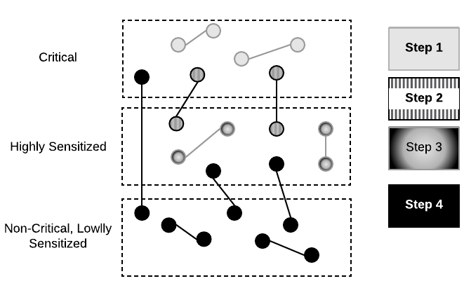
In addition to relieving stress on the branch-and-price solver by addressing smaller groups at a time, this algorithm also avoids a computationally-heavy weighting function—valid in the future, but not for immediate implementation.

5 Conclusion

Before kidney exchanges can run, they must decide on a matching rule. Where Dickerson Dickerson et al. 2014 showed that utilitarian matching rules undermine sensitized patients in static settings, we theoretically showed that sensitization-based matching rules result in patient losses in dynamic settings. We also present a new definition of fairness, lexicographical time fairness, which maximizes the matching of critically-ill, time-sensitive pairs, and we propose a batched algorithm to balance time and sensitization needs. We contribute by being one of the first to consider dynamics fairness, uniquely evaluate fairness using losses, and the first to propose a time fairness.

Our work suggests that time plays a larger role in kidney exchange than currently acknowledged. Minimizing wait times and quickly clearing critical patients likely requires more than a modification to current branch-and-price solvers; they instead require an explicitly dynamic solver. We essentially justify recent attempts to entirely reformulate static solvers into dynamic ones, especially theoretical work in the formal Markov Decision Process environment Akbarpour et al. 2014 Anderson et al. 2014. These solvers naturally optimize time fairness by weighting matches based on long-term utility with future-discounting; only sensitization fairness needs to be later imposed.

In the end, it is important to remember that kidney problems affect over a tenth of the United States population, making kidney exchange an important, and so time-pressed, innovation. Yet the care we take to design matching rules is more than theorizing; they affect the fairness, efficiency, and health of us all.

References

Abecassis et al. (2000) Michael Abecassis, Mark Adams, Patricia Adams, Robert M Arnold, and Carolyn R. Atkins. Consensus Statement on the Live Organ Donor. Journal of the American Medical Association, 284(22), December 2000.
Abraham et al. (2007) David J. Abraham, Avrim Blum, and Tuomas Sandholm. Clearing Algorithms for Barter Exchange Markets: Enabling Nationwide Kidney Exchanges. In Proceedings of the 8th ACM Conference on Electronic Commerce, EC ’07, pages 295–304, New York, NY, USA, 2007. ACM.
Akbarpour et al. (2014) Mohammad Akbarpour, Shengwu Li, and Shayan Oveis Gharan. Dynamic Matching Market Design. arXiv: 1402.3643, February 2014.
Al-Aly et al. (2010) Ziyad Al-Aly, Angelique Zeringue, John Fu, Michael I. Rauchman, Jay R. McDonald, Tarek M. El-Achkar, Sumitra Balasubramanian, Diana Nurutdinova, Hong Xian, Kevin Stroupe, Kevin C. Abbott, and Seth Eisen. Rate of Kidney Function Decline Associates with Mortality. Journal of the American Society of Nephrology : JASN, 21(11):1961–1969, November 2010.
Anderson et al. (2014) R. Anderson, I. Ashlagi, D. Gamarnik, and Y. Kanoria. A dynamic model of barter exchange. In Proceedings of the Twenty-Sixth Annual ACM-SIAM Symposium on Discrete Algorithms, pages 1925–1933, San Diego, CA, USA, December 2014. Society for Industrial and Applied Mathematics. DOI: 10.1137/1.9781611973730.129.
Ashlagi and Roth (2011) Itai Ashlagi and Alvin E. Roth. Individual Rationality and Participation in Large Scale, Multi-Hospital Kidney Exchange. Working Paper 16720, National Bureau of Economic Research, January 2011. DOI: 10.3386/w16720.
Ashlagi et al. (2013) Itai Ashlagi, Patrick Jaillet, and Vahideh H. Manshadi. Kidney Exchange in Dynamic Sparse Heterogenous Pools. arXiv: 1301.3509, January 2013.
Center (2017) Cedars-Sinai Kidney & Pancreas Transplant Center. Highly Sensitized Transplants, 2017.
Dickerson et al. (2012) John P Dickerson, Ariel D. Procaccia, and Tuomas Sandholm. Dynamic Matching via Weighted Myopia with Application to Kidney Exchange. In Proceedings of the National Conference on Artificial Intelligence, volume 2, pages 1340–1346, Toronto, ON, Canada, 2012.
Dickerson et al. (2014) John P. Dickerson, Ariel D. Procaccia, and Tuomas Sandholm. Price of Fairness in Kidney Exchange. In Proceedings of the 2014 International Conference on Autonomous Agents and Multi-agent Systems, AAMAS ’14, pages 1013–1020, Richland, SC, 2014. International Foundation for Autonomous Agents and Multiagent Systems.
Hajaj et al. (2015) Chen Hajaj, John P. Dickerson, Avinatan Hassidim, Tuomas Sandholm, and David Sarne. Strategy-Proof and Efficient Kidney Exchange Using a Credit Mechanism. In AAAI, pages 921–928, 2015.
Kahng (2016) Anson Kahng. Timing Objectives in Dynamic Kidney Exchange. PhD thesis, Harvard University, Cambridge, MA, April 2016.
Procurement et al. (2017) Organ Procurement, Transplantation Network, US Department of Health, and Human Services. National data. Technical report, 2017.
Roth et al. (2004) Alvin Roth, Tayfun Sonmez, and M. Utku Unver. Kidney Exchanges. Quarterly Journal of Economics, 119(2):457–488, May 2004.
Sumida et al. (2016) Keiichi Sumida, Miklos Z. Molnar, Praveen K. Potukuchi, Fridtjof Thomas, Jun Ling Lu, Jennie Jing, Vanessa A. Ravel, Melissa Soohoo, Connie M. Rhee, Elani Streja, Kamyar Kalantar-Zadeh, and Csaba P. Kovesdy. Association of Slopes of Estimated Glomerular Filtration Rate With Post-End-Stage Renal Disease Mortality in Patients With Advanced Chronic Kidney Disease Transitioning to Dialysis. Mayo Clinic Proceedings, 91(2):196–207, February 2016.
Unver (2010) M. Utku Unver. Dynamic Kidney Exchange. Review of Economic Studies, 77, 2010.
U.S. Renal Data System et al. (2014) National Institute of Diabetes U.S. Renal Data System, National Institutes of Health, Digestive, and Kidney Diseases. 2013 annual data report: Atlas of end-stage renal disease in the united states. Technical report, 2014.
U.S. Renal Data System et al. (2016) National Institute of Diabetes U.S. Renal Data System, National Institutes of Health, Digestive, and Kidney Diseases. 2016 usrds annual data report. Technical report, 2016.