Latent Variables on Spheres for Autoencoders in High Dimensions
Abstract
Variational Auto-Encoder (VAE) has been widely applied as a fundamental generative model in machine learning. For complex samples like imagery objects or scenes, however, VAE suffers from the dimensional dilemma between reconstruction precision that needs high-dimensional latent codes and probabilistic inference that favors a low-dimensional latent space. By virtue of high-dimensional geometry, we propose a very simple algorithm, called Spherical Auto-Encoder (SAE), completely different from existing VAEs to address the issue. SAE is in essence the vanilla autoencoder with spherical normalization on the latent space. We analyze the unique characteristics of random variables on spheres in high dimensions and argue that random variables on spheres are agnostic to various prior distributions and data modes when the dimension is sufficiently high. Therefore, SAE can harness a high-dimensional latent space to improve the inference precision of latent codes while maintain the property of stochastic sampling from priors. The experiments on sampling and inference validate our theoretical analysis and the superiority of SAE.
Keywords:
Machine Learning, ICML1 Introduction
Generative models, such as the autoencoder (Hinton & Salakhutdinov 2006) and Variational Auto-Encoder (VAE) (Kingma & Welling 2013; Rezende et al. 2014), play more and more important role for nonlinear dimensionality reduction and generation in machine learning and computer vision. The (variational) autoencoder has been a fundamental architecture of designing algorithms in deep learning. Our work will focus on the optimization of the autoencoder and make it more robust to prior distributions and the dimension of the latent space than VAE.
Formally, suppose that is a data point in the -dimensional observable space and its low-dimensional representation in the feature space , where . The general formulation of the autoencoder can be written as
| (1) |
where and are the encoder and the decoder, respectively, and is the reconstruction of . The mapping can be viewed as nonlinear dimensionality reduction and the role of as a regularizer to in the autoencoder (Hinton & Salakhutdinov 2006).
VAE improves the vanilla autoencoder by posing a stochastic condition on the variables in , such that the latent variables comply with a given prior distribution . According to convention, we let represent the latent variable. Thus we can write the diagram of VAE as
| (2) |
In the parlance of probability, the process of is called inference, and the other procedure of is called sampling or generation. VAE is capable of carrying out one-pass inference and generation in one framework by two collaborative functional modules. An elegant algorithm was proposed by (Kingma & Welling 2013) to solve VAE via variational inference. However, a limitation of VAE is that it is sensitive to the dimension of the latent space and restrictive to the prior. We will give the analysis in section 2.
Using the geometric theory in this paper, we propose a simple method to improve the autoencoder with a latent space robust to stochastic sampling and dimension. Our theory is to reshape the latent space of the autoencoder on a sphere in high dimension, i.e.
| (3) |
where is the sphere embedded in and is the all-one vector. Here we have no any probabilistic constraint on . With centerized on the sphere, we can rigorously prove that is robust to sampling on arbitrary prior distributions and varying dimensions. Our contributions are summarized as follows.
- •
The dimensional dilemma in VAE is analyzed when the dimension of the latent space is high.
- •
We introduce the volume concentration of high-dimensional spheres. Based on this property, we point out that projecting latent variable on a sphere is favorable of learning from the viewpoint of the volume in high-dimensional spaces.
- •
We further introduce the probability distribution of distances between two arbitrary sets of random latent variables on the sphere in high dimensions and illustrate the phenomenon of distance convergence. Furthermore, we prove that the Wasserstein distance between two arbitrary sets of latent variables randomly drawn from a high-dimensional sphere are nearly identical, meaning that the variables on the sphere are distribution-robust.
- •
Based on our theoretical analysis, we propose a very simple algorithm, called Spherical Auto-Encoder (SAE), to improve the vanilla autoencoder. The spherical normalization is simply put on latent variables instead of variational inference. In contrast to variational inference, we name the corresponding inference by SAE as spherical inference.
We perform the experiments on MNIST letters and FFHQ faces to validate our theoretical analysis and claims with sampling and inference.
2 Dimensional Dilemma in VAE
To be formal, we write the approximation of the marginal log-likelihood for VAE as
| (4) | ||||
| (5) |
where is the Kullback-Leibler divergence with respect to the posterior probability and the prior . This lower bound is the objective to be optimized in VAE. The variational inference is an elegant solution to learn a stochastic latent space for an autoencoder. However, this probabilistic method suffers a critical limitation when the dimension of the latent space is high.
To understand this, we need to examine VAE from a dimensional view. The encoding operation can be regarded as the process of dimensionality reduction. To correctly reconstruct through the decoder, one condition is that the dimension of the latent space is no less than the intrinsic dimension of the underlying manifold where is drawn (Tenenbaum et al. 2000; Roweis & Saul 2000; Bengio et al. 2003). Otherwise, the subspaces of the manifold will be folded after the encoder’s projection and the reconstruction information will be lost, thus leading to impossibility of precise reconstruction via the decoder. To maintain the reconstruction precision, therefore, the autoencoder requires that should not be too low. From a probabilistic view, however, a large incurs the difficulty of fitting probabilistic distributions in high-dimensional latent spaces (Scott 1992; van Handel 2016). This phenomenon is called the curse of dimensionality that can be interpreted via a simple geometric fact. The volume ratio between a cube and its inscribed sphere goes to infinity when the dimension goes very large, meaning that the data points become rather sparse in high dimensions. Actually, the number of data points needed to fit a distribution grows exponentially when the dimension increases (Scott 1992). Thus, the Kullback-Leibler divergence in (5) becomes challenging to measure the similarity between two distributions in high dimensions, provided a fixed number of data points. Therefore, is usually taken with much lower dimension compared with in VAE to void the curse of dimensionality. This is the dimensional dilemma in VAE. Our work aims to solve this problem.
| (a) Low dimension. | (b) High dimension. | (c) Distance convergence in high dimension. |
3 Latent Variables on Spheres
For latent variables sampled from some priors, the projection on the unit sphere can can be easily performed by
| (6) |
This spherical normalization for priors fed into the generator is employed in StyleGAN that is the phenomenal algorithm in GANs (Karras et al. 2018a; Karras et al. 2018b). In practice, we observe that StyleGAN with sphere-normalized is much more robust to the variation of variable modes from different distributions. Inspired by this observation, we interpret the benefit of using random variables on spheres by virtue of high-dimensional geometry in this section. Based on these geometric theories, a novel algorithm is proposed for improving autoencoder.
3.1 Volume Concentration
For high-dimensional spaces, there are many counter-intuitive phenomena that will not happen in low-dimensional spaces. For a convenient analysis, we assume that the center of the sphere embedded in is at the origin. The concentration property of sphere volume is such intriguing counter-intuitive geometry. Volume concentration says that the volume of the -dimensional sphere of radius ( ) rapidly goes to zero when goes large (Blum et al. 2020), meaning that the interior of the high-dimensional sphere is empty. In other words, nearly all the volume of the sphere is contained in the thin annulus of width . The width becomes very thin when grows. For example, the annulus of width that is of the radius contains of all the volume for the sphere in . To help understand this counter-intuitive geometric property, we make a schematic illustration in Figures 1 (a) and (b).
In fact, the distributions defined on the sphere have been already exploited to re-formulate VAE, such as the von Mises-Fisher distribution (Davidson et al. 2018; Xu & Durrett 2018). But the algorithms proposed in (Davidson et al. 2018; Xu & Durrett 2018) still fall into the category using the variational inference like the vanilla VAE, which also suffers from the dimensional dilemma. To eliminate this constraint, we need more geometric analysis.
3.2 Distance Convergence
To dig deeper, we examine the pairwise distance between two arbitrary points randomly sampled on . The following important theorem was proved by (Lord 1954; Lehnen & Wesenberg 2002).
Theorem 1.
Let denote the Euclidean distance between two points randomly sampled on the sphere of radius . Then the probability distribution of is
| (7) |
where the coefficient is given by . And the mean distance and the standard deviation are
| (8) |
respectively, where is the Gamma function. Furthermore, and when goes large.
Theorem 1 tells that the pairwise distances between two arbitrary points randomly sampled on approach to be mutually identical and converge to the mean when grows. The associated standard deviation . We display the average distance and its standard deviation in Figure 1(c), showing that the convergence process is fast. Taking for example, we calculate that and . The standard deviation is only of the average distance, meaning that the distance discrepancy between two arbitrary and on the sphere is rather small. This surprising phenomenon is also observed for neighborly polytopes when solving the sparse solution of underdetermined linear equation (Donoho 2005) and for nearest neighbor search in high dimensions (Beyer et al. 1999).
With Theorem 1, we can study the property of two different random datasets on pertaining to distribution-free sampling and spherical inference in generative models. Let and be the datasets of random variables drawn from at random, respectively. Our goal is to investigate the influence of two arbitrary different groups of latent variables on the autoencoder. A rigorous way of quantifying the discrepancy between two datasets is the Wasserstein distance. To this end, we introduce the computational definition of -Wasserstein distance as
| (9) | ||||
| (10) |
where is the doubly stochastic matrix. Then we have
Corollary 1.
with zero standard deviation when .
Corollary 1 says that despite the diverse data modes, the -Wasserstein distance between two arbitrary sets of random variables randomly drawn on the sphere converges to a constant when the dimension is sufficiently large. For generative models, this unique characteristic brings great convenience for distribution-robust sampling and spherical inference. For example, if and obeys the different distributions, the functional role of nearly coincides with that of with respect to Wasserstein distance, provided that both and are randomly drawn from the high-dimensional sphere. The specific distributions of and affect the result negligibly under such a condition. We will present the specific application of Corollary 1 in the following section.
In fact, we can obtain the bounds of using the proven proposition about the nearly-orthogonal property of two random points on high-dimensional spheres (Cai et al. 2013). However, Corollary 1 is sufficient to solve the problem raised in this paper. So, we bypass this analysis to simplify the theory for easy readability.
3.3 Variable Centerization
Both Theorem 1 and Corollary 1 hold under one critical condition that latent vectors are randomly drawn from the sphere. In practice, however, this randomness for real data is hard to satisfy. For example, the condition violates if is sampled from the open positive orthant and from the open negative orthant, or from the normal distribution and from the Chi-squared distribution, etc. Hopefully, we can resort to central limit theorem to deal with it. For an arbitrary random vector , we let and the mean . Assume that is independent, identically distributed variables. Central limit theorem says that (Billingsley 1995)
| (11) |
when is sufficiently large. This conclusion is very meaningful for our case because the distribution of the mean can be the standard normal one despite the distribution of variable . To satisfy the condition in Theorem 1 and Corollary 1, therefore, a very simple approach is that we only need to normalize latent variables by centerization and spherization , on which is based our algorithm of spherical autoencoder that is prior-agnostic.
4 Spherical Autoencoder
According to Theorem 1, we may know that latent variables is agnostic to diverse distributions if they are randomly sampled from the high-dimensional sphere. Volume concentration guarantees that the error can be negligible even if they deviate from the sphere, as long as they are scattered near the spherical surface. This tolerance to various modes of latent random variables allow us to devise a simple solution to replace the variational inference for VAE. To be specific, we only need to constrain the centerized latent variables on the sphere by means of the standard framework of an autoencoder, as opposed to the conventional way of employing the KL-divergence or its variants with diverse priors. We can write the objective function for spherical autoencoder as
| (12) | ||||
| s.t. | (13) |
where denotes the -norm, , and . The constraint in (13) can be fulfilled with spherical normalization, which is shown in the following the sequential mappings of the SAE framework
| (14) |
where is the average of elements in . The objective function and the framework of our algorithm are much simpler than that of VAE and hyper-spherical VAE based on the variational inference or the variants of VAEs that apply various sophisticated regularizers on latent spaces. Our algorithm is purely geometric and free from the difficulty of any probability optimization.
5 Related work
Little attention has been paid on examining geometry of latent spaces in the field of generative models. So we find few works directly related to ours. Most relevant one is S-VAE (Davidson et al. 2018; Xu & Durrett 2018), which applies the von Mises-Fisher (vMF) distribution as the probability prior. The vMF distribution is defined on the sphere. The algorithms proposed in (Davidson et al. 2018; Xu & Durrett 2018) both rely on the variational inference as VAE does. Therefore, S-VAE also suffers the dimensional dilemma and is restricted by specific priors.
From the sampling viewpoint, our geometric analysis is directly inspired by ProGAN (Karras et al. 2018a) and StyleGAN (Karras et al. 2018b) that have already applied spherical normalization (i.e. equation (6)) for sampled inputs. We study the related theory and extend the case to devise a novel autoencoder that is free from the dimensional dilemma and is prior-agnostic. Another related method is to sample priors along the great circle when performing the interpolation in the latent space for GANs (White 2016). This algorithm is perfectly compatible with our theory and algorithm. Therefore, it can also be harnessed in our algorithm when performing interpolation as well.
Wasserstein Auto-Encoder (WAE) (Tolstikhin et al. 2018) is an alternative way of optimizing the model distribution and the prior distribution using Wasserstein distance. Different from WAE, SAE does not really use Wasserstein distance in the latent space. We just leverage Wasserstein distance to establish Corollary 1 for the theoretical analysis. Adversarial Auto-Encoder (AAE) (Makhzani et al. 2015) is another interesting method of replacing the variational inference with adversarial learning in the latent space. But both WAE and AAE need some priors to match, which are essentially different from SAE.
Spherical Normalization (SN) in (14) is easily reminiscent of Batch Normalization (BN) (Ioffe & Szegedy 2015) widely applied in deep learning. BN is performed among a batch of data points and there are learnable parameters, such that the normalization on data by BN relys on data modes or distributions. However, SN manipulates a single data point, independent of data distributions. Central limit theorem and Theorem 1 guarantee its plausibility. So SN and BN are established on different theory and for different purpose.
6 Experiment
We conduct the experiments to test our theory and algorithms in this section. Three aspects pertaining to generative algorithms are taken into account, including sampling GANs, learning the variants of autoencoder, and sampling the decoders.
The MNIST and FFHQ datasets are used to evaluate algorithms. FFHQ (Karras et al. 2018b) is a more complex face dataset with large variations of faces captured in the wild. We use the image size of , which is larger than the commonly chosen size in the related work and also more challenging than or for (variational) autoencoders to reconstruct. We test VAE and our SAE algorithm with this benchmark dataset for the case of high dimensions.
6.1 Sampling GAN
Our first experiment is to validate our theory and the robustness of our algorithm against diverse distributions for sampling. We employ StyleGAN trained with random variables sampled from the normal distribution. The other three different distributions are opted to test the generation with different priors after training, i.e. the uniform, Poisson, and Chi-squared distributions. The shapes of these three distributions are significantly distinctive from that of the normal distribution. Thus, the generalization capability of the generative models can be effectively unveiled when fed with priors that are not involved during training. We follow the experimental protocol in (Karras et al. 2018a; Karras et al. 2018b) that StyleGAN is trained on the FFHQ face dataset and Fréchet inception distance (FID) (Borji 2018) is used as the quality metrics of generative results. We take , which is set in StyleGAN. This dimension is also used for both VAE and SAE on face data.
From Table 1, we can see that the generative results by the normal distribution is significantly better than the others when tested with the original samples. The uniform distribution is as good as the normal distribution when projected on the sphere. This is because the values for each random vector are overall symmetrically distributed according to the origin. They satisfy the condition in Corollary 1 after the spherical projection. The accuracy of Poisson and Chi-squared distributions is considerably improved after centerization, even better than the vanilla uniform distribution. But the accuracy difference between all the compared distributions is rather negligible after centerization and spherization, empirically verifying the theory presented in Corollary 1 and the distribution-agnostic property of our algorithm.
| no centerization | centerization | |||
|---|---|---|---|---|
| Distribution | no sph | sph | no sph | sph |
| Normal | 6.20 | 6.16 | 6.27 | 6.12 |
| Uniform | 33.93 | 6.16 | 33.86 | 6.16 |
| Poisson | 23.70 | 26.85 | 18.15 | 6.19 |
| Chi | 25.26 | 27.07 | 11.34 | 6.16 |
 |
 |
 |
 |
| (a) MNIST samples | (b) VAE | (c) S-VAE | (d) SAE (ours) |
| (a) VAE (normal) | (b) S-VAE (von Mises-Fisher) | (c) SAE (ours) |
| VAE | S-VAE | SAE (ours) |
 |
 |
 |
| Normal distribution | ||
 |
 |
 |
| Uniform distribution | ||
 |
 |
 |
| Poisson distribution | ||
 |
 |
 |
| Chi-squared distribution |
6.2 MNIST Letters
We now use the commonly used MNIST dataset to learn the autoencoders of different styles, i.e. VAE, S-VAE, and our SAE. For all experiments on MNIST, we take .
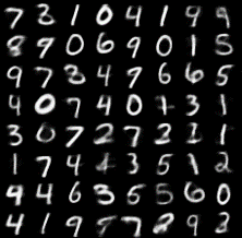
From Figure 2, we can see that the reconstruction letters by SAE are more faithful to the original ones than VAE and S-VAE. For example, both VAE and S-VAE fail to recover the second letter “2” in the first row for each sub-figure while SAE obtains the accurate reconstruction. To further reveal the advantage of SAE, we visualize the latent codes of letters in Figure 3 with t-SNE (van der Maaten & Hinton 2008). It is clear that the latent codes derived from SAE are much better than that from VAE and S-VAE. The margins between different classes are wider, meaning that the latent codes from the spherical inference conveys more discriminative information in the way of unsupervised learning. This experiment also indicates that SAE captures the intrinsic structure of multi-class data better than VAE and S-VAE.
The superiority of SAE is more obvious when sampling the decoders after training, as Figure 4 shows. For VAE, the sampling results from normal and uniform distributions are blurry and the mode aggregation occurs for Poisson and Chi-squared distributions. For S-VAE, the sampling letters are worse than the reconstruction in Figure 2, implying that S-VAE is sensitive to priors. As a comparison, SAE performs consistently well on four priors, validating its robustness to different distributions and data modes.
| FFHQ faces |  |
|---|---|
| VAE |  |
| SAE |  |
| VAE | SAE (ours) |
 |
 |
| Normal distribution | |
 |
 |
| Uniform distribution | |
 |
 |
| Poisson distribution | |
 |
 |
| Chi-squared distribution | |
| Metric | FID | SWD | MSE |
|---|---|---|---|
| VAE | 134.22 | 77.68 | 0.091 |
| SAE (ours) | 91.02 | 56.58 | 0.063 |
VAE  |
SAE  |
6.3 FFHQ faces
We compare the vanilla VAE with the normal prior (Kingma & Welling 2013) with our SAE algorithm for reconstruction and sampling tasks on face data in this section. S-VAE is not compared because we fail to train S-VAE on the FFHQ dataset From Figure 5, we can see that the face quality of SAE outperforms that of VAE. The imagery details like semantic structures are preserved much better for SAE. For example, the sunglasses in the sixth image is successfully recovered by SAE, whereas VAE distorts the face due to this occlusion. It is worth emphasizing that the blurriness for images reconstructed by SAE is much less than that by VAE, implying that the spherical inference is superior to the variational inference in VAE. The different accuracy measurements in Table 2 also indicate the consistently better performance of SAE.
To test the generative capability of the models, we also perform the experiment of sampling the decoders as done in section 6.1. Prior samples are drawn from the normal, uniform, Poisson, and Chi-squared distributions, respectively, and then fed into the decoders to generate faces. Figure 6 illustrates the generated faces of significantly different quality with respect to four types of samplings. The style of the generated faces by SAE keeps consistent, meaning that SAE is rather robust to different probability priors. This also empirically verifies the correctness of Theorem 1 by solving the real problem. As a comparison, the quality of the generated faces by VAE varies with probability priors. In other words, VAE is sensitive to the outputs of the encoder with the variational inference, which is probably the underlying reason of the difficulty of training VAE with sophisticated architectures. We also present the experimental results on CelebA in supplementary material.
6.4 Varying Latent Dimensions
To investigate the effectiveness of SAE to circumvent the dimensional dilemma, we analyze the results of varying the dimension of the latent spaces for VAE and SAE. As shown in Figure 8, SAE is capable of monotonically decreasing the reconstruction error when the latent dimension grows. As a comparison, VAE’s reconstruction error begins to increase when the dimension is larger than 512, meaning that the curse of dimensionality occurs. For VAE, the latent codes of faces beyond 512 dimensions are too high to be applicable for variational inference. It is also obvious that the high latent codes of SAE produce significantly better performance than that of VAE, implying that the potential capability of the autoencoder can be unlocked if the curse of dimensionality posed on the latent random space can be eliminated. Figure 7 illustrates that the reconstructed faces by SAE are consistently better than that by VAE. More examples are attached in supplementary material.
7 Conclusion
In this paper, we attempt to address the curse of dimensionality for VAE. By analyzing the geometry of volume concentration and distance convergence on the high-dimensional sphere, we prove that the Wasserstein distance converges to be a constant for two datasets randomly sampled from the sphere when the dimension goes large. These unique characteristics imply that two random datasets drawn on the high-dimensional sphere are distribution-agnostic. Based on this theory, we propose a very simple algorithm called Spherical Auto-Encoder (SAE). SAE is a standard autoencoder with spherical normalization on the latent space. The experiments on the MNIST letter and FFHQ face databases validate the effectiveness of our theory and new algorithm for sampling and spherical inference.
It is worth noting that the applications of our theory and algorithm are not limited for autoencoders. Interested readers may explore the possibility in other scenarios.
References
- Bengio et al. (2003) Bengio, Y., Paiement, J.-F., Vincent, P., Delalleau, O., Roux, N. L., and Ouimet, M. Out-of-sample extensions for LLE, Isomap, MDS, Eigenmaps, and spectral clustering. In Advances in Neural Information Processing Systems (NeurIPS), pp. 177–184, 2003.
- Beyer et al. (1999) Beyer, K., Goldstein, J., Ramakrishnan, R., and Shaft, U. When is “nearest neighbor” meaningful? In International Conference on Database Theory, pp. 217–235, 1999.
- Billingsley (1995) Billingsley, P. Probability and Measure. Wiley, 1995.
- Blum et al. (2020) Blum, A., Hopcroft, J., and Kannan, R. Foundations of Data Science. Cambridge University Press, 2020.
- Borji (2018) Borji, A. Pros and cons of GAN evaluation measures. arXiv:1802.03446, 2018.
- Cai et al. (2013) Cai, T., Fan, J., and Jiangd, T. Distributions of angles in random packing on spheres. Journal of Machine Learning Research, 4:1837–1864, 2013.
- Davidson et al. (2018) Davidson, T. R., Falorsi, L., Cao, N. D., Kipf, T., and Tomczak, J. M. Hyperspherical variational auto-encoders. In Proceedings of the Thirty-Fourth Conference on Uncertainty in Artificial Intelligence (UAI), 2018.
- Donoho (2005) Donoho, D. L. Neighborly polytopes and sparse solutions of underdetermined linear equations. Technical report, Stanford University, 2005.
- Hinton & Salakhutdinov (2006) Hinton, G. E. and Salakhutdinov, R. R. Reducing the dimensionality of data with neural networks. Science, 313(5786):504–507, 2006.
- Ioffe & Szegedy (2015) Ioffe, S. and Szegedy, C. Batch normalization: Accelerating deep network training by reducing internal covariate shift. In International Conference on Machine Learning, pp. 448–456, 2015.
- Karras et al. (2018a) Karras, T., Aila, T., Laine, S., and Lehtinen, J. Progressive growing of GANs for improved quality, stability, and variation. In Proceedings of the 6th International Conference on Learning Representations (ICLR), 2018a.
- Karras et al. (2018b) Karras, T., Laine, S., and Aila, T. A style-based generator architecture for generative adversarial networks. arXiv:1812.04948, 2018b.
- Kingma & Welling (2013) Kingma, D. P. and Welling, M. Auto-encoding variational bayes. In Proceedings of the 2th International Conference on Learning Representations (ICLR), 2013.
- Lehnen & Wesenberg (2002) Lehnen, A. and Wesenberg, G. The sphere game in n dimensions. 2002. http://faculty.madisoncollege.edu/alehnen/sphere/hypers.htm.
- Lord (1954) Lord, R. D. The distribution of distance in a hypersphere. The Annals of Mathematical Statistics, 25(4):794–798, 1954.
- Makhzani et al. (2015) Makhzani, A., Shlens, J., Jaitly, N., Goodfellow, I., and Frey, B. Adversarial autoencoders. arXiv:1511.05644, 2015.
- Rezende et al. (2014) Rezende, D. J., Mohamed, S., and Wierstra, D. Stochastic backpropagation and approximate inference in deep generative models. In International Conference on Machine Learning (ICML), pp. 1278–1286, 2014.
- Roweis & Saul (2000) Roweis, S. T. and Saul, L. K. Nonlinear dimensionality reduction by locally linear embedding. Science, 290(5500):2323–2326, 2000.
- Scott (1992) Scott, D. W. Multivariate Density Estimation: Theory, Practice, and Visualization. Wiley, 1992.
- Tenenbaum et al. (2000) Tenenbaum, J. B., de Silva, V., and Langford, J. C. A global geometric framework for nonlinear dimensionality reduction. Science, 290(5500):2319–2323, 2000.
- Tolstikhin et al. (2018) Tolstikhin, I., Bousquet, O., Gelly, S., and Schoelkopf, B. Wasserstein auto-encoders. In International Conference on Learning Representations (ICLR), 2018.
- van der Maaten & Hinton (2008) van der Maaten, L. and Hinton, G. Visualizing high-dimensional data using t-SNE. Journal of Machine Learning Research, 9:2579–2605, 2008.
- van Handel (2016) van Handel, R. Probability in High Dimension. Princeton University, 2016.
- White (2016) White, T. Sampling generative networks. arXiv:1609.04468, 2016.
- Xu & Durrett (2018) Xu, J. and Durrett, G. Spherical latent spaces for stable variational autoencoders. In Conference on Empirical Methods in Natural Language Processing (EMNLP), 2018.
Appendix A Reconstruction on FFHQ

Appendix B Sampling VAE and SAE on FFHQ
 |
 |
Appendix C Reconstruction on CelebA
 |
Appendix D Sampling on CelebA
 |
Appendix E Visualization of Inference
| (a) VAE |
| (b) SAE (ours) |
Appendix F Reconstructed Faces with Dimension Growing
VAE
SAE