∎
A Region-based Randers Geodesic Approach for Image Segmentation
Abstract
The geodesic model based on the eikonal partial differential equation (PDE) has served as a fundamental tool for the applications of image segmentation and boundary detection in the past two decades. However, the existing approaches commonly only exploit the image edge-based features for computing minimal geodesic paths, potentially limiting their performance in complicated segmentation situations. In this paper, we introduce a new variational image segmentation model based on the minimal geodesic path framework and the eikonal PDE, where the region-based appearance term that defines then regional homogeneity features can be taken into account for estimating the associated minimal geodesic paths. This is done by constructing a Randers geodesic metric interpretation of the region-based active contour energy functional. As a result, the minimization of the active contour energy functional is transformed into finding the solution to the Randers eikonal PDE.
We also suggest a practical interactive image segmentation strategy, where the target boundary can be delineated by the concatenation of several piecewise geodesic paths. We invoke the Finsler variant of the fast marching method to estimate the geodesic distance map, yielding an efficient implementation of the proposed region-based Randers geodesic model for image segmentation. Experimental results on both synthetic and real images exhibit that our model indeed achieves encouraging segmentation performance.
Keywords:
Region-based active contours minimal geodesic path Randers metric image segmentation Finsler variant of the fast marching method eikonal partial differential equation1 Introduction
1.1 Related Work
Active contour models are commonly established upon the mathematical frameworks of PDE, energy minimization and numerical analysis, thus featuring a quite solid theoretical background. These models are able to take advantage of efficient geometry priors and reliable image features to design flexible energy functionals, whose minimizers yield suitable solutions to a great variety of image segmentation tasks.
The classical snakes model (Kass et al 1988) can be regarded as one of the earliest active contour approaches, which rely on continuous curves to delineate image edges of interest. In its basic formulation, active curves move and deform according to an internal regularization force and an image external force, both of which are derived from the Euler-Lagrange equation of an energy functional. Great efforts have been devoted to improvements of the classical snakes model so as to obtain satisfactory solutions in various image segmentation scenarios. However, an important shortcoming of the classical snakes model is its sensitivity to the curve initialization. One possible way to overcome this issue is to design new external force fields with sufficiently large capture range. Significant examples along this research line may involve the approaches introduced in (Cohen 1991; Cohen and Cohen 1993; Xu and Prince 1998; Jalba et al 2004; Xie and Mirmehdi 2008; Li and Acton 2007). In contrast to the classical snakes model which is non-intrinsic, geodesic active contour models (Caselles et al 1997; Yezzi et al 1997; Melonakos et al 2008) make use of intrinsic energy functionals, in the sense that they are independent of the curve parametrization. In addition, these intrinsic functionals only involve to the first-order derivative of the curves, and sometimes their curvature as well using recent techniques introduced by Mirebeau 2018. On the negative side this simplification limits the expressive power of the model, but on the positive side it allows for an efficient and global minimization of the energy functionals, as discussed in (Osher and Sethian 1988; Goldenberg et al 2001; Ma et al 2021). One essential common point of the active contour models reviewed above is that they only make use of locally-defined edge-based features, usually derived from the gradient of the processed image, to build the energy functionals. While these features are effective and easy to extract, their local nature increases the risk of finding segmentations corresponding to unexpected local minima of the energy functional. Comparing to the local edge-based features, the regional appearance models are capable of penalizing the global homogeneity of the image data in each subregion.
The region-based active contour models differ from the edge-based approaches by the use of image regional appearance models, thus are insensitive to local spurious edges, for instance, generated by image noise. A pioneering region-based active contour approach is the Mumford-Shah piecewise smooth model (Mumford and Shah 1989), whose prior is that the image appearance data (e.g. gray levels or colors) can be well approximated by a piecewise smooth data-fitting function. Since then, the Mumford-Shah model has motivated a series of research works on active contour models, for instances (Vese and Chan 2002; Tsai et al 2001; Duan et al 2015; Doğan et al 2008; Zhang and Lui 2021). Among them, the approaches which impose different regional appearance priors are able to handle more complicated image segmentation issues. The region competition model (Zhu and Yuille 1996) and its generalized variant (Brox and Cremers 2009) interpreted the Mumford-Shah energy functional in a Bayes framework, by assuming that the image gray levels follow a parameter-dependent probability distribution function (PDF). In practice, the Gaussian distributions are very often chosen to model the image data within each subregion. Approaches (Chan and Vese 2001; Cohen 1997) applied with a piecewise constant appearance constraint on image data are considered as a practical reduction of the original Mumford-Shah model. From the viewpoint of statistics, these piecewise constant reduction models can also be treated as an instance of the region competition model (Zhu and Yuille 1996), with a particular assumption that image gray levels in different subregions can be modeled by Gaussian distributions of identical variance.
Nonparametric active contour models (Ni et al 2009; Michailovich et al 2007; Houhou et al 2009) usually construct the energy functional by measuring the statistical distances between the histograms of the image data in different subregions, thus allowing to work in the absence of prior knowledge on the image data distribution. In (Kimmel 2003; Bresson et al 2007; Jung 2017), the -norm was taken into account for measuring the approximation errors between the image data and the fitting terms. Active contour approaches based on the pairwise homogeneity criteria are capable of successfully handling more complicated segmentation situations (Sumengen and Manjunath 2006; Bertelli et al 2008; Jung et al 2012; Bresson and Chan 2008; Desquesnes et al 2013), but the estimation of the associated gradient descent flows has a high computational complexity. Hybrid active contour models simultaneously integrate the region-based image appearance models and the edge-based features (Paragios and Deriche 2002; Kimmel and Bruckstein 2003; Zach et al 2009; Bresson et al 2007; Chen et al 2021b) for building the energy functionals, so as to cumulate the benefits of both types of features. The segmentation models in conjunction with prescribed shape constraints (e.g. statistical shape priors, convexity and star convexity shape priors) have proven to generate accurate segmentation results (Cremers et al 2002; Bresson et al 2006; Chen et al 2022; Chen et al 2021a; Shi and Li 2021; Siu et al 2020; Luo et al 2022; Zhang et al 2021; Prevost et al 2014), especially for the case that the features derived from the image data are not reliable enough. In (Sundaramoorthi et al 2007; Sundaramoorthi et al 2009; Yang and Sundaramoorthi 2015), the curve evolution is driven by a type of Sobolev gradient flows, allowing imposing various flexible geometry priors to enhance the image segmentation process.
Level set formulations (Osher and Sethian 1988) represent a closed curve by means of the zero-level line of a scalar-valued function (e.g. signed Euclidean distance map to the curve), which is considered as a quite effective solution to the contour evolution problems (Cremers et al 2007; Dubrovina-Karni et al 2015; Brox and Weickert 2006; Li et al 2008; Zhang et al 2019; Alvarez et al 2018). However, the active contour models relying on the level set schemes often suffer from numerical difficulties in practical segmentation applications, due to the non-convex nature of the associated energy functionals. The approaches (Chan et al 2006; Bresson et al 2007; Chambolle et al 2012; Bae and Tai 2011; Yuan et al 2014) based on a convex relaxation of the level set method allow finding the global minimum of a region-based active contour energy reformulated in a convex set, thus are less demanding on initialization, and also benefit from efficient numerical techniques for convex optimization. Instead of working with the PDE framework, graph-based optimization algorithms have been exploited to address various active contour problems (Boykov and Kolmogorov 2003; Grady and Alvino 2009; Mishra et al 2011).

1.2 Optimal Paths-based Image Segmentation Approaches
In geodesic active contour models (Caselles et al 1997; Yezzi et al 1997), the minimization of the energy (i.e. the cost of paths) is implemented through a curve evolution scheme in a gradient descent manner. Unfortunately, there is no guarantee for these approaches to find the globally minimizing curves. In order to address this issue, Cohen and Kimmel 1997 introduced a minimal path model whose global minimizer can be extracted from the solution to a nonlinear eikonal PDE. The energy of this model is defined as the Euclidean length of the path modulated by a local positive coefficient. The scope of this approach was later extended to encompass energies defined by a Riemannian or a Finslerian metric, allowing to favor paths aligned with certain directions and orientations in an anisotropic manner (Melonakos et al 2008; Bougleux et al 2008; Chen et al 2021c), and to degenerate sub-Riemannian and sub-Finslerian metrics which can take path curvature into account (Chen et al 2017; Duits et al 2018; Mirebeau 2018). Minimal geodesic paths are a basic tool for image segmentation (Peyré et al 2010), involved in a great variety of algorithms which benefit from the efficient numerical solvers of the eikonal PDE (Sethian 1999; Mirebeau 2014b; Mirebeau 2019), and from the global optimality of the paths extracted from its solution.
In the classical geodesic models, the extraction of a minimal geodesic path requires a pair of fixed points, which serve as its endpoints. In the eikonal PDE framework, one endpoint is used as the source point defining the boundary condition of the eikonal PDE, and the other is the target point, which initializes the geodesic backtracking ordinary differential equation (ODE). Cohen and Kimmel 1997 suggested a saddle point method for image segmentation using a single source point. Taking the saddle point as the target point, one can track two geodesic paths which connect to the source point from different ways. This saddle point-based strategy is then extended in (Mille et al 2015; Cohen 2001) to closed contour detection in the scenario of multiple landmark points as source points. Accordingly, the objective contours are generated using the concatenation of a family of piecewise geodesic paths, thus passing through all given points. Benmansour and Cohen 2009 proposed an iterative keypoints sampling scheme for generating minimal paths from a single source point. In each iteration, a new keypoint is treated as a target point, form which a geodesic path can be backtracked until another keypoint is reached. Chen et al 2017 proposed to connect a set of prescribed points of unknown order through the curvature-penalized geodesic paths. These paths are tracked in an orientation-lifted space and are derived using the image boundary features extracted by a steerable filter. A common feature of the geodesic approaches mentioned above is to build the segmentation contours as the concatenation of piecewise geodesic paths. Alternatively, Appleton and Talbot 2005 introduced a circular geodesic model with a particular topology constraint, extracting a single closed geodesic path with an identical source and target point.
In contrast to geodesic models which solve the eikonal PDE to track optimal paths as segmentation contours, a crucial point for discrete paths-based models (Falcão et al 2000; Miranda et al 2012; Boykov and Kolmogorov 2003; Windheuser et al 2009) is to map the processed image to a regular graph of nodes and edges, where a discrete shortest path comprised of finite ordered nodes can be efficiently computed by the well-established graph-based optimization algorithms (Dijkstra 1959; Falcao et al 2004; Boykov and Kolmogorov 2004).
Most of the existing optimal paths-based segmentation models, using either the eikonal PDE framework or the graph-based optimization schemes, only leverage edge-based features such as image gradient features to construct the local geodesic metrics. Therefore, the resulting minimal geodesic paths in essence fall into the image edge-driven limitation, despite their possible combination with region-based homogeneity features for image segmentation as introduced in (Mille et al 2015; Appia and Yezzi 2011). Unfortunately, geodesic paths derived from the image edge-based features sometimes fail to accurately depict the boundaries of interest, especially when the processed images involve complex structures or when the image gradients are not reliable. In this paper, we introduce a region-based Randers geodesic path model for addressing the problems of active contours and image segmentation. In our model, the considered local geodesic metrics are an instance of Finslerian geometry which are constructed in terms of a region-based appearance model, i.e. regional homogeneity features, and/or anisotropic edge-based features.
In Fig. 1, we take the combination of piecewise geodesic paths model proposed by Mille et al 2015 as an example to illustrate the limitations of using edge-driven geodesic paths for segmentation. This model is an interactive segmentation method, for which a set of ordered vertices or landmark points on the target boundary should be provided. In Fig. 1a, we show the original image with four landmark points, displayed as red dots, lying on the objective boundary. One of the crucial points for the combination of piecewise geodesic paths model is the construction of a potential used for estimating the geodesic distance maps. In Fig. 1b, we show the segmentation contour (visualized by blue lines) from the combination of piecewise geodesic paths model. Clearly, some portions of the desired boundary are not extracted, and the underlying reason is that these missed boundaries are not well characterized by the edge-based features. In contrast, the geodesic paths derived from the proposed geodesic model, which blends the benefits of both region-based and edge-based features, follow the desired boundary, as illustrated in Fig. 1c.
1.3 Contribution and Paper Outline
Overall, the main contribution in this paper is threefold:
- -
Firstly, we introduce a new geodesic model which bridges the gap between the region-based active contours which involve a regional image appearance term, and the geodesic paths based on the eikonal PDE framework. The proposed model, named region-based Randers geodesic model, is an instance of Finslerian geometry, which relies on minimal geodesic paths with respect to an asymmetric Randers metric.
- -
Secondly, we present a convergence analysis of the contour evolution scheme which is proposed in this paper. We also discuss the numerical implementation of scheme, whose iterations involve the solution to a Randers eikonal PDE and to a curl PDE.
- -
Finally, we introduce a landmark points-based scheme to apply the proposed region-based Randers geodesic model to interactive image segmentation. The core idea is to extract the target boundary as a concatenation of minimal geodesic paths. Each geodesic path connects a pair of landmark points.
The manuscript is organized as follows. In Section 2, we briefly introduce the minimal path models and the corresponding Eikonal PDEs and geodesic backtracking ODEs, including the Riemannian cases and the asymmetric Randers case. Preliminary results on the hybrid active contour energy functionals and on the iterative minimization scheme for these functionals are presented in Section 3. In particular we transform in Section 3.3 the hybrid active contour energy functional into a weighted curve length associated to a Randers metric. This transformation relies on the solution to a divergence equation. In Section 4, we introduce two methods to exploit the constructed Randers metrics and the associated minimal paths for the application of image segmentation. The numerical implementation details and the experimental results are presented in Sections 5 and 6, respectively. The conclusion can be found in Section 7.
The preliminary short versions of this work were first presented in the conferences (Chen et al 2016; Chen and Cohen 2017), upon which more contributions such as the theoretical convergence analysis have been added.
2 Background on Randers Minimal Geodesic Paths
In this section, we introduce the background on the computation of paths minimizing a length defined by a Randers geodesic metric.
Notations.
We denote by a connected open bounded domain, with a smooth boundary. Points are denoted , vectors , and co-vectors . The Euclidean scalar product and norm on are denoted by and . For any we denote by the counter-clockwise orthogonal vector.
We denote by the set of symmetric positive definite matrices of shape , and we associate to each the norm . Note that , where denotes the spectral norm (i.e. the largest eigenvalue, for a symmetric positive matrix).
We denote by the set of Lipschitz functions from a metric space to another . For such a function we denote by the smallest constant such that for all . Note that a function defined over a compact space is Lipschitz iff it is locally Lipschitz.
Throughout the document, the wording “curve” refers to a parametrized curve, also known as a path. (This is in opposition to the concept of geometrical curve, not considered here, which is defined as an equivalence class of paths modulo reparametrizations.)
2.1 Randers Geodesic Metric
Randers geometry is a generalization of Riemannian geometry, and a special case of Finslerian geometry (Randers 1941; Bao et al 2012). In the general framework of path-length geometry, the energy of a path reads
| (1) |
where is the geodesic metric. Note that is well defined as an element of by Rademacher’s theorem. The energy (1) is also known as the length associated to the geodesic metric . The geodesic distance between two points is defined as the length of the shortest path joining them
| (2) | ||||
Randers geodesic metrics have, by assumption, the following structure (Randers 1941): for all ,
| (3) |
A Randers metric thus involves a positive definite tensor field , similarly to the Riemannian setting. In addition, a Randers metric features a linear term defined by a vector field , which is subject to the compatibility assumption for all . Because of this second term, a Randers metric is in general asymmetric: more precisely, whenever . As a result, the corresponding path length and geodesic distances are also asymmetric: in general and .

Minimal geodesics.
Let us briefly justify the existence of a minimizer to (2), referred to as a minimal geodesic from to , since variants of this classical argument, see the references at the end of this paragraph, are used in the mathematical analysis of our model Section 3. The two main ingredients are the Arzelà-Ascoli theorem, and the lower-semi continuity of the length functional. The former states that the set
| (4) |
equipped with which is the distance associated to uniform convergence, is compact for any compact metric spaces and and any constant . The latter affirms that, for any sequence of curves converging uniformly as , for some , one has
| (5) |
Now regarding the minimal geodesic problem (2), our assumptions on the domain (namely openness, connectedness, boundedness, smooth boundary, as stated in the notations of Section 2), imply that there exists at least one Lipschitz path from to . Denote by a sequence of paths such that , , and as . Without loss of generality, we can assume that these paths are parametrized at constant speed w.r.t. the Euclidean metric, and thus is bounded, where the constant is defined below in Eq. (6). By the Arzelà-Ascoli theorem (4), applied to and , there exists a subsequence converging uniformly as , and the limiting curve is also Lipschitz. By the lower-semi-continuity of , the limiting curve is a minimal geodesic.
A generalization of the above proof can be found in (Burago et al 2022, Section 2.5). The fact that length by integral of velocity (1) equals length by total variation is proved in (Younes 2019, Proposition 1.7), and this implies the lower semi-continuity of the length (Burago et al 2022).
Anisotropy ratios, and duality.
One often needs to compare the (possibly asymmetric) norm defined by a Randers metric at a given point , with the standard Euclidean norm . For that purpose, we introduce the minimum and maximum ratios
| (6) |
By positive homogeneity of , one has for all . The anisotropy ratio is defined as . By convention, we also set
Another object of interest is the dual norm, defined as
| (7) |
for all . The dual norm plays a central role in the generalized eikonal PDE obeyed by the distance map, and in geodesic backtracking ODE, see Section 2.2. The following result, which concludes this subsection, provides estimates of the ratios (6), sharp up to a factor two, as well as the explicit form of the dual (7) of a Randers metric.
Proposition 1
Let and be such that . Define for all . Then is definite, positively homogeneous, and obeys the triangular inequality.
The dual norm (7) has the same structure: , where , , and
The anisotropy ratios obey
| (8) | ||||
| (9) |
and thus . Also and .
The rest of this section is devoted to the proof. The positive homogeneity , and the triangular inequality , for all and , follow from the same properties of the norm and of the linear form . One has
by the Cauchy-Schwartz inequality, and therefore
| (10) |
showing that is definite, i.e. whenever . On the other hand, observing that , we find that the compatibility condition is necessary for definiteness of . Also as announced in the last sentence of the proposition.
Denote by the largest eigenvalue of , and by the corresponding unit eigenvector. One has , hence . On the other hand, the equation (10) yields as announced in Eq. (8). Conversely, if is the smallest eigenvalue of , and if is the associated eigenvector, then , hence as announced in the last sentence of the proposition.
The dual norm is given11 1 Randers norms are presented in Mirebeau 2014b with the convention corresponding to . in (Mirebeau 2014b, Proposition 4.1) by and . On the other hand, the block matrix has a non-singular top left block and Schur complement , hence its inverse is known explicitly (Lu and Shiou 2002). Comparing these expressions we obtain the announced expression of the dual norm, and also that , which alternatively could be proved in a more general setting using convex duality theory. Since is definite, one must have .
Consider . If , then , and inserting this estimate in (7) yields
hence . On the other hand, assume that and take , which satisfies , in Eq. 7. Then we obtain , hence . Exchanging the roles of the primal norm and of the dual norm leads to
hence
as announced in Eqs. (8) and (9). Thus Eq. (8) is established, and Eq. (9) follows by duality. Taking the ratio of these estimates yields the announced bounds for , which concludes the proof.
2.2 Characterization of Randers Distances and Geodesics
The framework of optimal control (Bardi and Capuzzo-Dolcetta 2008) allows characterizing the Randers geodesic distance from a given source point as the viscosity solution to an eikonal PDE. This paves the way for the numerical computation of this distance, which is presented in Section 2.3. Once the geodesic distance is known, the minimal Randers geodesic paths from the source point to the target points can be backtracked using an appropriate ODE.
Denote by the geodesic distance defined by , where the source point and the Randers metric are fixed in this subsection. We also refer to as the geodesic distance map or minimal action map. Following (Bardi and Capuzzo-Dolcetta 2008), the map is the unique viscosity solution to the following static Hamilton-Jacobi-Bellman PDE, which is a variant of the eikonal PDE:
| (11) |
with outflow boundary conditions on . Using the structure of Randers metrics, the eikonal PDE (11) can be stated more explicitly as
where the dual metric parameters and are obtained from Proposition 1. There are other mathematically equivalent forms of the eikonal PDE (11), such as , see (Mirebeau 2019; Chen and Cohen 2018).
Geodesic backtracking. Optimal feedbacks, and optimal paths, can be extracted from the solution of the eikonal PDE (11), following the framework of optimal control. We briefly give the heuristic of these techniques, and refer the reader to (Bardi and Capuzzo-Dolcetta 2008) for a complete and rigorous presentation, in a much more general setting in terms of geometry and regularity (the metric needs not be of Randers form, and the related coefficients can be merely continuous), which is outside the scope in this paper. Let us emphasize in particular that is not a classical solution to the PDE (11), but only a viscosity solution, hence the term appearing below is in (Bardi and Capuzzo-Dolcetta 2008) replaced with a suitable weak and in general multivalued notion of derivative, which is not discussed here.
The geodesic flow, or optimal feedback map, is the vector field obtained as
Equivalently, in terms of the dual metric, one has
| (12) |
A globally optimal geodesic path from the fixed source point to an arbitrary target , satisfies
| (13) |
This is known as the backtracking ODE, and it is solved backwards in time from the target point until the source point is reached. Indeed, assuming differentiability, one easily checks that for all , and thus as .
Let us emphasize however that the geodesic flow has not sufficient regularity (and may in fact be multivalued like ) to apply the Cauchy-Lipschitz/Picard-Lindelöf existence and stability theorem for ODEs. Indeed, geodesic paths between two given points are not unique in general, and their existence is instead ensured by the argument presented in Section 2.1. The backtracking ODE allows characterizing these optimal paths, and computing them under suitable assumptions, see respectively Sections III.2.5 and A.1.2 of (Bardi and Capuzzo-Dolcetta 2008).
Remark 1
We fix throughout the paper a Riemannian metric, defined as
| (14) |
where is a tensor field, whose practical choice is discussed later in Section 5.3. As can be observed, Riemannian metrics are a special case of Randers metrics, whose asymmetric term identically vanishes, i.e. . The dual metric of also has a Riemannian form, defined by and , in view of Proposition 1. The Riemannian eikonal PDE (11) and the flow of the backtracking ODE (12) are specialized accordingly and become and , respectively.
2.3 Eikonal Solver: the Finsler Variant of the Fast Marching Method
The fast marching method (FMM) (Tsitsiklis 1995; Sethian 1999) is an efficient algorithm for solving the eikonal PDE associated to an isotropic metric, of the form where is a given cost function. This numerical scheme requires a Cartesian grid where denotes the grid scale, containing the source point . The FMM numerically solves the discretized eikonal PDE in a single pass over using a front propagation. Adapting the FMM to Riemannian and Finsler metrics is a non-trivial task, which has led to a continued line of research (Sethian and Vladimirsky 2003; Mirebeau 2014a; Mirebeau 2014b; Mirebeau 2019). The numerical method used in this paper relies on a semi-Lagrangian scheme, based on the following update operator: for any discrete map22 2 The choice of font distinguishes the continuous mapping from the discrete one used in the numerical scheme. and point of the discretization grid
| (15) |
where is a polygonal neighborhood of the point referred to as the stencil, whose vertices lie on the grid . The table of distances is linearly interpolated between these vertices, and extended by outside of , which implements outflow boundary conditions. The scheme solution is defined as the unique solution to the fixed point problem , which mimics Bellman’s optimality principle
obeyed by the solution to the eikonal PDE (11).
The original isotropic FMM relies on a basic diamond shaped stencil (Tsitsiklis 1995; Sethian 1999), independent of the grid point . In contrast, extensions of the isotropic FMM to anisotropic Riemannian, Randers or Finslerian metrics require more sophisticated stencils obeying an acuteness property (Sethian and Vladimirsky 2003; Mirebeau 2014a) depending on the local metric . In this paper, we rely on fast marching using anisotropic stencil refinement (FM-ASR) (Mirebeau 2014b), so that contains grid points in average and in the worst case (Mirebeau and Desquilbet 2019), where . The FM-ASR method is presented in Algorithm 1, and has an overall complexity , where is the number of grid points, and is the mean number of grid points per stencil. In addition, computation time can be slightly shortened by stopping early as soon as the desired endpoint is accepted.
- •
Set .
- •
Tag each grid point as Trial.
- •
Construct the stencils adapted to the metric .
Tag as Accepted.
2
In Fig. 2, we illustrate some numerically computed geodesic distance maps and the corresponding minimal paths with respect to different geodesic metrics . Fig. 2a illustrates a vector field, denoted by for any and , using blue arrows, where is shown as a black dot at the image center. In other words, is tangent to the circle centered at and passing through . In this example, the tensor field and the vector field , defining the metric as in Eq. (3), are respectively defined as
| (16) |
where is the identity matrix and where are two constants. In the case where , one obtains the Euclidean metric , for which the minimal geodesic path is a straight segment between the given points, as depicted in Fig. 2b. In Fig. 2c, we choose and to construct an anisotropic and symmetric Riemannian metric , yielding a minimal geodesic path whose tangents are almost aligned with the orientation of the vector field . Fig. 2d illustrates the geodesic distances and the associated minimal geodesic path between the given points, associated to the Randers metric defined by the parameters and . Note that the smallest eigenvalue of the matrix is positive, and that the Randers compatibility condition is satisfied. One can observe that the tangents to the Randers minimal geodesic path are almost opposite to the direction of the vector field .
3 Region-based Randers Geodesic Formalism
The general goal of region-based active contour models is to seek shapes minimizing a well-chosen energy functional, so as to delineate image features of interest. In this section, we focus on the minimization of a region-based active contour energy based on a contour evolution scheme.
Notations.
We denote by the -periodic interval, in other words with periodic boundary conditions.
Recall that refers to a simply connected open and bounded domain. Subregions are denoted , are referred to as shapes, and are assumed to be measurable. The characteristic function of a shape is regarded as an element of . The distance between two shapes is defined as , i.e. the area of their symmetric difference. We say that a shape is simple if it is homeomorphic to a ball and has a rectifiable boundary, and in this case we denote by an arbitrary counter-clockwise parametrization of . We also fix and denote by the associated Riemannian metric, see Eq. 14.
We denote by the norm of a measurable function on its set of definition, and likewise and denote the and norms. The notation “” means that the constant only depends on the parameters and . We denote by the -Hölder semi-norm of function , which is defined as the smallest constant such that for all , where .
3.1 Region-based Energy Functional
A typical region-based energy functional is defined as the sum of a region-based image appearance term and of a regularization term , which can be expressed as
| (17) |
where is a constant parameter modulating the importance of . In applications, the region-based appearance term often measures the homogeneity of image features within and outside of the shape , see Section 5.1 for examples. The regularization term is the total variation norm of which penalizes the perimeter, or the Euclidean curve length, of the boundary . In this way, the regularization term is independent of the image data.
Hybrid active contour models such as (Kimmel and Bruckstein 2003; Zach et al 2009; Bresson et al 2007) provide a simple and effective avenue to integrate a region-based appearance model and an edge-driven weighted curve length associated to a Riemannian metric. In the following we limit our attention to simple shapes (see notations), whose boundary can be parametrized by a Lipschitz curve . This admittedly limits the scope of our method: we cannot segment several disconnected regions in a domain, or an annulus shaped region, in a single run of the curve evolution scheme. The hybrid active contour energy is defined as
| (18) |
where is a Riemannian metric, defined in terms of a tensor field , and which is fixed in this paper, see Eq. (14). The tensor field is in practice data-driven in terms of the magnitude and the directions of the image gradient features, see Section 5.3. For simplicity we set the parameter in this section, w.l.o.g. up to considering the region term . The tuning of parameter does however play a significant role in practice, as discussed in Section 4. The image segmentation functional (18) is thus enhanced by the image anisotropy features (Kimmel and Bruckstein 2003). Note that for images whose gradients are unreliable to define the edges of interest, the Euclidean curve length of should be taken as the regularization term, in other words and one recovers the energy functional (17).
We present a contour evolution scheme based on the numerical computation of successive Randers geodesic paths, which is summarized in Algorithm 2. Our main result Theorem 3.1 summarizes the analysis of this scheme, to which this whole section is devoted. It establishes that the proposed scheme yields a critical point of the hybrid active contour energy functional (18), within the set of simple regions whose boundary is contained within a thin tubular shaped subdomain , see Eq. (21). Our algorithm is entirely constructive, implementable, and numerically efficient, based on the eikonal solver of Section 2.3 and as illustrated in the experiments of Section 6. The limitation of the search space however means that the optimal shape found by Algorithm 2 may satisfy , in other words the evolution of the contour of the shape can be stuck by the boundary of the search space , and the global minimizer of Eq. 18 (over all possible shapes within ) can be different. In practice, this shortcoming is addressed by dynamically updating the tubular search region as the algorithm progresses, see the optional Algorithm 2 of Algorithm 2, and Fig. 6. However, the theoretical analysis of this enhancement to the method appears to be complex and is outside the scope of this paper. Thus our approach does not establish the existence of a globally optimal shape minimizing Eq. 18 without restriction on the search space, which can be addressed using different (usually non-constructive) techniques as discussed in Remark 2.
In summary, the successive steps of our segmentation method Algorithm 2 are described in the following places: Section 5 for Algorithm 2, Section 5.1 for Algorithm 2, Section 3.5 for Algorithm 2, Section 3.3 for Algorithm 2, Section 3.2 for Algorithm 2, and Section 3.4 for the convergence analysis.
Remark 2 (Existence of global minimizers for image segmentation functionnals)
The mathematical well-posedness of variational image segmentation methods is for a large part founded on two celebrated results establishing the existence of minimizers to the piecewise smooth Mumford-Shah model (Mumford and Shah 1989), and to the piecewise constant approximation models (Zhu and Yuille 1996; Cohen 1997; Chan and Vese 2001), see (Morel and Solimini 2012) for a proof. These works also encompass the more difficult problem of multi-region segmentation, and describe their triple point junctions. On the other hand, these results limit their scope to only two specific types of region-based homogeneity penalty terms , related to either piecewise smooth approximation, or to piecewise constant approximation with a gradient squared penalization. The authors are not aware of a theory sufficiently general to accommodate the various non-linear and non-local region terms typically found in applications such as (Cremers et al 2007; Jung et al 2012; Michailovich et al 2007; Bresson and Chan 2008), based on e.g. their regularity properties. Nevertheless, the existence of the minimizers for these variants is generally regarded as a consequence of the two fundamental cases treated. Finally, let us also mention that the existence of minimizers is established for the fuzzy (Li et al 2010) and convex (Chambolle et al 2012; Chan et al 2006) relaxations of the segmentation problem.
Update the tubular neighborhood if needed. (Optional)
Compute the gradient of the region-based energy functional .
Compute the vector field , obeying the PDE (32).
Construct the Randers metric , by formula (33).
Choose a point , far from if .
Compute the geodesic curve from to itself, circling once around , with respect to the metric .
Define the shape as the region enclosed by .
.
Theorem 3.1 (Summary of the results of this section)
Let be a simply connected bounded open domain. Let be a Riemannian metric. Consider a region-based energy functional obeying
for any33 3 We may require in addition that and are curves homotopic to within the tubular neighborhood , see the definitions below. measurable shapes and , where is (slightly abusively) referred to as the gradient of at . Assume that depends continuously on (where the distance between two shapes is defined as ), and that and are bounded independently of for some . Let also be a fixed curve parametrized at unit Euclidean speed, and let denote the tubular neighborhood of of width . Denote by the collection of curves of the form , for some , where .
Then the following holds if is small enough. There exists a vector field , depending continuously on the shape , such that and for all . Define the metric
where is a suitable constant specified later. Define by induction a sequence of curves , regions , and points as follows. Initialization : let with , let be the bounded region whose boundary is , and let be a point of . Induction for : let be a curve from to itself, of minimal length w.r.t. the metric in the homotopy class of within . We prove that with . Let be the bounded region whose boundary is , and let be a point of such that .
Then one has , and there exists a uniformly converging subsequence . Denote and let be the corresponding region. This limit region has the following critical point property : let be any perturbation such that takes values in for all sufficiently small , and let be the corresponding bounded region. Then as
Proof
The properties of are established in Theorem 3.7. The properties of the curve are established in Corollary 1. The sequence is studied in Theorem 3.5, and the critical point property is established in Theorem 3.6. ∎
Remark 3
We discuss in Section 5.1 various energy functionals , and the conditions under which they obey the regularity assumption of Theorem 3.1. A possible construction of the metric is suggested in Section 5.3, and its regularity is briefly discussed in Remark 7. A number of ad-hoc enhancements and variants of the curve evolution scheme are also discussed in Section 5, including adaptive tubular neighbourhoods. However we make no attempt at their theoretical study, and instead regard Theorem 3.1 as a generic and self contained foundation for our approach.
3.2 Construction of the Tubular Search Space
Our segmentation method, presented in Algorithm 2, looks for shapes whose contour fits within a tubular domain . In this section, we describe this search space, and we establish its elementary properties. For that purpose, we fix a simple and periodic curve , referred to as the centerline of the tubular domain, parametrized counter-clockwise and at unit Euclidean speed44 4 This assumption implies that has Euclidean length one, but there is no loss of generality since the problem can be rescaled. . Let denote the signed curvature of the curve , and let . Define also , for all , so that . Fig. 3a depicts an example of such a tubular domain as well as its centerline .
We refer to (Abate and Tovena 2012, Sections 1.4, 2.2 and 2.4) respectively for the general properties of curvature, tubular neighborhoods, and the rotation index of a curve around a point, also known as the winding number, which are used below. See also (Thäle 2008) on the local feature size of a curve, also known as the reach. We recall that the curvature of a planar curve , such that is non-vanishing and Lipschitz, is defined as
| (19) |
A tubular neighborhood of the curve can be parametrized using as coordinates the curvilinear abscissa and the deviation from the centerline, as follows
We denoted by the local feature size of the curve , which is the minimal Euclidean distance from to its medial axis (Choi et al 1997). In particular, the mapping is injective and . The other properties of are summarized in the next proposition.
Proposition 2
The Jacobian matrix of the mapping reads
| (20) |
where is the rotation matrix of columns , for all and . In particular, the Jacobian determinant is , the mapping is a diffeomorphism on its image, and likewise .
Proof
A closely related result is proved in (Abate and Tovena 2012, Theorem 2.2.5). Note that , for any . Direct differentiation thus yields , and , which establishes Eq. (20). Since is a unit vector, and is its image by a counterclockwise rotation, we obtain that is a rotation matrix as announced. In particular and the announced expression of follows.
The mapping has -regularity, since is continuous by assumption. It is globally injective by definition of , and has a locally invertible Jacobian matrix since , which implies . Therefore defines a diffeomorphism on its image, and so does by the inverse function theorem. ∎

We fix a tubular neighborhood of width of the reference curve , defined as
| (21) |
We assume that , up to reducing the width , and note that further restrictions on are imposed in some results, such as Theorem 3.2 below. Two sets of curves are of interest:
Clearly one has , using the homotopy , which continuously deforms the centerline into a curve of interest as the parameter varies from to , while remaining within . In Figs. 3b and 3c, we illustrate two instances of curves in the sets and , respectively. Homotopy to the centerline within , which defines the set of curves , is the rigorous meaning of the informal statement “circling once around ” which appears in line 2 of Algorithm 2.
The convergence analysis of algorithms is simpler within , but the set of curves is the natural search space for geodesics. Fortunately, if the tube width is small enough, then the geodesic paths of interest in this paper belong to , as shown by the following result established in Appendix A.
Theorem 3.2
Let be a Randers metric on , with Lipschitz parameters, and let . Then there exists a minimizer to
| (22) |
Such minimizers have a curvature bounded by , except at , and if they can be parametrized as where . The constants and only depend on , , , and the Lipschitz constant of the coefficients of .
Introduction of a wall for the numerical implementation. The numerical computation of a minimizer to the problem (22) is entirely practical using an eikonal solver such as the FM-ASR presented in Section 2.3, which is a crucial point for our implementation of Algorithm 2. For that purpose, we define
| (23) |
which is referred to as the wall at abscissa . Assume that for some and compute the shortest path from to in the domain . Then letting we obtain a solution to Eq. 22. In the discrete setting, and may instead be chosen as the grid points immediately adjacent to and on the correct side of . In contrast if the constraint is removed from Eq. 22, then this problem remains well posed mathematically, but it becomes more complex numerically (it amounts to the computation of a closed minimal path, as opposed to a minimal path between two points) and typically requires an iterative method (Appleton and Talbot 2005).
Definition 1
We denote by (resp. ) the collection of closed shapes whose boundary, suitably parametrized, belongs to (resp. ). If , then we let denote the corresponding parametrization of the shape boundary . If , then the boundary parametrization can be chosen with the form where denotes the deviation from the centerline of the tubular region .
Note that , and that by construction any curve is simple, (i.e. without self intersections, this may not hold in , as illustrated on Fig. 3), hence there is some shape whose parametrized boundary satisfies and . In fact this shape can be obtained explicitly as the union of with the bounded component of .
So far we have attached three objects to a suitable shape : (i) the characteristic function , (ii) the contour , and if (iii) the deviation from the centerline of the tubular domain. This leads to different ways to compare shapes, which are examined in the rest of this subsection.
Proposition 3
For any shapes one has
| (24) |
Proof
The area of the symmetric set difference reads
| (25) | ||||
where and . We conclude noting that . ∎
The following geometric quantity evaluates the proximity between the contours of two shapes :
| (26) |
where is a fixed Riemannian metric (14). We denoted by the Euclidean distance from the boundary , in other words from the parametrized contour . Numerically, can be computed using the standard isotropic fast marching method (Sethian 1999), or alternatively with techniques specialized for the Euclidean distance (Fabbri et al 2008). Quantities such as , which is non-negative and vanishes only if , are often referred to as divergences in statistics and machine learning.
Theorem 3.3 below, preceded with a technical lemma, compares with the area of the symmetric difference between the sets and , and with the norm of the difference between their centerline deviations.
Lemma 1
Let be such that , and let with and . Then
| (27) |
Proof
Choosing , and observing that , we establish the announced upper bound (27, right).
Conversely, let and be such that . Assume for contradiction that , otherwise there is nothing to prove. It follows that , and therefore
We have shown that the segment is entirely contained within a slightly extended tubular domain , where by Proposition 2 one has since . Note that is the operator norm of the matrix , i.e. the square root of the largest eigenvalue of , which is easily computed since is obtained as the product of an isometry and of a diagonal matrix. Therefore, we obtain
Finally, we conclude
using successively (i) , (ii) the quadratic mean inequality, (iii) the previous inequality and . ∎
Theorem 3.3
Let with . Then
| (28) | ||||||
| (29) |
where , and .
The rest of this subsection is devoted to the proof. For the first point, since we can assume that . Thus for a.e.
| (30) |
recalling that is an orthonormal basis, and that . It follows that , hence by Eq. 27
which establishes (29). The proof of (28) is similar in spirit, but is a bit more technical because one only assumes . Define as
Let also be defined as and . Observing that is supported within the band defined by and , we obtain with
using (i) the same expression of the area of a band as in Eq. 25, (ii) the identity along with the estimate , and (iii) Lemma 1. On the other hand observing that the curves and are continuous except at isolated points (ignored in the integral below), and a.e. differentiable we obtain
using (i) the fact that and parametrize disjoint sections of the boundary of the shape , (ii) the estimate (30) applied to , (iii) the Cauchy-Schwartz inequality, noting that . Combining the obtained upper bound on and the lower bound on yields (29) and concludes the proof.
3.3 Reformulating the Region-based Energy Functional Via a Randers Metric
We introduce an approximation of the active contour functional (18) which is overestimating, and is accurate up to second order, see Proposition 4. Using Stokes formula, we show that this approximation takes the form of a Randers length of the shape contour, see Theorem 3.4. This allows us to reformulate a shape optimization problem in the form of a minimal geodesic problem, see Corollary 1.
For that purpose, we need the region-based functional to obey the following regularity property: for any shapes and
| (31) |
where is a constant, and is a scalar-valued function referred to as the region-based energy gradient. The equation (31) should be regarded as a Taylor expansion of the region-based energy functional . Some additional assumptions on , including Hölder regularity and continuity w.r.t. the parameter , are introduced later in Theorem 3.7.
As discussed in Section 5.1, the expansion (31) can be established for a large range of functionals in image analysis, and is obtained explicitly by differentiation. The terminology “region-based energy gradient”, which admittedly is slightly abusive, is justified in Remark 5. In the case of two specific region-based energy functionals, namely the balloon model (Cohen 1991) and the piecewise constants-based active contours model (Chan and Vese 2001; Cohen 1997), the region-based energy gradient is found to be independent of the shape , and the regularity constant is formally admissible.
Remark 4
A common approach in shape optimization (Sokolowski et al 1992) is to consider variations of the full energy functional, here or and in other applications an energy defined e.g. from a PDE on the domain , subject to perturbations of the region contour in the normal direction . The resulting first order term , often referred to as the “shape gradient”, is only defined along the contour boundary. We do not follow this approach here, and we emphasize that is defined on the whole image domain, but only takes into account the region-based energy functional (not ).
Following a common practice in optimization algorithms (e.g. sequential quadratic programming (Boggs and Tolle 1995)), we next introduce an approximation of the energy functional, where is set as some reference shape. It is obtained by simultaneously linearizing the non-linear term at , and penalizing the divergence .
Precisely, for all shapes we define
where and . Note that the constant is defined in Eq. (29), and in Eq. (31).
Proposition 4
For all , , with , we have
Proof
The presence of the divergence term in is essential for the theoretical analysis of Algorithm 2, which will be presented in Section 3.4. From the numerical standpoint, this term is easily implemented (although the practical choice of would deserve some discussion), but empirically it does not appear to be necessary for the stability and the convergence of the iterations, hence it is usually omitted.
The following step requires an additional ingredient, which is the solution to a curl PDE55 5 if . Precisely, Theorem 3.7 in Section 3.5 establishes, under suitable assumptions and possibly by reducing the tubular domain width , that
| (32) |
for some vector field . In addition, one has for all , the Lipschitz constant is bounded independently of , and uniformly as uniformly with .
The following two results make the connection between the approximate energy and the framework of Randers geometry. The main ingredient of Theorem 3.4 is the Stokes formula, which is equivalent to Green’s divergence theorem in two dimensions, and is applicable thanks to the PDE (32). This identity allows reformulating the integral over the shape appearing in , into an integral over the boundary , which then defines the asymmetric term of a Randers metric.
Theorem 3.4
One has , for any shapes , , where is a constant and denotes the following Randers metric
| (33) |
Furthermore, , , and the Lipschitz constant of the coefficients of , are bounded independently of the shape .
Proof
Defining , we check that for all , , thus does have the structure of a Randers metric (3).
Denote by the innermost shape, whose boundary reads , equivalently . By construction one has and . The Stokes formula, applied to the region , on which (32) holds, yields
Therefore
where is a scalar valued that is defined as
The identity follows, in view of the expression (26) of .
One has by assumption, hence the metric is definite and by Eq. (10). Noting that by construction (26) on the set , we obtain that by Eq. (8). One has , since is the Euclidean distance function from a set, hence the tensor field has a Lipschitz constant bounded independently of the shape . On the other hand is bounded independently of by assumption. ∎
For readability, we denote and in the following, for any .
Corollary 1
Proof
First observe that Theorem 3.2 applies to the metric , provided the tubular region width is sufficiently small, in view of the properties established in Theorem 3.4.
Define as the minimum value (34), and as the minimum value (22) using . For any shape , the boundary curve , hence by Theorem 3.4. On the other hand, the optimization problem (22) admits a minimizer , by Theorem 3.2, obeying and . As observed below Definition 1, there exists a shape such that . Hence . Therefore , and from this point the result easily follows. ∎
3.4 Minimization of the Active Contour Energy
This subsection is devoted to the convergence analysis of Algorithm 2, which is based on a recursive sequence of minimizations of the approximate energy . In a strict understanding, our analysis falls short of proving that the shapes produced by the algorithm converges, or that a minimizer of the active contour energy is obtained in the process. Instead, we establish that the distance between successive shapes and tends to zero, as stated in Theorem 3.5, and that they cluster around a shape which is a critical point of , see Theorem 3.6. A number of other properties are also proved, such as the decrease of the energies and a geodesic property of , see the precise statements of Theorems 3.5 and 3.6, which provide additional guarantees for our algorithm. We assume below that the tube width is sufficiently small so that Corollary 1 holds.
Theorem 3.5
Let be such that , and let for all
| (35) |
where is arbitrary. Then the sequence is well defined, , and . Furthermore, the energies are decreasing and converging, and
| (36) |
Proof
By Corollary 1 one has and . By induction, these properties are satisfied for all , and the sequence is well defined.
By Proposition 4 and Eq. (35), one has
| (37) | ||||
hence decreases, since . Observing that the region-based term is bounded over all by Eq. (31), and that the boundary term is non-negative, we obtain that the total energy is bounded below on . Therefore converges as to a limit denoted . In addition, by Eq. (37)
hence by Eq. (29), which establishes the estimate (36) and concludes the proof. ∎
The property (36) is not sufficient to ensure the convergence of the sequence , of deviations from the centerline of the tubular domain . Nevertheless, the following result establishes that a cluster point, denoted by , exists, defining a shape whose contour is a circular geodesic path (39) (and locally a minimizing geodesic) and which is a critical point of the energy functional (40).

A peculiar aspect of Theorem 3.6, and Algorithm 2, is the need to choose a sequence of points whose successive elements are far enough, as expressed by the constraint . First, let us recall that the constraint in Eq. (35) is what makes this problem tractable numerically, as discussed below Theorem 3.2. Now, as illustrated on Fig. 4, using well separated successive points and allows obtaining a smooth closed geodesic in the limit, whereas using unchanged or excessively close successive points may lead to a non-smooth limit curve.
Some elements of the periodic unit interval are said circularly ordered, which is denoted , if they admit representatives modulo , denoted satisfying . In particular, we let . Finally .
Theorem 3.6
Same assumptions as Theorem 3.5, with additionally for all . Then there exists a subsequence converging uniformly: as , where is such that . Furthermore one has uniformly as , and
| (38) |
Let be three points in circular order, with . Then in the domain
| (39) |
where and denotes the restriction of this path to the interval . Finally consider such that , where is fixed for all . Then as
| (40) |
The rest of this subsection is devoted to the proof of Theorem 3.6, which establishes the main guarantees of our segmentation method Algorithm 2, and is thus the central mathematical result of this paper. We would like to acknowledge the constructive input of an anonymous referee, who encouraged the authors to fully develop this analysis. Recall that and , where the Randers metric is defined in Theorem 3.4.
Properties of the sequence . Observe that the functions are defined between compact spaces, and that for all . Therefore, by the Arzelà-Ascoli compactness theorem (4), there exists a converging subsequence uniformly as , where satisfies likewise . This defines a curve , which as observed below Definition 1 is the boundary of some region , as announced. Note that and .
One has as , in view of Eq. (36). Since and , it follows that uniformly. Therefore as , as announced.
The region-based energy satisfies, for any shape
We used successively (i) the expansion (31), (ii) the constant where stands for the Lebesgue measure, and (iii) Proposition 3. It follows that as , and on the other hand as by lower semi-continuity of the length functional (5). Taking the sum of these two estimates we obtain as , which implies (38) since is converging .
Exploiting the assumption . Let be such that , for all . Then we have
We used, in the last estimate, the fact that and are -Lipschitz, and that is -Lipschitz. Recalling that and that uniformly, we obtain that as . Following the theorem statement, consider cyclically ordered in and such that . Then for sufficiently large , one has , hence one cannot have both and in . Without loss of generality, we thus assume that for all , up to changing the extraction to for a suitable and .
The circular geodesic property. For readability, we let . For any , one has in the walled domain
| (41) |
Indeed if this fails, by contradiction, then there exists a path with endpoints and , and such that . Then define, as illustrated on Fig. 5a
| (42) |
One has since , and by concatenation. Note in addition that is homotopic to , since the walled domain is diffeomorphic to hence is simply connected, and therefore is homotopic to , thus . This shows that is not a minimizer of (22), with and , which contradicts Eq. (35) and Corollary 1. Thus the inequality (41) holds.
Taking the limit of (41) as , and recalling that the length is lower semi-continuous (5) whereas the other involved quantities are continuous, we obtain
in . However the converse inequality holds as well by definition of the geodesic distance, which establishes Eq. (39). By the same argument, Eq. (41) is in fact an equality.

The critical point property, for a local perturbation. For readability, and following the notations of the theorem, denote , for all . We assume in this paragraph that for all , where and . For sufficiently small , the path section takes its values in the walled domain . Thus, by definition of the distance function within this domain,
In view of (39), and noting that for all , we obtain . This establishes (40) in this special case.
The critical point property, general case. Let be circularly ordered elements of such that for all , with periodic indexing. Let also be the piecewise affine function such that and for all , also known as the -th “hat function”, where . Note that , that , and that is an interval of length at most , for any .
We consider a perturbation , as in the theorem statement, and denote for all . Then
for all and all . Therefore , as shown in the previous paragraph and since is sufficiently short (). Thus
| (43) |
as . We have used the fact that the global perturbation is expressed as the sum of the local perturbations , as illustrated on Fig. 5b, and the linearity of the first order differential of at . The coefficients can be expressed in terms of , , and of their first order derivatives. (Because is a geodesic, see Eq. (39), it has bounded curvature, hence is continuously differentiable - the curvature bound follows from Proposition 10 and the fact that the smooth change of variables maps the convex band onto the tubular domain where lies, as in the proof of Theorem 3.2. The fields and are continuously differentiable by assumption. The term from Eq. (33) is absent from the Taylor expansion since it is of second order.)
In addition,
in view of the definition (26) of , and of the upper bound on the Euclidean distance , for any and any . Finally
using Proposition 4. This establishes (40) and concludes the proof of Theorem 3.6.
3.5 Construction of the Randers Vector Field
In this section, we present the construction of the vector field , which defines the asymmetric part of the Randers metric used in our geodesic segmentation method. This is a core ingredient of the introduced region-based Randers geodesic model, which allows reformulating the region term of the segmentation functional (18) into a boundary term using Stokes formula, see Theorem 3.4. Precisely, this subsection is devoted to a constructive proof of the following result. A discussion of its numerical implementation is presented in Section 5.2.
Recall that the -Hölder semi-norm of , denoted , is defined as the smallest constant such that for all , where . The set of shapes could be replaced with an arbitrary metric space in the following result, and no assumption is made on the expression of the region-based energy gradient . The tubular domain of width is defined at Eq. (21).
Theorem 3.7
Assume that is continuous, and that and are bounded independently of , for some . Then one can define such that
| (44) |
In addition, one has and , where the constant is independent of , and is continuous.
The proof of Theorem 3.7 is based on elementary potential theory, specialized to the case of a thin tubular domain. The vector field is eventually obtained as a convolution (75), which can be implemented either directly or through a fast Fourier transform. As a starter, we recall the expression of the Green kernel of the two-dimensional Poisson PDE, denoted , and its fundamental property:
| (45) |
where denotes the Dirac mass at the origin, and Eq. (45, right) is understood in the sense of distributions (Friedlander et al 1998). As recalled in the next result, the convolution of a given function with yields a solution of the Poisson PDE, in the sense of distributions. A solution to the curl equation (44), which is of interest in this paper, can be deduced. Note that alternative approaches to the curl PDE, with fewer guarantees, are discussed in Section 5.2.
Proposition 5
Let be bounded and compactly supported. Define
for all , so that and . Then and , in the sense of distributions.
Proof
Differentiating under the integral sign, in the sense of distributions, yields in view of Eq. (45, right). On the other hand
hence , as announced. ∎
It is tempting to apply Proposition 5 to , the gradient of the region-based energy functional , to obtain a solution to the curl PDE (44) over the whole domain . However this construction fails to obey the second requirement in general. Indeed, it is independent of the width of the thin tubular domain , which is the only place where Eq. 44 needs to hold.
For the purposes of our construction, we introduce a twice larger tubular domain, defined similarly to Eq. 21 as
| (46) |
In other words, is a neighborhood of width of the reference curve fixed in Section 3.2, and in particular one has for any . By Proposition 2 and since in view of Eq. 21, the mapping defines a diffeomorphism with Jacobian determinant . The diffeomorphism property implies in addition that
| (47) |
for all , where is a constant (independent of ).
In Propositions 6 and 7 below, we fix a function and constants , and such that
| (48) |
for all (resp. and ). One may choose and . We define
| (49) |
and note that on , by Proposition 5 applied to . The following two results estimate the magnitude of the gradient and of the hessian on . Let us stress that the constants and are independent of the tube width , subject to see Eq. 21.
Proposition 6
Proof
We have by differentiation under the integral sign
and where . Therefore, introducing and such that , we obtain
We used successively (i) the triangular inequality, and (ii) the upper bound (48, left) and the identity . Note that is integrable over bounded regions of , and thus is obtained as a classical summable integral. The subsequent estimates use successively (iii) a change of variables by the diffeomorphism , (iv) the upper bound on the Jacobian determinant and the inverse Lipschitz property (47), with , (v) the fact that is the unit segment with periodic boundary conditions, and that , and (vi) an exact integral computation. The result follows. ∎
Proof
A classical argument from potential theory (Friedlander et al 1998) yields
where denoting one has
By definition of the characteristic function, if , and otherwise. As a side note, the ball appearing in the integral expression of could be replaced with any ball of positive radius, since for any radii
The boundedness and Hölder semi-norm regularity (48) of yields
The first integral term equals which is bounded by . The second integral is likewise bounded independently of . Indeed, introducing and such that , we obtain
We used successively (i) a change of variables by , (ii) the inverse Lipschitz estimate Eq. (47) and the bound on the Jacobian determinant, (iii) the fact that the integrand is independent of , and that is the periodic unit segment, (iv) exact integration assuming w.l.o.g. . The announced result follows, and note that is obtained as a classical summable integral. ∎
Conclusion of the proof of Theorem 3.7. Define by Eq. (49), and . Then by Proposition 5, by Proposition 6, and by Proposition 7, as announced and where the constants and are independent of .
In addition, the proofs of Proposition 6 and Proposition 7 reveal that and are obtained as summable integrals. From this point, a standard application of Lebesgue’s dominated convergence theorem yields that and depends continuously on and . As a result, depends continuously on through , and depends continuously on , which concludes the proof of Theorem 3.7.

3.6 Summary
In this section, we have established a new solution to the active contours problem based on the Randers geodesic model. The proposed region-based Randers geodesic segmentation model, as stated in Line 2 of Algorithm 2, relies on a series of geodesics going from a point to itself and which travels along the tubular domain . In the practical implementation, a wall passing through the point is introduced and serves as an obstacle in the domain for the front propagation of the fast marching method, see Eq. (23). The computed geodesic path joins two slight perturbations of the point on each side of the wall, similarly to (Appleton and Talbot 2005; Chen et al 2021a).
While the tubular domain is fixed for the theoretical analysis of Algorithm 2, it is in contrast usually updated at each iteration of the practical implementation. During the contour evolution, one often chooses the parametrization of the boundary as the centerline to build the tubular domain
| (50) |
where denotes the Euclidean distance between and the shape boundary .
Algorithm 2 also requires choosing a point far enough from the previous point , for all . In the practical implementation, we choose in such way that the two connected components of have the same Euclidean length. This choice, as illustrated in Fig. 4a, fits the assumptions of Theorem 3.5. The point is used as the source point for the computation of a distance map, with respect to the Randers metric based on the gradient of the region-based energy functional and the solution to a curl PDE. The next shape contour is then obtained by geodesic backtracking. By iterating the main loop of Algorithm 2, a subsequence of the constructed shapes converges to a critical point of the energy functional (18), as established in Theorem 3.6. In practice, the shapes appear to stabilize quickly and the obtained contour matches the target boundary.
There are several additional practical modifications that can enhance the performance of the proposed algorithm in complicated scenarios. A first avenue, as described in Section 4, is to take into account additional user intervention, which turns Algorithm 2 into an interactive image segmentation method. This variant involves a set of ordered landmark points lying on the boundary of interest, so that the evolving contour is a piecewise geodesic path, rather than a single geodesic path traveling from a point to itself. A second discussion, presented in Section 5, is devoted to the construction of the Randers vector field and of the tensor field defining the Randers metric, and to several techniques meant to increase the width of the tubular search space .
4 Interactive Image Segmentation
In this section, we discuss practical enhancements to the construction of the evolving contours , , used in our segmentation method. A first fundamental ingredient, which adds some flexibility to our approach, is to regard each contour as an end-to-end concatenation of finite set of open geodesic paths, rather than as a single geodesic path from a point to itself, see Section 4.1. Recall that path concatenation is defined as
| (51) |
where are open curves subject to . A second ingredient, described in Sections 4.2 and 4.3, is a careful choice of the segmentation initialization, in other words of the curve .
4.1 Extracting Piecewise Geodesic Paths
We introduce a scheme for the extraction of piecewise geodesic paths based on a set of landmark points , which are distributed along the target boundary in a counterclockwise order. In our model, these landmark points are taken as the endpoints of the geodesic paths and are not allowed to move in the course of the contour evolution.
The proposed segmentation model involves two main steps: (i) the decomposition of the tubular neighborhood, and (ii) the computation of Randers geodesic paths using a set of landmark points, as depicted in Fig. 6. In Fig. 6a, we illustrate an example of landmark points which are visualized as red dots. The solid lines indicated by different colors form a polygon, which serves as the initial contour . We leave the description of the construction methods for the initial contour to Section 4.3.
4.1.1 Tubular Neighborhood Decomposition
In Algorithm 2, the input contour for each iteration is , which is the parametrization of the shape boundary . As above, the initial contour is denoted by . Then one can obtain a tubular domain whose centerline is , as defined in Eq. (50). We assume that is the concatenation of paths , , i.e.
| (52) |
where the operator is defined in Eq. (51). Each path travels from the landmark point to the successive point66 6 In the rest of this paper, we regard as the successive point of the landmark point , i.e. by convention. . More precisely, one has
| (53) |
With these definitions, we decompose the tubular domain into a family of subregions such that
The subregion is defined for any index by
| (54) |
where stands for the Euclidean distance between and a given path
Each subdomain can be treated as the tubular neighborhood of the open path . In Figs. 6c and 6d, the transparent regions of different colors illustrate the sets , . In other words, each path serves as the centerline of the tubular neighborhood .
4.1.2 Extraction of Piecewise Randers Geodesic Paths
In each subregion , a geodesic path from to can be extracted by solving the minimization problem
| (55) |
where is the energy of the curve associated to the Randers geodesic metric , see Eq. (33). As discussed in Section 2, this is achieved by computing a geodesic distance map , which is the viscosity solution to the Randers eikonal PDE (11).
Then, the extraction of the geodesic paths for is implemented by performing the gradient descent on the corresponding geodesic distance maps , as described in Eq. (13). We illustrate the extracted geodesic paths for and in Fig. 6c. Eventually, the desired contour is generated as the concatenation of the geodesic paths as follows:
| (56) |
Each geodesic path lies within the subregion , and one has . Note that the intersection between two adjacent subregions and is the point , which guarantees that the contour is simple.
In Section 4.3, we introduce two methods, named polygon construction method and simple closed contour construction method, for building the initial contour used for extracting piecewise geodesic paths. These methods are taken as the variants of the combination of piecewise geodesic paths model (Mille et al 2015), see Section 4.2.
4.2 Overview of the Combination of Piecewise Geodesic Paths Model
Mille et al 2015 introduced a combination of piecewise geodesic paths model for interactive image segmentation, which also involves a collection of landmark points . This technique can be used in the construction of the initial guess of our method. The goal of the combination of piecewise geodesic paths model is to search for a simple and closed contour by minimizing the following energy:
| (57) |
where belongs to a set of candidate curves, and denotes the region enclosed by . The parameters determine the relative importance between different energy terms. The simplicity term measures the amount of the self-tangency and self-intersection of , in such way that a simple curve yields a low value of . Specifically, the self-tangency in is quantified through an implicit measurement of the length of overlapped curve segments of , implemented by considering the zero-level set of a scalar-valued function . Moreover, the quantification of curve self-intersection is carried out by detecting inverted loops and calculating signed area values of these loops.

The energy term is the normalized edge-based energy along the curve , defined as
| (58) |
where is the Euclidean length of , and where is a potential that takes low values around the image edges. Let be a scalar-valued function carrying the image edge-based features, see Appendix B. As considered in (Mille et al 2015), the potential can be computed as follows
| (59) |
where is a scalar parameter dominating the regularization of geodesic paths, and the weight controls the importance of the edge-based features.
The region-based appearance term is set as the Bhattacharyya coefficient (Michailovich et al 2007) of the histograms of the image colors inside and outside , respectively denoted by and . The Bhattacharyya coefficient can be expressed as
| (60) |
where stands for the image feature space. The histograms are estimated using a Gaussian kernel of standard deviation as follows
| (61) | ||||
| (62) |
where is a vector-valued image.

A key step for minimizing the energy (57) lies in the choice and the construction of a set of candidate contours. Each candidate contour is obtained as the concatenation of open paths, joining a landmark point to the successive one. Specifically, by advancing the fronts propagation simultaneously from a pair of landmark point and , one can estimate a combined geodesic distance map using the partial fast marching scheme (Deschamps and Cohen 2001), associated to the isotropic metric
| (63) |
The meeting interface of the two propagating fronts associated to the source points and is made up of all equidistant points to and . From this interface, several saddle points for can be detected, where is a positive integer representing the maximal number of saddle points between and . Each saddle point leads to two paths and defined over the range , which respectively joins from a saddle point to the landmark points and . The generation of paths and is implemented by performing gradient descents on the combined geodesic distance map. Then, one can obtain a new path linking from to
| (64) |
where is the reverse path of . With these definitions, Mille et al 2015 proposed to establish an admissible path as
| (65) |
where is an index. Each is taken as a candidate minimizer for the energy . We refer to (Mille et al 2015) for more details on the combination of piecewise geodesic paths model.
4.3 Initial Contour Construction via Variants of the Combination of Piecewise Geodesic Paths Model
Simply connecting each pair of successive landmark points via a straight segment may potentially yield a curve with self-intersections or self-tangencies in some cases, as depicted in Fig. 7a. This issue can be solved by manually replacing some straight segments by polylines to remove the unexpected curve self-crossings. However, this will lead to demanding requirement to user. For the purpose of minimally interactive segmentation, we exploit two variants of the combination of piecewise geodesic paths model to build the initial contour using a set of landmark points, see Section 4.1. In the combination of piecewise geodesic paths model, the optimal contour (65) that minimizes the energy is expected to be simple, agreeing with the requirement on the initial contour used in our model.
4.3.1 Polygon Construction Method
The first method is to regard the initial contour as a polygon, providing that its vertices are the given landmark points . In this case, we impose that the paths (see Eq. (64)) are polylines with vertices of and , done by setting that the potential . In this case, we replace the data-driven terms and by the Euclidean curve length , leading to a new functional
| (66) |
where is a constant. A small value of is able to enhance the importance of the curve simplicity term to reduce the risk of curve self-intersection issue. The use of the Euclidean curve length as a penalty encourages a polygon of small perimeter. Note that we apply the identical strategy as the combination of piecewise geodesic paths model (Mille et al 2015) to search for the optimal polygon that minimizes the energy (66). As a result, each pair of successive landmark points is allowed to be connected by either a polyline or a straight segment. This can be observed from Fig. 7b, in which the curve connecting the points and is a polyline, instead of the straight segment shown in Fig. 7a.

4.3.2 Simple Closed Contour Construction Method
In the original combination of piecewise geodesic paths model, the detection of optimal contours partially relies on the region-based appearance model . However, in our model, the information from the region-based appearance term is embedded in the Randers geodesic metrics. Thus, it is not necessary to take into account the region-based features to build the initial contours for our model. In contrast, as the second method, the initial contour is chosen by minimizing the energy that is composed of only the simplicity measurement and the edge-based term , i.e.
The removal of the region-based appearance term may also reduce the computation complexity in the initialization stage of our model. We believe that using the terms and are sufficient to generate a suitable initial contour, at least when the target boundaries can be roughly defined by the image gradients. As an example, in Fig. 8b we illustrate a simple closed curve obtained by minimizing the energy . The potential which is estimated using the image gradients is shown in Fig. 8a.
5 Implementation Consideration
5.1 Computation of the Region-based Energy Gradients
We present in this subsection the computation of the region-based energy gradient of two widely considered region-based appearance models and of the balloon model. For that purpose, we begin with a more generic case of a region-based energy that is defined as a smooth functional of integrals.
Proposition 8
Let be a bounded domain, let and let be differentiable and such that is Lipschitz. Define for any shape
| (67) | ||||
| (68) |
Then , and
for all shapes , where are constants.
Proof
By assumption, there exists a constant such that
| (69) |
for all , where stands for the norm on . By the Taylor formula with integral remainder, we obtain
| (70) |
Now, let
in such way that , and . Letting we obtain in addition and The announced estimates follow by substitution in (69) and (70), with and . ∎
Note that the Lebesgue measure , and integrals on the complementary region , may also be used as arguments of (67).
Remark 5 (Extension to a Hilbert space)
Under the assumptions of Proposition 8, we may define for any . Then , where denotes the gradient operator in the Hilbert space (as opposed to the usual gradient in which is used in the rest of this paper).
Remark 6 (Application to Theorem 3.1)
The functional (67) fits the assumptions of Theorem 3.1, provided one has in addition for some . Theorem 3.1 in addition features the assumption that the shape boundary is homotopic to a curve within its tubular neighborhood . It follows that the areas of and of are positively bounded below, since each contains an open connected component of , hence the expression of may also depend on and .
5.1.1 The Piecewise Constants-based Model
Let be a gray level image. Chan and Vese 2001 introduced a piecewise constants-based active contour model which is regarded as a practical reduction of the full Mumford-Shah model. This model assumes that the image gray levels can be well approximated via a piecewise constant function. The corresponding energy functional reads
where and are two scalar values. The gradient of this energy at reads by Proposition 8
| (71) |
which again is independent of the current shape . This fits the assumptions of Theorem 3.1, provided the images for some , which we now assume. Some image segmentation scenarios also consider the mean intensities
and define the slightly more complex functional
which is the sum of the variances of within and , weighted by their areas. By Propositions 8 and 4, this again fits the assumptions of Theorem 3.1.
Finally, we refer to (Chan et al 2000) for an extension of this piecewise constants-based model which is designed to deal with vector-valued images.
5.1.2 Bhattacharyya Coefficient Model
The Bhattacharyya coefficient (Michailovich et al 2007) between the histograms of image colors inside and outside a shape is defined as
and where the histograms and are defined in Eqs. (61) and (62). By Proposition 8 the functional fits the assumptions of Theorem 3.1, for any fixed , provided the color image obeys for some and for , hence so does by integration over . Eventually the gradient of the region-based energy functional at is obtained as
where is defined as
For numerical consideration, and are computed as the Gaussian-smoothed histograms of the image data.
5.1.3 Balloon Model
The region-based energy of this balloon model reads
| (72) |
where is a constant value (Cohen 1991; Cohen and Cohen 1993; Chen and Cohen 2017). Specifically, the choice yields an expanding force, increasing the area of the region minimizing the active contour energy (74) below, whereas the choice yields a shrinking force, with the opposite effect.
The gradient of at reads by Proposition 8
| (73) |
which is independent of the current shape . The full energy of the simplified edge-based balloon model is defined as
| (74) |
Its optimization can thus be directly addressed using the proposed method based on Randers geodesics.
Edge-based anisotropy features derived from the image gradients can be naturally incorporated in the Riemannian metric-based regularization term , and thus drive the course of the contour evolution.
5.2 Numerical Construction of the Randers Vector Field
An important ingredient of the numerical implementation of the proposed geodesic model is the computation of the vector field defining the Randers metric used in our segmentation method, see Theorem 3.4. This vector field solves a curl PDE, over a tubular domain , whose r.h.s. is the gradient of the region-based energy functional at a given shape , see (31) and (32). During Algorithm 2 which governs the contour evolution, the vector field is updated in each iteration, whereas the domain is either fixed or optionally updated.
5.2.1 Convolution Method
The Randers vector field constructed in the proof of Theorem 3.7 can be expressed as
| (75) |
which is the convolution of the region-based energy gradient associated to , cropped to the extended tubular domain as defined in Eq. (46), with the integrable kernel denoted by . The expression of involves the counterclockwise perpendicular to the unit vector , for all . For practical purposes we set . From the numerical standpoint, the convolution (75) can be implemented efficiently and accurately using the fast Fourier transform, or alternatively by direct computation at a reasonable cost if one crops the vector-valued kernel to a small window. In the latter case the window size is often chosen as which is twice as wide as the tubular domain (21). In a similar spirit (Li and Acton 2007) also introduced a convolution with a vector-valued kernel, different from the kernel proposed here, for computing an extended image gradient vector field.
5.2.2 Alternative Variational Method
Another natural approach to select a solution to the PDE on , is to choose the one of minimal norm. In other words, we set , where is a vector field solving the PDE-constrained problem (76) below. This solution is obtained by solving a Poisson equation on the tubular domain , see Proposition 9, and leads to convincing numerical experimental results. From the theoretical standpoint, and in contrast with the first construction (75) whose properties are established in Theorem 3.7, it is however not clear how to ensure the smallness property of and the boundedness of , when is a tubular domain of small width , as required for the convergence analysis of our segmentation method. Finally, let us mention that the solution (76) to the divergence equation, far from original, is discussed in the introduction of (Bourgain and Brezis 2003) and followed by various other nonlinear and/or non-constructive approaches which certainly do not appear to fit our application. We recall that denotes the Sobolev space of functions vanishing on and whose squared gradient is integrable on , whereas is the dual space w.r.t. the inner product, see (Adams and Fournier 2003).
Proposition 9
Consider the variational problem:
| (76) |
where . The unique solution is , where obeys on and on .
Proof
The existence of a solution to the Poisson equation , with a r.h.s. lying in the dual Sobolev space , is a classical result (Adams and Fournier 2003). Note that the boundary conditions are actually redundant with the definition of . Defining one obtains , hence the PDE constraint is satisfied. On the other hand, assume that . Then and therefore
where denotes the unit normal to , and is the surface element on . We have shown that , and therefore . This establishes, as announced (76), that is the solution of smallest norm to . ∎
Fig. 9 depicts an example for the Randers vector field , obtained by the convolution method and the variation method, respectively. In Figs. 9a and 9b, the shape boundary and the tubular domain centered at is illustrated. We apply the color coding for visualizing , as depicted in Figs. 9c and 9d, respectively.
In connection with the computation of the Randers vector field , a crucial issue encountered in the numerical implementation of our region-based Randers geodesic model lies in the choice of the width of the tubular domain . That is, by reducing the width , we can limit the norm , so that the compatibility condition holds for all , and thus the Randers metric is definite, see Theorem 3.4. However, reducing also limits the search region for geodesic paths, which increases the number of iterations of Algorithm 2, and may ultimately lead the model to fail if the neighborhood width is less than the grid scale. In next subsection, we propose a heuristic strategy for alleviating this issue.
5.3 Heuristic Construction of a Modified Randers Metric
In the proposed piecewise geodesic paths extraction scheme, a crucial step is to compute a geodesic path within each subregion to connect two successive landmark points, which minimizes the weighted curve length associated to the Randers metric , see Eq. 33. We propose in this subsection a modified metric which accelerates the shape evolution by (i) removing the restoring force associated to the divergence term , and (ii) introducing a non-linear transformation which automatically enforces the compatibility condition (78), and thus eliminates the need to reduce the tubular width for that purpose. There is no guarantee that the algorithm, modified as such, necessarily leads to the minimization of the energy functional, since this practical construction falls somewhat outside of the strict assumptions of the theoretical analysis as discussed in Section 3. Nevertheless, the evolution of the shapes appears to remain stable and to converge to the correct limit. We also discuss the construction of the Riemannian metric tensor field .
The modified Randers metric constructed in this section takes the form
| (77) |
where is a fixed tensor field, and is a vector field depending on the shape . We do not focus here on the regularity of and , but nevertheless ensure Randers compatibility condition: for all
| (78) |
The tensor field is constructed at the initialization of the algorithm, from the image edge-based features and as described in Appendix B, where denotes the unit circle. At a given point , the non-negative scalar describes the strength of the edges, whereas the unit vector is roughly aligned with the image gradient, and thus orthogonal to the image edges. The matrix can be expressed in terms of its eigenvalues and eigenvectors for as follows
Our construction, detailed below, satisfies and . Specifically, we define
| (79) |
and
| (80) |
where are two positive constants. For the eigenvectors of , we set , in such way that is tangent to the image edge (if any) at , whereas is orthogonal to it. Since , this construction of the metric locally assigns a smaller cost to paths that are tangent to the image edges than to the orthogonal ones. From Eqs. (79) and (80) we obtain
| (81) |
Notice that in our previous work (Chen et al 2016), we only considered an isotropic tensor field . This earlier metric construction thus only took into consideration of the image edge saliency features , and not the edge anisotropy information which is encoded in .
Remark 7 (Regularity of the tensor field )
The image gradient vector is obtained as the eigenvector associated to the largest eigenvalue of a symmetric matrix often referred to as the structure tensor, see Eq. (103) in Appendix B, which has regularity since it is defined in terms of convolutions of the image. Denoting by
the set of points where the eigen-decomposition of is not uniquely defined, we obtain that (up to changes in direction of , which have no effect on symmetric expressions such as appearing in the expression of ). By a dimensionality argument, generically consists of finitely many isolated points, which in addition are far from the edge features of the processed image, along which is by construction strongly anisotropic hence has distinct eigenvalues. On the other hand has regularity except at points where the smoothed image gradient vanishes, see (102) and (104), which are a subset of . It follows that .
Thus fulfills the regularity assumption of Theorem 3.1 provided that , which is the case if the tubular search region remains close to the edge features of interest, thus covering all practical purposes. If this condition fails, then one may regularize by convolution as in Appendix B.
Now let us show how to estimate the vector field , from the new Randers vector field obtained in Section 5.2 by solving a curl PDE. The vector field needs to obey the compatibility condition (78), but in view of Eq. (81) it suffices that . For that purpose, we define
for all and all , with the convention and . One easily checks that and
- (a).
for all .
- (b).
for small .
We define, for all , the modified vector field
| (82) |
This choice of satisfies the compatibility condition (78), in view of property (a), and retains the regularity of the original Randers vector field .
In the rest of this subsection, we discuss the differences between the Randers metric (33) that is considered in the theoretical analysis of Section 3, and the variant (77) that is usually preferred in the numerical experiments.
Introduction of the active contour energy parameter . The hybrid active contour energy (18) features a coefficient which controls the relative importance of the region-based term and of the edge-based term associated to the tensor field . Until now, we assumed that , for simplicity and without loss of generality. Choosing an arbitrary amounts to replacing with , thus with (since depends linearly on ), which appears in the definition (82) of the non-linearly modified vector field .
Removal of the divergence term . The original Randers metric defined in Theorem 3.4 features a weighting term multiplying the tensor field . This term comes from the divergence defined in Eq. (26), introduced in the approximate energy in Section 3.3. In essence, this term acts as a restoring force, stabilizing the contour evolution in Algorithm 2, and used in Theorem 3.5 to establish the decrease of the energy of the successive shapes produced along the iterations. Practical experience shows however that the proposed algorithm usually does not suffer from instabilities, hence this term is removed from the implementation so as to allow for a faster contour evolution and to speed up the computation time.
Use of the non-linear function . The presence of the non-linearity in Eq. 82 means that in general, which appears to break the usage of Stokes formula upon which our approach is based, see Theorem 3.4. A very basic justification for Eq. 82 is that and have the same direction at each point , hence define in their respective Randers metrics and an asymmetric term which promotes geodesic paths aligned with the same direction (opposite to theirs), hence a similar qualitative behavior is expected.
In addition we usually tune the region-based energy importance parameter in such way that on , see Eq. 87, and in practice on a large portion of , especially close to the centerline. As a result, the nonlinear transformation (82) often falls in the regime where it is close to the identity, see property (b).
Eventually, a small tubular domain width is still preferable in order to reduce the risk of shortcuts problem encountered in the extraction of geodesic paths. In the next section, we present a method for constructing an asymmetric variant of the tubular domain , by using the region-based energy gradient to identify and suppress some redundant components of .

5.4 Construction of an Adaptive Tubular Neighborhood
We assumed so far that the tubular search space is centered on a given centerline , which can either be fixed as in the theoretical analysis in Section 3, or regularly updated and defined as the boundary of the shape obtained in the previous iteration of the method. However, the efficiency of the proposed piecewise geodesic paths extraction scheme can be improved by using an adaptive tubular domain, based on a guess on the likely evolution directions of the shape boundary, in terms of the region-based energy gradient . In other words, a subdomain within the tubular domain can be predicted, such that it likely covers the output contour consisting of piecewise geodesic paths. Thus one way is to suppress the area of the complementary set to the predicted set, yielding an adaptive domain , allowing to be asymmetric with respect to the boundary . This can be implemented by propagating distance front from , such that the front travels slowly in the regions that we attempt to remove from the tubular domain . For this purpose, we solve an isotropic eikonal PDE
| (83) |
where is a potential. Then the adaptive tubular domain is generated by
| (84) |
The construction of the potential , involves two subsets and of the domain defined as follows:
where is a sufficiently small parameter. Then
| (85) |
where is a given parameter. The construction of the adaptive tubular neighborhood using Eq. (84) is regarded as a refinement process to the original tubular neighborhood . In Fig. 10, we show an example to illustrate the difference between the original and adaptive tubular neighborhood regions. The asymmetry is pronounced in the early steps of the curve evolution, see Fig. 10 (top), whereas an approximately symmetric neighborhood is recovered in the final steps, see Fig. 10 (bottom), consistently with the above discussion regarding the non-linear transformation . In this experiment, the Bhattacharyya coefficient of two histograms is applied for the computation of the region-based energy gradient in our Randers geodesic model. In this experiment, we set the width parameter (measured in grid points) for the construction of the both tubular neighborhoods. In addition, we set and for the estimation of the potential (85). Finally, a Gaussian mixture model is used to define the region-based appearance term , and thus to compute its gradient involved in our Randers geodesic model.
In the course of the contour evolution, once the adaptive neighborhood is constructed associated to the boundary , we can decompose as a family of subregions for using the decomposition of , such that
| (86) |
In this way, the geodesic paths are extracted in each subregion , see Sections 4.1.


6 Experimental Results
In this section, we verify the performance of the proposed region-based Randers geodesic model in image segmentation, evaluated on both synthetic and natural images. In the following experiments, we first discuss the influence of the tubular neighborhood and of the components of the Randers metrics. We then perform qualitative and quantitative comparisons between the proposed model with different initialization ways and state-of-the-art optimal paths-based image segmentation models.
6.1 Parameter Setting
We discuss here the influence of the relevant parameters for (i) the computation of the modified Randers metrics , and (ii) the construction of the adaptive tubular neighborhood, which dominate the extraction of Randers geodesic paths in the proposed model.
6.1.1 Parameters for the Modified Randers Metrics
Given a shape , the modified Randers metric takes the form of Eq. 77, which involves a tensor field and a vector field as described in Section 5.3. For the construction of the tensor field in terms of image gradients, the parameters and should be assembled properly. Typically, we choose , and in the following experiments. Note that the parameter will be automatically set to if .
The parameter used in Eq. (82) modulates the importance of the region-based appearance model in the image segmentation. In practice, we choose
| (87) |
where is a positive scalar value. This process simplifies the configuration of the modified Randers metric , and also balances the importance of the symmetric and asymmetric terms in the Randers metric. (Admittedly, the choice (87) does however not comply with the theoretical analysis, which assumes a constant value of along the iterations.) By Eq. (87), the vector field is in fact defined as ). In the following experiments, the parameter is typically set as .


6.1.2 Parameters for the Adaptive Tubular Neighborhood Construction
In order to construct the adaptive tubular neighborhood (84), one should specify the relevant parameters and , as introduced in Section 5.4. An example of the effects on the convergence rate of contour evolution with respect to different values of the parameter and a fixed value of are described in Fig. 11. The initial contour and the fixed landmark points are shown in Fig. 11a, represented by the red lines and the red dots, respectively. In this experiment, the convergence rate is assessed via the Jaccard accuracy score which can be defined as
| (88) |
where and respectively denote the segmented region derived from the considered segmentation models and the ground truth region, respectively. During the segmentation process, we apply the proposed Randers geodesic model initialized with the polygon construction method for extracting piecewise geodesic paths. Figs. 11a to 11c illustrate the evolving contours with respect different values of and a fixed value of . One can see that using a small value of may increase the total number of contour iterations required by the proposed interactive segmentation model. Such a phenomenon can also be observed in Fig. 11d. However, for the consideration of practical implementation, a high value of corresponds to a tubular neighborhood of large size, which may increase the risk of the shortcuts problem. As a tradeoff between the efficiency and accuracy of image segmentation, we set and fix in the remaining numerical experiments.
6.2 Advantages of Using the Hybrid Image Features
As discussed in Section 5.3, the considered tensor field is usually constructed in terms of the image gradients. The use of such local edge-based features is able to reduce the potential influence of the image intensity inhomogeneities. These features can encourage the introduced segmentation models to find favorable segmentation results, even when the nonlocal region-based appearance models fail to accurately depict the image features. In Fig. 12, we illustrate the effect derived from the tensor field in image segmentation. In this experiment, the fixed landmark points-based geodesic paths extraction method is applied, in conjunction with the piecewise constants-based appearance model. In Fig. 12a, the edge saliency features, carried out by the scalar function (102), are visualized. Fig. 12b depicts the landmark points indicated by red dots, and the initial contour indicated by a blue line. In Fig. 12c, we set the tensor field to be independent to the image gradient, i.e. . From this figure, one can observe that a portion of the segmentation contour leaks into the region of interest. By invoking the parameters and for the tensor field , the resulting segmentation contour can accurately delineate the desired boundary, see Fig. 12d. In this experiment, we make use of the piecewise constants-based appearance model (Chan et al 2000; Chan and Vese 2001) to construct the Randers geodesic metrics considered.

On the other hand, geodesic paths associated to the metrics which rely only on the edge-based image features favor passing through the regions with strong edge saliency features. As a consequence, these metrics often lead to unexpected paths for delineating the boundaries of interest, in case their edge-based features are insufficiently salient. In Fig. 13, we take the admissible paths computed by the combination of piecewise geodesic paths model as an example to illustrate that problem. The red dots in Fig. 13b or 13c denote a pair of successive landmark points. Also, the admissible paths in both figures are indicated by lines of different colors. The potential defining the isotropic geodesic metrics for the combination of piecewise geodesic paths model is visualized in Fig. 1a. From Figs. 13b and 13c, one can see that none of these admissible paths (see Eq. (65)) can accurately delineate the desired boundary segment, since the edge-based features in this experiment suffer from the lack the reliability for the description of the target boundaries. This motivates the proposed geodesic model, whose Randers metric definition integrates both the edge-based features and the region-based appearance model.

6.3 Comparison with Paths-based Segmentation Models
This subsection exhibits the qualitative and quantitative comparison results with state-of-the-art optimal paths-based interactive segmentation models. For the sake of convenience, we refer to the proposed region-based Randers geodesic model initialized with the polygon construction method (resp. the simple closed contour construction method) as RegionGeo-Polygon (resp. RegionGeo-SC).
6.3.1 Qualitative Comparison
In this section, we qualitatively compare the proposed RegionGeo-Polygon and RegionGeo-SC models to the combination of piecewise geodesic paths (CombPaths) model (Mille et al 2015) and the Reeds–Shepp Forward (RSF) segmentation model77 7 We integrate the RSF geodesic paths and a slight variant of the closed contour detection method proposed in (Chen et al 2017) for finding image segmentation contours, as described in Appendix C. (Duits et al 2018).
Fig. 14 illustrates comparison results with the CombPaths and RSF models on seven natural images sampled from the Grabcut dataset (Rother et al 2004) and the BSD500 datasets (Arbelaez et al 2011). The first column depicts the segmentation contours (white lines) derived from the CombPaths model. The results in rows to of column suffer from the shortcuts problem, i.e. some portions of the obtained segmentation contours pass through the interiors of the target regions. In rows and of column , we observe that the contours encounter the self-tangency problem, due to the limitation of the edge-based geodesic metrics. The segmentation results shown in column are derived from the RSF segmentation model, where the shortcuts problem can be still observed in rows and . Furthermore, the RSF segmentation model suffers from more serious self-tangency problem when comparing to the CombPaths model, as illustrated in rows , and . One reason might be that the contour detection scheme applied with the RSF geodesic paths lacks the constraint on the contour simplicity. The segmentation contours for the proposed RegionGeo-Polygon and RegionGeo-SC models are illustrated in column and . One can point out that the segmentation contours indeed accurately capture the boundaries of the target regions, thanks to the use of the region-based appearance features and also to the geodesic path extraction scheme which guarantees the simplicity of the evolving contour, see Section 4.1. In this experiment, we take the Bhattacharyya coefficient of two histograms (Michailovich et al 2007) as the region-based appearance model.
Fig. 15 depicts the comparison results on two synthetic images. The foreground region of each synthetic image is composed of dense small-blocks with strong intensities, while the background region involves sparse small blocks. Hence the image edges of interest are weakly visible and the edges features derived from the image gradients are not reliable. As a result, both of the CombPaths model and the RSF segmentation model cannot find favorable segmentations, as depicted in columns and of Fig. 15. In columns and , we demonstrate the segmentation results derived from the proposed RegionGeo-Polygon and RegionGeo-SC models, respectively. From these segmentation results, we can see that the contours accurately follow the target boundaries. In this experiment, we apply the piecewise constants-based appearance model to construct the Randers geodesic metrics.
| Images | CombPaths | Riverbed | RSF | RegionGeo-Polygon | RegionGeo-SC | |||||
|---|---|---|---|---|---|---|---|---|---|---|
| Mean | Std | Mean | Std | Mean | Std | Mean | Std | Mean | Std | |
| LLAMA | ||||||||||
| FLOWER | ||||||||||
| STONE1 | ||||||||||
| STONE2 | ||||||||||
| BOOK | ||||||||||
| CERAMIC | ||||||||||
| OCELOT | ||||||||||
| FLOWER2 | ||||||||||
| BOAT | ||||||||||
| BANANA1 | ||||||||||
| BANANA2 | ||||||||||
In Fig. 16, we demonstrate the qualitative comparison with the CombPaths model and the RSF segmentation model on four images interrupted by different numbers of straight segments of white color. The number of interrupting segments increases from rows to . These straight segments are able to produce strong edge saliency features, thus introducing unexpected influence to the results associated with the CombPaths model and the RSF segmentation model. In row , all the compared segmentation models have achieved accurate results since only few interrupting segments are added to the images. However, as the number of the interrupting segments increasing, the results from the CombPaths model and the RSF segmentation model, as depicted in columns and , pass through some interrupting segments exhibiting strong edge-based saliency features, such that some portions of the target boundaries are missed. In contrast, the proposed RegionGeo-Polygon and RegionGeo-SC models are capable of generating favorable segmentation contours, which are insensitive to the influence from the interrupting segments, as shown in columns and , due to the use of the region-based appearance model for the construction of the Randers geodesic paths. In this experiment, the Bhattacharyya coefficient of two histograms is taken as the region-based appearance term for the proposed models.
Fig. 17 depicts the qualitative comparison between the CombPaths model and the proposed RegionGeo-Polygon model on two synthetic texture images, where the segmentation results are respectively shown in columns and . The original images obtained from (Jung et al 2012) are illustrated in column . One can see that the CombPaths model suffers from the shortcuts problem while the proposed RegionGeo-Polygon model is able to find the correct segmentation results. In this experiment, we exploit the Bhattacharyya coefficient of histograms as the region-based appearance model for constructing the Randers geodesic metrics.
6.3.2 Quantitative Comparison
In the proposed interactive segmentation models, the landmark points serve as a hard constraint in the course of the image segmentation process. In order to evaluate its performance against the locations of the landmark points, we implement the proposed models times per test image. For this purpose, we apply times a randomly point sampling procedure88 8 The point sampling procedure used here is similar to the strategy introduced in (Mille et al 2015, Section 6.5). to the ground truth boundary of each test image, thus yielding different sets of landmark points. In each test, a set of landmark points is leveraged for initializing the models. The landmark points in each set are distributed in a counterclockwise order along the ground truth boundary of the test image. Note that a constraint is imposed to the scale between a pair of successive landmark points, such that the euclidean length of the portion of ground truth boundary between two successive sampled points should be higher than a given threshold value (Mille et al 2015). In our experiments, we set this threshold value as , where represents the euclidean length of the ground truth boundary and where is the number of landmark points associated to the test image. For fair comparison, in each test all the compared models are initialized using the identical landmark points.
Table 1 summarizes the mean and the standard deviation values of the Jaccard scores over the runs per image. The evaluation results in rows to of Table 1 are tested in the images used in Figs. 1, 10, 11, 12 and 14, respectively. These images are sampled from the Grabcut dataset (Rother et al 2004) and the BSD500 dataset (Arbelaez et al 2011). We can see that the proposed RegionGeo-Polygon and RegionGeo-SC models, have obtained non-trivial improvement to the CombPaths, Riverbed and RSF segmentation models on most of the test images. The quantitative evaluation results exhibit that the integration of the region-based appearance models and the edge-based features indeed encourages more satisfactory segmentations, especially when the magnitude values of the image gradients are not salient enough along the target boundaries. The RegionGeo-SC model slightly outperforms, due to the initial contours from the simple closed contour construction method being more relevant than those from the polygon construction method. One can point that all the compared models have achieved very high Jaccard scores in the FLOWER and STONE2 images, as shown in the second and fourth rows of Table 1, since the target boundaries in these images are well defined by the edge saliency features. Hence the computed optimal paths can appropriately extract the target boundaries. We further observe that the Riverbed model and the RSF segmentation model obtain low Jaccard scores in the OCELOT and FLOWER2 images, whose edge saliency features are not even along the target boundaries. In addition, the absence of the simplicity constraint for the segmentation contours from the RSF segmentation model may greatly increase the risk of the self-tangency problem.
Figs. 18 and 19 visualize the statistics of the Jaccard scores of different models, evaluated on the images shown in Figs. 15 and 16, respectively. We again randomly sample groups of landmark points per test image, and then collect all the Jaccard scores of all the compared models. Among these tested models, the proposed RegionGeo-Polygon and RegionGeo-SC models indeed obtain the best performance in both accuracy and robustness.

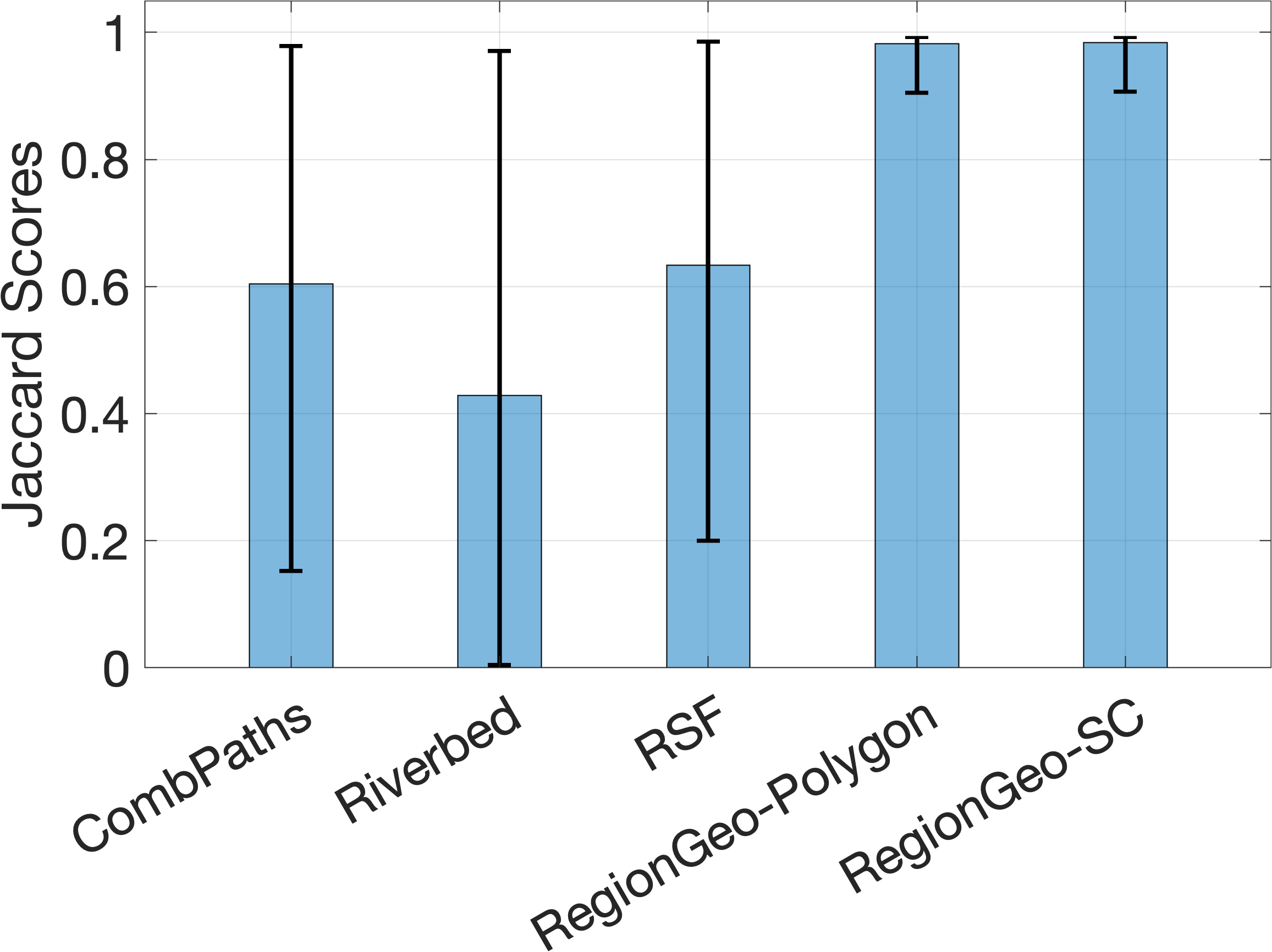
6.3.3 Computation Time
The computation complexity in our model mainly involve four parts: the construction of the initial contour, the estimation of the region-based energy gradients, the construction of tubular domains, and the extraction of geodesic paths. The last two parts can be efficiently solved by the fast marching methods whose computation complexity has been analyzed in Section 2.3. Here we report here the computation time for the image (with grid points) in row of Fig. 16. We apply the polygon construction method for the initial contour which cost seconds with three landmark points. The contour evolution process requires around seconds to stabilize. This test was conducted on an Intel Core i9 GHz architecture with GB RAM, using a C++ implementation for the FM-ASR method and a MATLAB implementation for the computation of regional energy gradients of the Bhattacharyya coefficient-based term.
7 Conclusion
In this paper, we propose a new region-based Randers geodesic model based on the eikonal PDE framework, which is an efficient solution to the active contour problem involving a regional appearance term. The core contributions of this paper lie at (i) the theoretical convergence analysis of the proposed geodesic model, (ii) the construction of Randers geodesic metrics, by which the region-based appearance term can be transformed to a weighted curve length in terms of a tubular domain, and (iii) a practical implementation of the introduced Randers geodesic model enhanced by various heuristics for practical interactive image segmentation, in conjunction with a collection of landmark points placed at the target boundary. The comparison results against state-of-the-art optimal paths-based segmentation models illustrate the advantages of taking the region-based appearance models for the computation of minimal geodesic paths and for image segmentation.
Future works will be devoted to (i) extending the proposed region-based Randers geodesic model to 3D volume segmentation in conjunction with the surface reconstruction method (Ardon and Cohen 2006), and (ii) integrating the proposed geodesic model with geometric shape priors for solving various medical image segmentation problems.
Acknowledgment
The authors would like to thank all the anonymous reviewers for their invaluable suggestions to improve this manuscript. This work is in part supported by the Shandong Provincial Natural Science Foundation (NO. ZR2022YQ64), a project in QLUT (NO. 2022PY11), the National Natural Science Foundation of China (NOs. 62171125, 62172243), the Intergovernmental Cooperation Project of the National Key Research and Development Program of China (NO. 2022YFE0116700), and by the French government under management of Agence Nationale de la Recherche as part of the “Investissements d’avenir” program, reference ANR-19-P3IA-0001 (PRAIRIE 3IA Institute).
Appendix A Proof of Theorem 3.2
This appendix is devoted to the proof of Theorem 3.2. We first estimate in Proposition 10 the curvature of a minimal path, which is bounded (but no necessarily continuous) under our assumptions. The Lagrangian formalism is used to describe the geometry, rather than the metric formalism (1), in order to benefit from the strict convexity property (92). In the application of this result, at the end of this section and following common practice, the Lagrangian is eventually defined as half the squared metric. We then show in Proposition 11 that a path with bounded curvature lying within a thin band can be parametrized as desired.
Proposition 10
Let be an open convex domain, equipped with a Lagrangian , with a continuous derivative w.r.t. the second variable, and such that:
| (89) | ||||
| (90) | ||||
| (91) | ||||
| (92) | ||||
| (93) |
for all , , , where are constants. Define
| (94) | ||||
| (95) |
where and . Then this minimum is attained, and any minimizer satisfies
| (96) | ||||
| (97) | ||||
| (98) | ||||
| (99) |
for all , where the constants depend on . In particular, the curvature satisfies .
Proof
We first observe that, for all and ,
| (100) |
using (i) the uniform convexity (92) with and noting that by Eq. 91, and (ii) Euler’s identity for -homogeneous functions. It follows that for any . This implies (96) using (i) by e.g. Jensen’s inequality for the left estimate, and (ii) choosing the straight line for the right estimate, which is a valid path since is convex.
From the compact embedding (Dacorogna 1989, Theorem 1.6 due to Sobolev and Rellich), and the weak compactness of the unit ball of (Banach-Alaoglu theorem), we obtain that there is a minimizing sequence for Eq. 95 which is converging, both weakly and uniformly, to a limit . Define
| (101) |
where denotes the Legendre-Fenchel dual of , referred to as the Hamiltonian, which is continuous. (Indeed, the inherits the Lipchitz-like regularity (89) w.r.t. , and by Eq. 92 it has a -Lipschitz gradient w.r.t. .) By construction , and by weak and uniform convergence for any continuous , hence and therefore minimizes (95).
We now fix a minimizer , and observe that by the -homogeneity property (93) it must be parametrized in such way that the Lagrangian is constant along the trajectory, establishing (97) for a.e. . Thus Eq. 98 follows, using Eqs. (96) and (100), with .
Let , and note that and on . Then
using successively (i) the optimality of , (ii) the definitions of and , and (iii) the Lipschitz-like property (89). Denoting and we obtain
using successively (i) the uniform convexity (92) of , and (ii) the fact that . Thus
using (i) the two previous estimates, and (ii) the Hölder semi-norm inequality on the domain , the estimates by Eq. (100, right), and by Eq. 90. It follows that with .
Denote by the averaging operator over the interval , and observe that hence the previous estimate amounts to . Therefore, for any ,
using (i) the previous estimate applied to , (ii) the Lipschitz bound (98, right) with . By (García-Cuerva and Gatto 2005, Theorem 2.3, using ), the mapping has Lipschitz regularity, with a Lipschitz constant equivalent to , which proves (99). The curvature bound follows from its definition (19), which concludes the proof. ∎
Proposition 11
Let and let whose absolute curvature is bounded by , with and . Denote and assume that that and . Then admits a reparametrization of the form , with where .
Proof
We may assume w.l.o.g. that is parametrized at unit Euclidean speed, thus , and in addition there exists such that for all . By assumption .
Now let . Assuming that and , we obtain
Note that , hence . It follows that , and by assumption . In general, distinguishing cases depending on the signs of and , we obtain . Observe that these two connected components of are disjoint, that is Lipschitz hence continuous, and that . Therefore for all , and the result follows. ∎
Conclusion of the proof of Theorem 3.2. We let , and note that is a local diffeomorphism. Defining , we obtain a Randers metric on , often referred to as the pull-back of the metric by , with Lipschitz coefficients (transformed as follows: and ).
Define the Lagrangian on . One easily checks that (89) to (93) hold on . In particular, the uniform convexity (92) follows from the fact that the ball associated to the Randers metric at a given point is an ellipsoid containing the origin in its iterior (but possibly not centered on the origin, contrary to the Riemannian case), hence is a uniformly convex set. In addition, paths minimizing the Finslerian length or the action (94) between two points are identical, up to a time reparametrization enforcing (97).
Denote by the endpoint in Theorem 3.2, and let . Any curve with can be expressed as a composition where is such that and . Furthermore by definition of the pullback metric.
Denote by a minimal geodesic path for the Lagrangian from to within . By Proposition 10, the curvature of is bounded by a constant, independent of the tube width . By Proposition 11, up to reducing , one has with . The curve is the solution to Eq. 22, and the proof is complete.
Appendix B Computation of Edge-based Features
Edge Saliency Features. Let be a vector-valued image in the RGB color space. The mollified Jacobian matrix of the image , with shape , is
where is a Gaussian kernel with standard deviation and (resp. ) denotes the first-order derivative of the kernel along the axis (resp. the axis ).
The edge saliency features can be described through a scalar-valued function which assigns to each point the Frobenius norm of the matrix
| (102) |
Edge Anisotropy Feature. As introduced in (Sochen et al 1998), the edge anisotropy feature at each point is carried out by a matrix defined as
| (103) |
where denotes the identity matrix of shape ( is the dimension of the image domain). For each point , the image gradient vector is derived as the eigenvector of which corresponds to its largest eigenvalue.
We finally discuss the special case of a gray level image . Then the function is obtained as
| (104) |
where stands for the standard Euclidean gradient of the Gaussian kernel .
At each point , the edge anisotropy feature matrix is expressed in terms of the vector field . Then the gradient vector field of a gray level image is taken as the eigenvector of corresponding to the largest eigenvalue. For the points such that , one has .
Appendix C RSF Geodesic Segmentation Model
The RSF geodesic model proposed by (Duits et al 2018) is a curvature-penalized model, that is defined over an orientation-lifted space. Let denote the angular space. A point consists of a position and of an angular coordinate . In this way, a smooth curve can be lifted to the space , i.e. , where is a parametric function such that for any and is the unit vector associated to the angle . The curve is referred to as the physical projection of .
The RSF model takes into account an orientation-lifted geodesic metric , which reads
where is a tangent vector to at point . In this case, the length of a smooth curve can be formulated as
| (105) |
where is a data-driven cost function. The value of is low if is close to an edge and the vector is tangent to that edge. As implemented in (Chen et al 2017), the computation of is carried out by the Canny-like steerable filter (Jacob and Unser 2004) for the following experiments.
RSF Segmentation Method. We leverage the RSF geodesic paths for interactive image segmentation, by connecting a set of landmark points with known order as input. This is implemented by exploiting a slight variant of the closed contour detection scheme introduced in (Chen et al 2017). Firstly, each landmark point is lifted to the orientation-lifted space such that corresponds to two points . The angle characterizes the orientation that an image edge should have at the point , which can be estimated by solving
At the initialization stage (i.e. ), we can get four RSF geodesic paths by choosing one point from as source point and choosing one point from as target point, respectively. Among them, we select the geodesic path with the smallest geodesic distance, whose source and target points are respectively denoted by and . This can be done by performing the Hamiltonian FMM (Mirebeau 2018) just once, as introduced in (Chen et al 2017). When , we can obtain two curvature-penalized geodesic paths joining the point to the orientation-lifted points and , respectively. From them, we again choose the minimal one in terms of geodesic distance associated to the RSF metric. In case , we iterate the similar step with until a geodesic path is tracked which takes the point as target point. In this way, we obtain orientation-lifted geodesic paths, whose physical projection curves form a closed contour passing through all the landmark points with .
References
- Abate and Tovena (2012) Abate M, Tovena F (2012) Curves and Surfaces. UNITEXT, Springer Science & Business Media, DOI 10.1007/978-88-470-1941-6“˙5
- Adams and Fournier (2003) Adams RA, Fournier JJ (2003) Sobolev spaces. Elsevier
- Alvarez et al (2018) Alvarez L, Cuenca C, Díaz JI, González E (2018) Level set regularization using geometric flows. SIAM J Imaging Sci 11(2):1493–1523
- Appia and Yezzi (2011) Appia V, Yezzi A (2011) Active geodesics: Region-based active contour segmentation with a global edge-based constraint. In: Proc. ICCV, IEEE, pp 1975–1980
- Appleton and Talbot (2005) Appleton B, Talbot H (2005) Globally optimal geodesic active contours. J Math Imaging Vis 23(1):67–86
- Arbelaez et al (2011) Arbelaez P, Maire M, Fowlkes C, Malik J (2011) Contour detection and hierarchical image segmentation. IEEE Trans Pattern Anal Mach Intell 33(5):898–916
- Ardon and Cohen (2006) Ardon R, Cohen LD (2006) Fast constrained surface extraction by minimal paths. Int J Comput Vis 69:127–136
- Bae and Tai (2011) Bae J Eand Yuan, Tai XC (2011) Global minimization for continuous multiphase partitioning problems using a dual approach. Int J Comput Vis 92(1):112–129
- Bao et al (2012) Bao D, Chern SS, Shen Z (2012) An introduction to Riemann-Finsler geometry, vol 200. Springer Science & Business Media
- Bardi and Capuzzo-Dolcetta (2008) Bardi M, Capuzzo-Dolcetta I (2008) Optimal Control and Viscosity Solutions of Hamilton-Jacobi-Bellman Equations. Birkhäuser 78:79
- Benmansour and Cohen (2009) Benmansour F, Cohen LD (2009) Fast object segmentation by growing minimal paths from a single point on 2D or 3D images. J Math Imaging Vis 33(2):209–221
- Bertelli et al (2008) Bertelli L, Sumengen B, Manjunath B, Gibou F (2008) A variational framework for multiregion pairwise-similarity-based image segmentation. IEEE Trans Pattern Anal Mach Intell 30(8):1400–1414
- Boggs and Tolle (1995) Boggs P, Tolle J (1995) Sequential quadratic programming. Acta Numerica 4:1–51
- Bougleux et al (2008) Bougleux S, Peyré G, Cohen LD (2008) Anisotropic geodesics for perceptual grouping and domain meshing. In: Proc. ECCV, pp 129–142
- Bourgain and Brezis (2003) Bourgain J, Brezis H (2003) On the equation and application to control of phases. Journal of the American Mathematical Society 16(2):393–426
- Boykov and Kolmogorov (2003) Boykov Y, Kolmogorov V (2003) Computing geodesics and minimal surfaces via graph cuts. In: Proc. ICCV, p 26
- Boykov and Kolmogorov (2004) Boykov Y, Kolmogorov V (2004) An experimental comparison of min-cut/max-flow algorithms for energy minimization in vision. IEEE Trans Pattern Anal Mach Intell 26(9):1124–1137
- Bresson and Chan (2008) Bresson X, Chan TF (2008) Non-local unsupervised variational image segmentation models. UCLA cam report 8:67
- Bresson et al (2006) Bresson X, Vandergheynst P, Thiran JP (2006) A variational model for object segmentation using boundary information and shape prior driven by the Mumford-Shah functional. Int J Comput Vis 68(2):145–162
- Bresson et al (2007) Bresson X, Esedoḡlu S, Vandergheynst P, Thiran J, Osher S (2007) Fast global minimization of the active contour/snake model. J Math Imaging Vis 28(2):151–167
- Brox and Cremers (2009) Brox T, Cremers D (2009) On local region models and a statistical interpretation of the piecewise smooth Mumford-Shah functional. Int J Comput Vis 84(2):184–193
- Brox and Weickert (2006) Brox T, Weickert J (2006) Level set segmentation with multiple regions. IEEE Trans Image Process 15(10):3213–3218
- Burago et al (2022) Burago D, Burago Y, Ivanov S (2022) A Course in Metric Geometry, Graduate Studies in Mathematics, vol 33. American Mathematical Society, DOI 10.1090/gsm/033/10
- Caselles et al (1997) Caselles V, Kimmel R, Sapiro G (1997) Geodesic active contours. Int J Comput Vis 22(1):61–79
- Chambolle et al (2012) Chambolle A, Cremers D, Pock T (2012) A convex approach to minimal partitions. SIAM J Imaging Sci 5(4):1113–1158
- Chan and Vese (2001) Chan TF, Vese LA (2001) Active contours without edges. IEEE Trans Image Process 10(2):266–277
- Chan et al (2000) Chan TF, Sandberg BY, Vese LA (2000) Active contours without edges for vector-valued images. J Vis Commun Image Represent 11(2):130–141
- Chan et al (2006) Chan TF, Esedoglu S, Nikolova M (2006) Algorithms for finding global minimizers of image segmentation and denoising models. SIAM J Appl Math 66(5):1632–1648
- Chen and Cohen (2017) Chen D, Cohen LD (2017) Anisotropic edge-based balloon Eikonal active contours. In: Proc. GSI, pp 782–790
- Chen and Cohen (2018) Chen D, Cohen LD (2018) Fast asymmetric fronts propagation for image segmentation. J Math Imaging Vis 60(6):766–783
- Chen et al (2016) Chen D, Mirebeau JM, Cohen LD (2016) Finsler geodesics evolution model for region based active contours. In: Proc. BMVC, pp 22.1–22.12
- Chen et al (2017) Chen D, Mirebeau JM, Cohen LD (2017) Global minimum for a Finsler elastica minimal path approach. Int J Comput Vis 122(3):458–483
- Chen et al (2021a) Chen D, Cohen LD, Mirebeau JM, Tai XC (2021a) An elastica geodesic approach with convexity shape prior. In: Proc. ICCV, pp 6900–6909
- Chen et al (2021b) Chen D, Spencer J, Mirebeau JM, Chen K, Shu M, Cohen LD (2021b) A generalized asymmetric dual-front model for active contours and image segmentation. IEEE Trans Image Process 30:5056–5071
- Chen et al (2021c) Chen D, Zhu J, Zhang X, Shu M, Cohen LD (2021c) Geodesic paths for image segmentation with implicit region-based homogeneity enhancement. IEEE Trans Image Process 30:5138–5153
- Chen et al (2022) Chen D, Mirebeau JM, Shu M, Tai X, Cohen LD (2022) Geodesic models with convexity shape prior. IEEE Trans Pattern Anal Mach Intell DOI 10.1109/TPAMI.2022.3225192
- Choi et al (1997) Choi HI, Choi SW, Moon HP (1997) Mathematical theory of medial axis transform. Pacific Journal of Mathematics 181(1):57–88
- Cohen (1991) Cohen LD (1991) On active contour models and balloons. CVGIP: Image Understand 53(2):211–218
- Cohen (1997) Cohen LD (1997) Avoiding local minima for deformable curves in image analysis. Curves and Surfaces with Applications in CAGD pp 77–84
- Cohen (2001) Cohen LD (2001) Multiple contour finding and perceptual grouping using minimal paths. J Math Imaging Vis 14(3):225–236
- Cohen and Cohen (1993) Cohen LD, Cohen I (1993) Finite-element methods for active contour models and balloons for 2-D and 3-D images. IEEE Trans Pattern Anal Mach Intell 15(11):1131–1147
- Cohen and Kimmel (1997) Cohen LD, Kimmel R (1997) Global minimum for active contour models: A minimal path approach. Int J Comput Vis 24(1):57–78
- Cremers et al (2002) Cremers D, Tischhäuser F, Weickert J, Schnörr C (2002) Diffusion snakes: Introducing statistical shape knowledge into the Mumford-Shah functional. Int J Comput Vis 50(3):295–313
- Cremers et al (2007) Cremers D, Rousson M, Deriche R (2007) A review of statistical approaches to level set segmentation: integrating color, texture, motion and shape. Int J Comput Vis 72(2):195–215
- Dacorogna (1989) Dacorogna B (1989) Direct Methods in the Calculus of Variations, Applied Mathematical Sciences, vol 78. Springer Science & Business Media, DOI 10.1007/978-3-642-51440-1
- Deschamps and Cohen (2001) Deschamps T, Cohen LD (2001) Fast extraction of minimal paths in 3D images and applications to virtual endoscopy. Med Image Anal 5(4):281–299
- Desquesnes et al (2013) Desquesnes X, Elmoataz A, Lézoray O (2013) Eikonal equation adaptation on weighted graphs: fast geometric diffusion process for local and non-local image and data processing. J Math Imag Vis 46:238–257
- Dijkstra (1959) Dijkstra EW (1959) A note on two problems in connexion with graphs. Numer Math 1(1):269–271
- Doğan et al (2008) Doğan G, Morin P, Nochetto RH (2008) A variational shape optimization approach for image segmentation with a Mumford–Shah functional. SIAM J Imag Sci 30(6):3028–3049
- Duan et al (2015) Duan Y, Chang H, Huang W, Zhou J, Lu Z, Wu C (2015) The {} regularized Mumford--Shah model for bias correction and segmentation of medical images. IEEE Trans Image Process 24(11):3927--3938
- Dubrovina-Karni et al (2015) Dubrovina-Karni A, Rosman G, Kimmel R (2015) Multi-region active contours with a single level set function. IEEE Trans Pattern Anal Mach Intell 37(8):1585–1601
- Duits et al (2018) Duits R, Meesters SP, Mirebeau JM, Portegies JM (2018) Optimal paths for variants of the 2D and 3D Reeds–Shepp car with applications in image analysis. J Math Imag Vis 60(6):816–848
- Fabbri et al (2008) Fabbri R, Costa L, Torelli J, Bruno O (2008) 2d euclidean distance transform algorithms: A comparative survey. ACM Computing Surveys (CSUR) 40(1):1–44
- Falcão et al (2000) Falcão AX, Udupa JK, Miyazawa FK (2000) An ultra-fast user-steered image segmentation paradigm: live wire on the fly. IEEE Trans Med Imaging 19(1):55–62
- Falcao et al (2004) Falcao AX, Stolfi J, de Alencar Lotufo R (2004) The image foresting transform: Theory, algorithms, and applications. IEEE Trans Pattern Anal Mach Intell 26(1):19–29
- Friedlander et al (1998) Friedlander FG, Joshi MS, Joshi M, Joshi MC (1998) Introduction to the Theory of Distributions. Cambridge University Press
- García-Cuerva and Gatto (2005) García-Cuerva J, Gatto AE (2005) Lipschitz spaces and Calderón-Zygmund operators associated to non-doubling measures. Publicacions matematiques pp 285–296
- Goldenberg et al (2001) Goldenberg R, Kimmel R, Rivlin E, Rudzsky M (2001) Fast geodesic active contours. IEEE Trans Image Process 10(10):1467–1475
- Grady and Alvino (2009) Grady L, Alvino CV (2009) The piecewise smooth Mumford–Shah functional on an arbitrary graph. IEEE Trans Image Process 18(11):2547–2561
- Houhou et al (2009) Houhou N, Thiran JP, Bresson X (2009) Fast texture segmentation based on semi-local region descriptor and active contour. Numerical Mathematics: Theory, Methods and Applications 2:445–468
- Jacob and Unser (2004) Jacob M, Unser M (2004) Design of steerable filters for feature detection using canny-like criteria. IEEE Trans Pattern Anal Mach Intell 26(8):1007–1019
- Jalba et al (2004) Jalba AC, Wilkinson MH, Roerdink JB (2004) CPM: A deformable model for shape recovery and segmentation based on charged particles. IEEE Trans Pattern Anal Mach Intell 26(10):1320–1335
- Jung (2017) Jung M (2017) Piecewise-smooth image segmentation models with data-fidelity terms. J Sci Comput 70(3):1229–1261
- Jung et al (2012) Jung M, Peyré G, Cohen LD (2012) Nonlocal active contours. SIAM J Imaging Sci 5(3):1022–1054
- Kass et al (1988) Kass M, Witkin A, Terzopoulos D (1988) Snakes: Active contour models. Int J Comput Vis 1(4):321–331
- Kimmel (2003) Kimmel R (2003) Fast edge integration. In: Geometric Level Set Methods in Imaging, Vision, and Graphics, Springer, pp 59–77
- Kimmel and Bruckstein (2003) Kimmel R, Bruckstein AM (2003) Regularized laplacian zero crossings as optimal edge integrators. Int J Comput Vis 53(3):225–243
- Li and Acton (2007) Li B, Acton ST (2007) Active contour external force using vector field convolution for image segmentation. IEEE Trans Image Process 16(8):2096–2106
- Li et al (2008) Li C, Kao C, Gore JC, Ding Z (2008) Minimization of region-scalable fitting energy for image segmentation. IEEE Trans Image Process 17(10):1940–1949
- Li et al (2010) Li F, Ng MK, Li C (2010) Variational fuzzy Mumford–Shah model for image segmentation. SIAM Journal on Applied Mathematics 70(7):2750–2770
- Lu and Shiou (2002) Lu TT, Shiou SH (2002) Inverses of block matrices. Computers & Mathematics with Applications 43(1-2):119–129
- Luo et al (2022) Luo S, Tai XC, Glowinski R (2022) Convex object(s) characterization and segmentation using level set function. J Math Imag Vis pp 1–21
- Ma et al (2021) Ma J, Wang D, Wang XP, Yang X (2021) A fast algorithm for geodesic active contours with applications to medical image segmentation. SIAM J Imag Sci
- Melonakos et al (2008) Melonakos J, Pichon E, Angenent S, Tannenbaum A (2008) Finsler active contours. IEEE Trans Pattern Anal Mach Intell 30(3):412–423
- Michailovich et al (2007) Michailovich O, Rathi Y, Tannenbaum A (2007) Image segmentation using active contours driven by the Bhattacharyya gradient flow. IEEE Trans Image Process 16(11):2787–2801
- Mille et al (2015) Mille J, Bougleux S, Cohen LD (2015) Combination of piecewise-geodesic paths for interactive segmentation. Int J Comput Vis 112(1):1–22
- Miranda et al (2012) Miranda PA, Falcao AX, Spina TV (2012) Riverbed: A novel user-steered image segmentation method based on optimum boundary tracking. IEEE Trans Image Process 21(6):3042–3052
- Mirebeau (2014a) Mirebeau JM (2014a) Anisotropic fast-marching on cartesian grids using lattice basis reduction. SIAM J Numer Anal 52(4):1573–1599
- Mirebeau (2014b) Mirebeau JM (2014b) Efficient fast marching with Finsler metrics. Numer Math 126(3):515–557
- Mirebeau (2018) Mirebeau JM (2018) Fast-marching methods for curvature penalized shortest paths. J Math Imag Vis 60(6):784–815
- Mirebeau (2019) Mirebeau JM (2019) Riemannian fast-marching on Cartesian grids, using Voronoi’s first reduction of quadraticforms. SIAM J Numer Anal 57(6):2608–2655
- Mirebeau and Desquilbet (2019) Mirebeau JM, Desquilbet F (2019) Worst case and average case cardinality of strictly acute stencils for two dimensional anisotropic fast marching. In: Constructive Theory of Functions
- Mishra et al (2011) Mishra AK, Fieguth PW, Clausi DA (2011) Decoupled active contour (DAC) for boundary detection. IEEE Trans Pattern Anal Mach Intell 33(2):310–324
- Morel and Solimini (2012) Morel JM, Solimini S (2012) Variational methods in image segmentation: with seven image processing experiments, vol 14. Springer Science & Business Media
- Mumford and Shah (1989) Mumford D, Shah J (1989) Optimal approximations by piecewise smooth functions and associated variational problems. Commun Pure Appl Math 42(5):577–685
- Ni et al (2009) Ni K, Bresson X, Chan T, Esedoglu S (2009) Local histogram based segmentation using the Wasserstein distance. Int J Comput Vis 84(1):97–111
- Osher and Sethian (1988) Osher S, Sethian JA (1988) Fronts propagating with curvature-dependent speed: algorithms based on Hamilton-Jacobi formulations. J Comput Phys 79(1):12–49
- Paragios and Deriche (2002) Paragios N, Deriche R (2002) Geodesic active regions: A new framework to deal with frame partition problems in computer vision. J Vis Commun Image Represent 13(1):249–268
- Peyré et al (2010) Peyré G, Péchaud M, Keriven R, Cohen LD (2010) Geodesic methods in computer vision and graphics. Foundations and Trends® in Computer Graphics and Vision 5(3–4):197–397
- Prevost et al (2014) Prevost R, Cuingnet R, Mory LD Band Cohen, Ardon R (2014) Tagged template deformation. In: Proc. MICCAI, Springer, pp 674–681
- Randers (1941) Randers G (1941) On an asymmetrical metric in the four-space of general relativity. Phys Rev 59(2):195
- Rother et al (2004) Rother C, Kolmogorov V, Blake A (2004) Grabcut: Interactive foreground extraction using iterated graph cuts. ACM Trans Graph 23(3):309–314
- Sethian (1999) Sethian JA (1999) Fast marching methods. SIAM Review 41(2):199–235
- Sethian and Vladimirsky (2003) Sethian JA, Vladimirsky A (2003) Ordered upwind methods for static Hamilton–Jacobi equations: Theory and algorithms. SIAM J Numer Anal 41(1):325–363
- Shi and Li (2021) Shi X, Li C (2021) Convexity preserving level set for left ventricle segmentation. Magn Reson Imaging 78:109–118
- Siu et al (2020) Siu CY, Chan HL, Ming Lui RL (2020) Image segmentation with partial convexity shape prior using discrete conformality structures. SIAM J Imaging Sci 13(4):2105–2139
- Sochen et al (1998) Sochen N, Kimmel R, Malladi R (1998) A general framework for low level vision. IEEE Trans Image Process 7(3):310–318
- Sokolowski et al (1992) Sokolowski J, Zolésio JP, Sokolowski J, Zolesio JP (1992) Introduction to shape optimization. Springer
- Sumengen and Manjunath (2006) Sumengen B, Manjunath B (2006) Graph partitioning active contours (GPAC) for image segmentation. IEEE Trans Pattern Anal Mach Intell 28(4):509–521
- Sundaramoorthi et al (2007) Sundaramoorthi G, Yezzi A, Mennucci AC (2007) Sobolev active contours. Int J Comput Vis 73(3):345–366
- Sundaramoorthi et al (2009) Sundaramoorthi G, Yezzi A, Mennucci AC, Sapiro G (2009) New possibilities with Sobolev active contours. Int J Comput Vis 84(2):113–129
- Thäle (2008) Thäle C (2008) 50 years sets with positive reach–a survey. Surveys in Mathematics and its Applications 3:123–165
- Tsai et al (2001) Tsai A, Yezzi A, Willsky AS (2001) Curve evolution implementation of the Mumford-Shah functional for image segmentation, denoising, interpolation, and magnification. IEEE Trans Image Process 10(8):1169–1186
- Tsitsiklis (1995) Tsitsiklis JN (1995) Efficient algorithms for globally optimal trajectories. IEEE Trans Automat Contr 40(9):1528–1538
- Vese and Chan (2002) Vese LA, Chan TF (2002) A multiphase level set framework for image segmentation using the Mumford and Shah model. Int J Comput Vis 50(3):271–293
- Windheuser et al (2009) Windheuser T, Schoenemann T, Cremers D (2009) Beyond connecting the dots: A polynomial-time algorithm for segmentation and boundary estimation with imprecise user input. In: Proc. ICCV, IEEE, pp 717–722
- Xie and Mirmehdi (2008) Xie X, Mirmehdi M (2008) MAC: Magnetostatic active contour model. IEEE Trans Pattern Anal Mach Intell 30(4):632–646
- Xu and Prince (1998) Xu C, Prince JL (1998) Snakes, shapes, and gradient vector flow. IEEE Trans Image Process 7(3):359–369
- Yang and Sundaramoorthi (2015) Yang Y, Sundaramoorthi G (2015) Shape tracking with occlusions via coarse-to-fine region-based sobolev descent. IEEE Trans Pattern Anal Mach Intell 37(5):1053–1066, DOI 10.1109/TPAMI.2014.2360380
- Yezzi et al (1997) Yezzi A, Kichenassamy S, Kumar A, Olver P, Tannenbaum A (1997) A geometric snake model for segmentation of medical imagery. IEEE Trans Med Imaging 16(2):199–209
- Younes (2019) Younes L (2019) Shapes and Diffeomorphisms, Applied Mathematical Sciences, vol 171. Springer, DOI 10.1007/978-3-662-58496-5“˙6
- Yuan et al (2014) Yuan J, Bae E, Tai XC, Boykov Y (2014) A spatially continuous max-flow and min-cut framework for binary labeling problems. Numer Math 126:559–587
- Zach et al (2009) Zach C, Shan L, Niethammer M (2009) Globally optimal Finsler active contours. In: Proc. Joint Pattern Recognition Symposium, Springer, pp 552–561
- Zhang and Lui (2021) Zhang D, Lui LM (2021) Topology-preserving 3D image segmentation based on hyperelastic regularization. J Sci Comput 87(3):74
- Zhang et al (2021) Zhang D, Tai XC, Lui LM (2021) Topology- and convexity-preserving image segmentation based on image registration. Appl Math Model 100:218–239
- Zhang et al (2019) Zhang W, Wang X, You W, Chen J, Dai P, Zhang P (2019) RESLS: Region and edge synergetic level set framework for image segmentation. IEEE Trans Image Process 29:57–71
- Zhu and Yuille (1996) Zhu S, Yuille A (1996) Region competition: Unifying snakes, region growing, and Bayes/MDL for multiband image segmentation. IEEE Trans Pattern Anal Mach Intell 18(9):884–900