New CTEQ global analysis of quantum chromodynamics with high-precision data from the LHCPreprint: MSUHEP-19-025, PITT-PACC-1911, SMU-HEP-19-03
Abstract
We present the new parton distribution functions (PDFs) from the CTEQ-TEA collaboration, obtained using a wide variety of high-precision Large Hadron Collider (LHC) data, in addition to the combined HERA I+II deep-inelastic scattering data set, along with the data sets present in the CT14 global QCD analysis. New LHC measurements in single-inclusive jet production with the full rapidity coverage, as well as production of Drell-Yan pairs, top-quark pairs, and high- bosons, are included to achieve the greatest sensitivity to the PDFs. The parton distributions are determined at NLO and NNLO, with each of these PDFs accompanied by error sets determined using the Hessian method. Fast PDF survey techniques, based on the Hessian representation and the Lagrange Multiplier method, are used to quantify the preference of each data set to quantities such as , and the gluon and strange quark distributions. We designate the main resulting PDF set as CT18. The ATLAS 7 TeV precision data are not included in CT18, due to their tension with other data sets in the global fit. Alternate PDF sets are generated including the ATLAS precision 7 TeV data (CT18A), a new scale choice for low- DIS data (CT18X), or all of the above with a slightly higher choice for the charm mass (CT18Z). Theoretical calculations of standard candle cross sections at the LHC (such as the fusion Higgs boson cross section) are presented.
pacs
12.38.-t,12.38.Bx,12.38.AwI Introduction
With an accumulated data sample of over 140 fb-1 at the 13 TeV run for both ATLAS and CMS collaborations, the Large Hadron Collider (LHC) has entered an era of precision physics. The experimental precision has been matched by improvements to the theoretical predictions, with a number of collider processes now available at the next-to-next-to-leading order (NNLO) in the QCD coupling strength. Such precision is necessary for rigorous tests of the Standard Model (SM) and in searches for signs of physics beyond the Standard Model (BSM), as there have been no ‘smoking-gun’ signs of BSM physics to date. Precise predictions in QCD theory require correspondingly precise parton distribution functions (PDFs) Dulat et al. 2016; Harland-Lang et al. 2015a; Ball et al. 2017; Alekhin et al. 2017; Accardi et al. 2016a; Harland-Lang et al. 2019; Bertone et al. 2018; Manohar et al. 2017, which in turn warrant advances in interpreting LHC experiments to extract important information about the SM, and possibly, BSM physics.
To this end, we present a new family of CTEQ-TEA parton distribution functions, designated as CT18. These PDFs are produced at both next-to-leading order (NLO) and NNLO in the QCD coupling constant, . The CT18 PDFs update those of the CT14 family presented in Ref. Dulat et al. 2016. In the new analysis, we include a variety of new LHC data, at the center-of-mass energies of 7 and 8 TeV, on production of single-inclusive jets, bosons, and top-antitop quark pairs, obtained by the ATLAS, CMS and LHCb collaborations. At the same time, the update retains crucial “legacy” data from the previous CT global QCD analyses, such as the HERA I+II combined data on deep-inelastic scattering (DIS) and measurements in fixed-target experiments and at the Fermilab Tevatron collider. Measurements of processes in similar kinematic regions, by both ATLAS and CMS, allow crucial cross-checks of the data. Measurements by LHCb often allow extrapolations into new kinematic regions not covered by the other experiments. Some processes, such as production, allow for the measurement of multiple observables that provide similar information for the determination of PDFs. In addition to the PDFs themselves, we also present relevant PDF luminosities, and predictions with uncertainties for standard candle cross sections at the LHC.
The goal of the CT18 analysis is to include as wide a kinematic range for each measurement as possible, while still achieving reasonable agreement between data and theory. For the ATLAS 7 TeV jet data Aad et al. 2015, for example, all rapidity intervals cannot be simultaneously used without the introduction of systematic error decorrelations provided by the ATLAS collaboration Aaboud et al. 2017a. Even with that decorrelation, the resultant for the new jet experiments is not optimal, resulting in less effective PDF constraints. Inclusive cross section measurements for jet production have been carried out for two different jet-radius values, , by both ATLAS and CMS. For both experiments, we have chosen the data with the larger -value, for which the NNLO (fixed order) prediction should have a higher accuracy. We evaluate the jet cross section predictions using a QCD scale of inclusive jet transverse momentum , consistent with past usage at NLO. The result is largely consistent with similar evaluations using Currie et al. 2017a; Currie et al. 2017b; Currie et al. 2018.
Theoretical predictions for comparison to the data used in the global fit have been carried out at NNLO, either indirectly through the use of fast interpolation tables such as fastNLO Britzger et al. 2012; Wobisch et al. 2011 and ApplGrid Carli et al. 2010, together with NNLO/NLO -factors, or directly (for top-quark related observables) through the use of fastNNLO grids Czakon et al. 2017a; fas.
In an ideal world all such data sets would perfectly be compatible with each other, but differences are observed that do result in some tension between data sets and pulls in opposite directions. One of the crucial aspects of carrying out a global PDF analysis is dealing with data sets that add some tension to the fits, while preserving the ability of the combined data set to improve on the existing constraints on the PDFs. In some cases, a data set may be in such tension as to require its removal from the global analysis, or its inclusion only in a separate iteration of the new PDF set.
In this paper, we will describe how the high-precision ATLAS 7 TeV rapidity distributions, which, as we find, favor an increase of the strange quark distribution at low , require such special treatment. In particular, while other PDF-analysis groups (e.g., MMHT, see Ref. Thorne et al. 2019) have noted that these ATLAS data can be fitted with that is comparable to the CT18 one, we find that such reflects systematic tensions with many of the other data in our global analysis. Furthermore, the standard Hessian profiling technique used by the experimental collaborations significantly underestimates the minimal that can be reached for the ATLAS 7 TeV data when they are included in the CT18 fit. We therefore treat these measurements separately in an alternative fit, CT18A, introduced in Sec. II.3. In another variant, CT18X, a special scale is used for the calculation of low- DIS cross sections; the scale mimics the impact of low- resummation. Both modifications cause an increase in the low- quark and gluon distributions. Finally, these two variants of the CT18 fit are amalgamated into a combined alternative fit, CT18Z. Since the CT18Z PDFs are most dissimilar from the CT18 ones, we show numerous results based on the CT18 and CT18Z PDFs throughout the article, while deferring the comparisons to CT18A and X to Appendix A, where additional in-depth comparisons to CT18Z are also provided. A recommendation on selecting one of the four PDF ensembles depending on the user’s needs is given at the beginning of Sec. VII.
Our current global analyses are carried out in four stages. First, PDFSense Wang et al. 2018; Hobbs et al. 2019, a program for a rapid survey of QCD data using the Hessian approach Pumplin et al. 2001; Pumplin et al. 2002, is used to select the data sets that are expected to have the greatest impact on the global PDF sets. This selection takes into account the sensitivity of the data to specific PDFs in a given range, which reflects both the correlation of these data with a given PDF, as well the size of the data set and magnitudes of its statistical and correlated systematic errors. For example, both the collider inclusive jet data and the top-quark data have a strong correlation with the high- gluon, but the inclusive jet data has a larger sensitivity due to a much larger number of data points. Next, ePump Schmidt et al. 2018; Hou et al. 2019 is used to quickly examine the quantitative impact of each selected data set, within the Hessian approximation. Third, the full global PDF fit is carried out using all such data sets. Recent enhancements to the CT global analysis code have greatly improved the speed of the calculations. Lastly, the impact of key data sets on certain PDFs at specific kinematic points of interest, as well as on the value of , is assessed using the Lagrange Multiplier (LM) method Stump et al. 2001. In order to minimize any parametrization bias, we have tested different parametrizations for CT18: e.g., using a more flexible parametrization for the strange quark PDF. In some kinematic regions, there are fewer constraints from the data on certain PDFs. In particular, LM constraints have been applied to limit the strangeness PDF at to physically reasonable values, as summarized in App. C.
Our paper is organized as follows. Section II begins with an executive summary of the key stages and results of the CT18 global analysis. It continues with an overview of the chosen experimental data and alternative fits (CT18Z, CT18A, and CT18X) in the CT18 release. This section concisely summarizes the key results that are of interest to most readers. The subsequent sections and appendices elaborate on specific aspects and outcomes.
In Sec. III we detail theoretical/computational updates to the CT fitting methodology and details for specific process-dependent calculations. Sec. IV presents the main results obtained in CT18 — the fitted PDFs as functions of and , determinations of QCD parameters (, ), calculated parton luminosities, and various PDF moments and sum rules. These comparisons be of interest to a broad group of researchers who will use the PDFs for theoretical predictions at LHC experiments.
Sec. V describes the ability of CT18 to provide a successful theoretical description of the fitted data. In addition to characterizing the fit of individual data sets, in Sec. VI we also compute the various standard candle quantities of relevance to LHC phenomenology, for instance, Higgs boson production cross sections at and TeV, and various correlations among electroweak boson and top-quark pair production cross sections. In Sec. VII, we discuss the broader implications of this work and highlight our main conclusions.
Several appendices present a number of important supporting details. In Appendix A, we review the CT18Z and other alternative fits, including descriptions of various data sets admitted into these separate analyses. A number of more formal details related to our likelihood functions and relations among covariance matrices are summarized in Appendix B. Appendix C presents the analytical fitting form adopted in CT18 and best-fit values of the PDF parameters. Appendix D presents a number of technical advances in the CT fitting framework, including code parallelization, while Appendix E enumerates the decorrelation models utilized in fitting the newly included inclusive jet data from the LHC. Lastly, in Appendix F, we present the results of a short study based on Hessian profiling methods to assess the impact of the 7 TeV production data taken by ATLAS.
II Overview of the CT18 global QCD analysis
II.1 Executive Summary
II.1.1 Input experimental data and final PDF ensembles
The CT18 analysis updates the widely used CT14 PDF sets Dulat et al. 2016 by applying NNLO and NLO global fits to an expanded set of experimental measurements that include high-statistics data from the collider HERA and the LHC. The CT18 experimental data set includes high-statistics measurements from ATLAS, CMS, and LHCb on production of inclusive jets, bosons, and top-quark pairs, while it retains the crucial legacy data, such as the HERA Run I and Run II combined data and measurements from the Tevatron. By 2018, the LHC collaborations published about three dozen experimental data sets that can potentially constrain the CT PDFs. We selected the most promising experiments available by mid-2018 using the methods reviewed in Secs. II.1.3 and II.1.4. We then extensively examined the impacts of the data sets within the full fitting framework. Sec. II.2 contains an overview of these experiments. The kinematic distribution of the data points included in CT18 is shown in Fig. 1 as a function of the typical parton momentum fraction, , and QCD factorization scale, denoted here as .11 1 The typical momentum fractions and factorization scales are estimated as in Ref. Wang et al. 2018. As has been true for global PDF fits for some time, the data included cover a large kinematic range, both in and .
In light of the unprecedented precision reached in some measurements, the latest LHC data must be analyzed using NNLO theoretical predictions in perturbative QCD. The fitted PDFs we obtain in this analysis are plotted in Fig. 2, which displays in the upper panels the CT18 PDFs at two widely-separated scales, and GeV (on the left and right, respectively). In the lower panels, we show the corresponding PDFs found in our amalgamated alternative analysis, CT18Z.
The final CT18(Z) data ensemble contains a total of 3681 (3493) data points and results in at NNLO. The PDF uncertainties are constructed at the 90% probability level based on two tiers of criteria as in the CT14 global analysis Dulat et al. 2016. These PDFs are obtained by assuming a world-average QCD coupling constant, Tanabashi et al. 2018. The combined PDF+ uncertainty can be computed using the special series of the PDFs for each family by adding the PDF and uncertainties in quadrature, as explained in Ref. Lai et al. 2010a.
Among the four ensembles (CT18, A, X, and Z) of PDFs, the CT18 and CT18Z ensembles are the most dissimilar in terms of the shapes of PDFs, notably in the dependence of the fitted gluon and strangeness distributions, and , as well as in some PDF uncertainties. For CT18, we obtain modest improvements in the precision for the gluon density , as compared to CT14, following the inclusion of the LHC Run-1 data discussed below. For CT18Z, however, we obtain a somewhat enlarged uncertainty for the gluon and perturbatively-generated charm PDFs, especially at the lowest values of , due to the modified treatment of the DIS data described in Sec. II.3 and App. A. These final PDFs depend on numerous systematic factors in the experimental data. Scrupulous examination of the systematic effects was essential for trustworthy estimates of PDF uncertainties, and the scope of numerical computations also needed to be expanded.
II.1.2 Combined HERA I+II DIS data and the -dependent factorization scale
Even in the LHC era, DIS data from the collider HERA provide the dominant constraints on the CT18 PDFs. This dominance is revealed by independently applying the ePump, PDFSense, and Lagrange Multiplier methods. CT18 implements the final (“combined”) data set from DIS at HERA Run-I and Run-II Abramowicz et al. 2015 that supersedes the HERA Run-I only data set Aaron et al. 2010 used in CT14 Dulat et al. 2016. A transitional PDF set, CT14, was released based on fitting the final HERA data Hou et al. 2017a. We found fair overall agreement of the HERA I+II data with both CT14 and CT14 PDFs, and that both PDF ensembles describe equally well the non-HERA data included in our global analysis. At the same time, we observed some disagreement (“statistical tension”) between the and DIS cross sections of the HERA I+II data set. We determined that, at the moment, no plausible explanation could be provided to describe the full pattern of these tensions, as they are distributed across the whole accessible range of Bjorken and lepton-proton momentum transfer at HERA. Extending these studies using the CT18 fit, we have investigated the impact of the choice of QCD scales on inclusive DIS data in the small- region, as will be explained later in Sec. II.3.
We find that the quality of fit to HERA data is improved by about 50 units by evaluating the NNLO theoretical cross sections in DIS with a special factorization scale, , that depends on Bjorken (not the momentum fraction ) and is introduced in Section II.3. Fig. 3 (left) shows the changes in the candidate CT18 PDFs obtained by fitting the DIS data sets with the factorization scale , as compared to the CT18 PDFs with the nominal scale . With the scale , we observe reduced and (anti-)quark PDFs and increased gluon and strangeness PDFs at , as compared to the nominal CT18 fit, with some compensating changes occurring in the same PDFs in the unconstrained region in order to satisfy the valence and momentum sum rules.
The right panel of Fig. 3 shows the values ( divided by the number, , of experimental data points) for four HERA data sets (inclusive neutral and charged current DIS Abramowicz et al. 2015, reduced charm, bottom production cross sections, and H1 longitudinal function Aaron et al. 2011) in the fits as a function of the statistical weight of the HERA I+II inclusive DIS data set Abramowicz et al. 2015. The default CT18Z fit corresponds to ; with , the CT18Z fit increasingly behaves as a HERA-only fit. We see that, with the scale and , for the inclusive DIS data set improves almost to the levels observed in the “resummed” HERA-only fits without intrinsic charm Ball et al. 2018; Abdolmaleki et al. 2018. The quality of the fit to the charm semi-inclusive DIS (SIDIS) cross section and H1 also improves. 22 2 The use of the separate H1 data as well as the HERA-II combined data introduces some double counting. However, we have checked that this choice does not appreciably change the PDFs, while it does provide a useful indicator of the goodness of fit in the small- region. In particular, it is telling that the total value of H1 data (ID=169) becomes smaller, not larger, in the CT18X and CT18Z fits, as compared to CT18.
The new combined charm and bottom production measurements from the H1 and ZEUS collaborations published in Ref. Abramowicz et al. 2018 (2018) have been investigated and in their current version, when these measurements replace the previous ones in the CT18 global analysis, they cannot be fitted with a reasonable . Moreover, a mild tension is observed between these new combined data and several CT18 data sets such as the LHCb 7 and 8 TeV production data, -rapidity data at CDF run II, CMS 8 TeV single inclusive jet production, and double differential and cross section. Therefore, we decided not to include these data in the CT18 global analysis as they require a dedicated investigation. In the H1+ZEUS analysis of Ref. Abramowicz et al. 2018, the for these measurements is also found not to be optimal. This is ascribed to a difference in the slope between data and theory in the intermediate/small region. In our attempt to fit the new combined charm and bottom production measurements, we have noticed a preference for a harder gluon at intermediate/small . We are currently investigating these data separately and, in particular, we are exploring the impact of the new correlated systematic uncertainties as they increased from 42 in the old version of the data, to 167 in the new version. The results of this new study are going to be published in a separate forthcoming paper.
II.1.3 Selection of new LHC experiments
When selecting the most promising LHC experiments for the CT18 fit, we had to address a recurrent challenge — the presence of statistical tensions among various (sub)sets of the latest experimental data from HERA, LHC, and the Tevatron. The quickly improving precision of the collider data reveals previously irrelevant anomalies either in the experiment or theory. These anomalies are revealed by applying strong goodness-of-fit tests Kovařík et al. 2019. Figure 4 illustrates the degree of tensions using a representation based on the effective Gaussian variables Lai et al. 2010b constructed from the values and numbers of data points for individual data sets . In an ideal fit in which the differences between theory and data are consistent with Gaussian random fluctuations, the probability distribution for must be approximately a standard normal distribution (with a unit half-width). In the global fits by CTEQ-TEA and external groups, we rather observe wider distributions as in Fig. 4, with some of the more comprehensive and precise data sets (notably, HERA I+II inclusive DIS Abramowicz et al. 2015 and ATLAS 7 TeV production Aaboud et al. 2017b) having values as high as five units or more. The question, then, is how to select clean and accurate experiments for the global analysis from an ever-growing list of measurements, while maximally preserving the consistency of the selected experiments. For example, there are many LHC data sets Rojo et al. 2015 that are potentially sensitive to the PDFs, including novel measurements involving the production of high- bosons, pairs, isolated photon, and small- heavy flavor (charm or bottom) quarks. Including all such candidate experiments into the full global fit is impractical: CPU costs grow quickly with the number of experimental data sets at NNLO. Poorly fitted experiments would increase, not decrease, the final PDF uncertainty. The generation of one error PDF set took several days of CPU time in the CT14 fit to 33 experiments in single-thread mode. Adding 20-30 additional experiments with this setup was thus impossible. The CTEQ-TEA group resolved these challenges through a multi-pronged effort that allowed us to include eleven new LHC data sets at 7 and 8 TeV on , , jet, and production.
II.1.4 Advances in fitting methodology
To identify the eligible experimental data sets for the global fit, we developed two programs for fast preliminary analysis. The PDFSense program Wang et al. 2018 was developed at Southern Methodist University (SMU) to predict quantitatively, and before doing the fit, which data sets will have an impact on the global PDF fit. The ePump program Schmidt et al. 2018 developed at Michigan State University (MSU) applies Hessian profiling to quickly estimate the impact of data on the PDFs prior to the global fit. These programs provide helpful guidelines for the selection of the most valuable experiments based entirely on the previously published Hessian error PDFs. Section II.2.1 demonstrates an application of PDFSense.
As we will discuss in Appendix F, the out-of-the-box algorithm for Hessian profiling implemented in the commonly used version 2.0.0 of the xFitter program Alekhin et al. 2015 is inconsistent with the CTEQ-TEA definitions of PDF uncertainties and has predicted too optimistic values and PDF uncertainties in a number of studies for profiling the CTEQ-TEA PDFs. The ePump program does not have this caveat. Its Hessian updating algorithm better reproduces the values of the data sets in the full CT14 and CT18 fits, as well as the respective PDF uncertainties defined according to the two-tier definition of adopted in the CTEQ-TEA analyses since CT10 NLO Gao et al. 2014.
The CTEQ fitting code was parallelized to allow a faster turnaround time (one fit within a few hours instead of many days) on high-performance computing clusters. For as much relevant LHC data as possible, we computed the NLO cross sections with the APPLGrid/fastNLO tables Kluge et al. 2006; Carli et al. 2010 (to be multiplied by tabulated point-by-point NNLO/NLO -factor corrections) for various new LHC processes: production of bosons, high- -bosons and inclusive jets; the NNLO cross section with the fastNNLO tables Czakon et al. 2017a; fas for the pair production at the LHC. The APPLgrid tables were cross validated against similar tables from other groups (available in the public domain) and optimized for speed and accuracy.
II.1.5 Estimates of theoretical and parametrization uncertainties
Significant effort was spent on understanding the sources of PDF uncertainties. Theoretical uncertainties associated with the scale choice were investigated for the affected processes, such as DIS as well as inclusive jet and high- boson production. Other considered theoretical uncertainties were due to the differences among the NNLO and resummation codes (e.g., DYNNLO Catani and Grazzini 2007; Catani et al. 2009, MCFM Campbell and Ellis 2010; Boughezal et al. 2017; Campbell et al. 2015, FEWZ Gavin et al. 2011; Gavin et al. 2013; Li and Petriello 2012, NNLOJet Gehrmann-De Ridder et al. 2016a; Gehrmann-De Ridder et al. 2018; Currie et al. 2017a; Currie et al. 2017b, and ResBos Ladinsky and Yuan 1994; Balazs and Yuan 1997) and Monte-Carlo (MC) integration error, see Sec. III.2. Specifically, we have included the MC errors in the CT18(Z) analysis for the inclusive jet and high- boson production data. But, the PDF uncertainties related to the choice of the QCD scales and the codes for theoretical calculations have not been systematically included in this analysis. The important PDF parametrization uncertainty was investigated by repeating the fits for trial functional forms of the PDFs. [Our post-CT10 fits parametrize PDFs in terms of Bernstein polynomials, which simplify trying a wide range of parametrization forms to quantify/eliminate potential biases. Appendix C presents an example of such parametrization.] The final uncertainty on the nominal CT18 PDF set is determined so as to cover central solutions obtained with alternative parametrization forms and alternative fit settings or scale choices, see Sec. III.3.
II.2 Experimental data sets fitted in CT18
The CT18 global analysis starts with the data set baseline of CT14 Hou et al. 2017a and adds the LHC results published before mid-2018. The experiments in the CT14 baseline are listed in Table 1, while the new LHC data sets included in the CT18(Z) fit are shown in Table 2. Tables 1 and 2 also include information on the number of data points, , and the effective Gaussian variable, , for each individual data set appearing in the global fit. Most of the data sets are included in all four PDF ensembles; we will identify differences between the specific selections as they arise.
II.2.1 Charting sensitivity of new data sets to the PDFs
As discussed in Secs. II.1.3 and II.1.4, we employed a new method based on the Hessian sensitivity variables Wang et al. 2018; Hobbs et al. 2019 ( informative descendants of the Hessian correlation between theoretical observables and PDFs Pumplin et al. 2001; Nadolsky and Sullivan 2001; Nadolsky et al. 2008) to determine quantitatively a hierarchy of impact of data on the global fit, and on specific cross sections.
As a demonstration of this, the PDFSense framework can predict in advance which fitted data sets may have the most impact on one of the most crucial predictions at the LHC, such as the Higgs boson cross section () through the fusion process (at TeV). Often, to get an indication which data sets will have the most impact on such cross sections, one examines the Pearson correlations Pumplin et al. 2001; Nadolsky and Sullivan 2001; Nadolsky et al. 2008 between the experimental data points and the gluon distribution in the kinematic region responsible for Higgs boson production. The left-hand side of Fig. 5 shows the data points with the highest absolute correlations (defined by the statistical residuals as in Ref. Wang et al. 2018) with the Higgs boson cross section at 14 TeV.
By this measure, there may be a number of high-impact data sets, notably HERA neutral current DIS, LHC and Tevatron jet production, and HERA charm quark production. The correlations, however, do not reflect the experimental uncertainties of the data points: an experimental cross section could be highly correlated with the gluon distribution in the range responsible for Higgs boson production and still not provide much of a constraint on the Higgs boson cross section if the experimental uncertainties are large. Conversely, an experimental cross section that might not have as large a correlation, but which has smaller (statistical and systematic) uncertainties, may provide a stronger constraint.
The level of constraint is thus better predicted by the sensitivity variable , defined in Ref. Wang et al. 2018. The experimental data points used in the CT18 global fit that have the highest absolute sensitivity to the PDF dependence of at 14 TeV are shown on the right-hand side of Fig. 5. More data points (from a larger number of experiments) have high sensitivity than those identified by high correlation. In addition to the DIS data from HERA I+II, there are also contributions from the fixed-target DIS experiments, as well as measurements from the LHC.
As will be shown in Sec. V.1.2 using Lagrange Multiplier scans, the HERA I+II data set, with its abundant data points and small experimental errors, still dominates the constraints on the gluon distribution in the range sensitive to Higgs boson production at the LHC. Because of the continuing influence of the older data sets, we will find that the reduction of the PDF uncertainty for Higgs boson production is less significant in CT18 than in CT14. In addition, tension between some of the most sensitive data sets limits the reduction on the uncertainty of the Higgs cross section. These effects are explored in detail in Sec. V.1.2.
We will now discuss the new data sets included in the CT18 analysis, and highlight the differences in the alternative fits.
II.2.2 Baseline data sets
The CT18 global analysis inherits from CT14 a number of precision non-LHC experiments listed in Table 1. Among those, the HERA I+II DIS data set provides the most significant constraints, followed by a group of fixed-target neutral-current DIS experiments: BCDMS, NMC, and CCFR. Similarly, a number of neutrino DIS measurements have previously been included and provide valuable constraints on sea (anti-)quarks. Among them, we find that the single-nucleon structure functions and extracted from CDHSW data on neutrino-iron deep inelastic scattering exhibit a preference for a harder gluon PDF at , compared to CCFR and other experiments, cf. Fig. 21. This well-known behavior reflects larger logarithmic slopes of and measured by CDHSW, as compared to the analogous CCFR measurements Seligman 1997, which in turn may reflect differences in the energy calibration and resolution smearing between the two experiments Yang et al. 1996. Thus, to help obtain a softer large- gluon behavior, as being favored by recent LHC data, we exclude the CDHSW and data sets from the CT18Z analysis, while including these sets in the rest of the CT18 PDF ensembles.
We continue to include a variety of lepton pair production measurements from the Tevatron and fixed-target experiments, as summarized in Table 1. The low-statistics data on production at LHCb 7 TeV Aaij et al. 2012 and ATLAS, CMS 7 TeV jet production Aad et al. 2012a; Chatrchyan et al. 2013a are replaced in the CT18 analyses by more recent measurements, as summarized in the next section.
| ID# | Experimental data set | |||||
|---|---|---|---|---|---|---|
| 160 | HERAI+II 1 fb-1, H1 and ZEUS NC and CC reduced cross sec. comb. | Abramowicz et al. 2015 | 1120 | 1408(1378) | 1.3( 1.2) | 5.7( 5.1) |
| 101 | BCDMS | Benvenuti et al. 1989 | 337 | 374 ( 384) | 1.1( 1.1) | 1.4( 1.8) |
| 102 | BCDMS | Benvenuti et al. 1990 | 250 | 280 ( 287) | 1.1( 1.1) | 1.3( 1.6) |
| 104 | NMC | Arneodo et al. 1997 | 123 | 126 ( 116) | 1.0( 0.9) | 0.2( -0.4) |
| 108† | CDHSW | Berge et al. 1991 | 85 | 85.6 ( 86.8) | 1.0( 1.0) | 0.1( 0.2) |
| 109† | CDHSW | Berge et al. 1991 | 96 | 86.5 ( 85.6) | 0.9( 0.9) | -0.7( -0.7) |
| 110 | CCFR | Yang et al. 2001 | 69 | 78.8( 76.0) | 1.1( 1.1) | 0.9( 0.6) |
| 111 | CCFR | Seligman et al. 1997 | 86 | 33.8( 31.4) | 0.4( 0.4) | -5.2( -5.6) |
| 124 | NuTeV SIDIS | Mason 2006 | 38 | 18.5( 30.3) | 0.5( 0.8) | -2.7( -0.9) |
| 125 | NuTeV SIDIS | Mason 2006 | 33 | 38.5( 56.7) | 1.2( 1.7) | 0.7( 2.5) |
| 126 | CCFR SIDIS | Goncharov et al. 2001 | 40 | 29.9( 35.0) | 0.7( 0.9) | -1.1( -0.5) |
| 127 | CCFR SIDIS | Goncharov et al. 2001 | 38 | 19.8( 18.7) | 0.5( 0.5) | -2.5( -2.7) |
| 145 | H1 | Aktas et al. 2005 | 10 | 6.8( 7.0) | 0.7( 0.7) | -0.6( -0.6) |
| 147 | Combined HERA charm production | Abramowicz et al. 2013 | 47 | 58.3( 56.4) | 1.2( 1.2) | 1.1( 1.0) |
| 169 | H1 | Aaron et al. 2011 | 9 | 17.0( 15.4) | 1.9( 1.7) | 1.7( 1.4) |
| 201 | E605 Drell-Yan process | Moreno et al. 1991 | 119 | 103.4( 102.4) | 0.9( 0.9) | -1.0( -1.1) |
| 203 | E866 Drell-Yan process | Towell et al. 2001 | 15 | 16.1( 17.9) | 1.1( 1.2) | 0.3( 0.6) |
| 204 | E866 Drell-Yan process | Webb et al. 2003 | 184 | 244 ( 240) | 1.3( 1.3) | 2.9( 2.7) |
| 225 | CDF Run-1 lepton , GeV | Abe et al. 1998 | 11 | 9.0( 9.3) | 0.8( 0.8) | -0.3( -0.2) |
| 227 | CDF Run-2 electron , GeV | Acosta et al. 2005 | 11 | 13.5( 13.4) | 1.2( 1.2) | 0.6( 0.6) |
| 234 | DØ Run-2 muon , GeV | Abazov et al. 2008a | 9 | 9.1( 9.0) | 1.0( 1.0) | 0.2( 0.1) |
| 260 | DØ Run-2 rapidity | Abazov et al. 2007 | 28 | 16.9( 18.7) | 0.6( 0.7) | -1.7( -1.3) |
| 261 | CDF Run-2 rapidity | Aaltonen et al. 2010 | 29 | 48.7( 61.1) | 1.7( 2.1) | 2.2( 3.3) |
| 266 | CMS 7 TeV , muon , GeV | Chatrchyan et al. 2014a | 11 | 7.9( 12.2) | 0.7( 1.1) | -0.6( 0.4) |
| 267 | CMS 7 TeV , electron , GeV | Chatrchyan et al. 2012 | 11 | 4.6( 5.5) | 0.4( 0.5) | -1.6( -1.3) |
| 268‡‡ | ATLAS 7 TeV cross sec., | Aad et al. 2012b | 41 | 44.4 (50.6) | 1.1( 1.2) | 0.4( 1.1) |
| 281 | DØ Run-2 electron , GeV | Abazov et al. 2015 | 13 | 22.8( 20.5) | 1.8( 1.6) | 1.7( 1.4) |
| 504 | CDF Run-2 inclusive jet production | Aaltonen et al. 2008 | 72 | 122 ( 117) | 1.7( 1.6) | 3.5( 3.2) |
| 514 | DØ Run-2 inclusive jet production | Abazov et al. 2008b | 110 | 113.8 ( 115.2) | 1.0( 1.0) | 0.3( 0.4) |
| ID# | Experimental data set | |||||
|---|---|---|---|---|---|---|
| 245 | LHCb 7 TeV 1.0 fb-1 forward rapidity cross sec. | Aaij et al. 2015a | 33 | 53.8 ( 39.9) | 1.6 ( 1.2) | 2.2 ( 0.9) |
| 246 | LHCb 8 TeV 2.0 fb-1 forward rapidity cross sec. | Aaij et al. 2015b | 17 | 17.7 ( 18.0) | 1.0 ( 1.1) | 0.2 ( 0.3) |
| 248‡ | ATLAS 7 TeV 4.6 fb-1, combined cross sec. | Aaboud et al. 2017b | 34 | 287.3 ( 88.7) | 8.4 ( 2.6) | 13.7 ( 4.8) |
| 249 | CMS 8 TeV 18.8 fb-1 muon charge asymmetry | Khachatryan et al. 2016 | 11 | 11.4 ( 12.1) | 1.0 ( 1.1) | 0.2 ( 0.4) |
| 250 | LHCb 8 TeV 2.0fb-1 cross sec. | Aaij et al. 2016 | 34 | 73.7 ( 59.4) | 2.1 ( 1.7) | 3.7 ( 2.6) |
| 253 | ATLAS 8 TeV 20.3 fb-1, cross sec. | Aad et al. 2016a | 27 | 30.2 ( 28.3) | 1.1 ( 1.0) | 0.5 ( 0.3) |
| 542 | CMS 7 TeV 5 fb-1, single incl. jet cross sec., (extended in y) | Chatrchyan et al. 2014b | 158 | 194.7 ( 188.6) | 1.2 ( 1.2) | 2.0 ( 1.7) |
| 544 | ATLAS 7 TeV 4.5 fb-1, single incl. jet cross sec., | Aad et al. 2015 | 140 | 202.7 ( 203.0) | 1.4 ( 1.5) | 3.3 ( 3.4) |
| 545 | CMS 8 TeV 19.7 fb-1, single incl. jet cross sec., , (extended in y) | Khachatryan et al. 2017a | 185 | 210.3 ( 207.6) | 1.1 ( 1.1) | 1.3 ( 1.2) |
| 573 | CMS 8 TeV 19.7 fb-1, norm. double-diff. top and cross sec. | Sirunyan et al. 2017 | 16 | 18.9 ( 19.1) | 1.2 ( 1.2) | 0.6 ( 0.6) |
| 580 | ATLAS 8 TeV 20.3 fb-1, and abs. spectrum | Aad et al. 2016b | 15 | 9.4 ( 10.7) | 0.6 ( 0.7) | -1.1 (-0.8) |
II.2.3 LHC precision data from vector boson production
The CT18(Z) global analysis uses vector boson production data from LHC Run-I, including measurements from the ATLAS, CMS and LHCb collaborations.
The measurements from ATLAS included in the fit are:
- •
The TeV combined cross section measurements Aaboud et al. 2017b (ID=248) with 4.6 fb-1 of integrated luminosity. The ATLAS group has performed 7 measurements with a total of 61 data points: distributions in the pseudorapidity of charged lepton in (11 points) and (11 points) production; rapidity of lepton pairs for low-mass Drell-Yan (DY) process in the central region (6 points); -peak DY process in the central (12 points) and forward (9 points) regions; high-mass DY process in the central (6 points) and forward (6 points) regions. In the published fits, we include 3 measurements: , and -peak central DY production (34 points in total). These data are used only to fit the CT18A and CT18Z PDFs, but not the CT18 and CT18X PDFs. Other data are ignored due to the sizable EW corrections and/or photon-induced contribution (), as discussed in Sec. V.3.
- •
The TeV distribution of transverse momentum of lepton pairs in the production (ID=253) Aad et al. 2016a with 20.3 fb-1 of integrated luminosity. The ATLAS collaboration measured the distribution up to 900 GeV for the lepton pairs in the invariant mass range GeV. Meanwhile, the experimentalists presented both the normalized and absolute cross sections for the singly differential distribution and doubly differential distribution . To select the cleanest and most sensitive data for the CT18 fits, we only include 3 invariant-mass bins around the -peak region: GeV. We do not include the data at GeV, for which the kinematic cut GeV restricts the cross section to be coming predominantly from the region , where the higher-order corrections beyond the current calculation are significant. We fit neither the normalized distributions, as they introduce artificial interdependence between the particle rates in the disparate regions through their shared overall normalization, nor the doubly differential distributions, which are not very sensitive. In total, we include 27 data points in the pair’s transverse momentum region GeV, where the fixed-order NNLO cross section is most reliable. The data at lower and higher regions are excluded because of contributions from small- resummation and electroweak corrections, as discussed in Sec. V.3.
For CMS, measurements of the charge asymmetry for inclusive production at TeV Khachatryan et al. 2016 (ID=249) are included, with 18.8 fb-1 of integrated luminosity. These consist of 11 bins of muon pseudo-rapidity (over the range ) with GeV. The correlated systematic errors are implemented using a decomposition of the covariance matrix to convert it to the correlation matrix representation according to the procedure described in Appendix B. The same decomposition method will also be applied to the LHCb experiments (Exp ID 245 and 250) to convert the published covariance matrix to a correlation matrix. We have explicitly verified their equivalence using ePump Hou et al. 2019, capable of operating with both the covariance matrix and correlation matrix representations.
In CT18, we include three experimental data sets published by LHCb:
- •
The TeV forward rapidity cross section measurements Aaij et al. 2015a (ID=245), with 1.0 fb-1 of integrated luminosity, consist of 17 bins of -boson rapidity () for boson production cross sections and eight bins of muon pseudo-rapidity () for or boson productions. Similarly to the CMS charge asymmetry measurements discussed above, the systematic errors are included by converting the published covariance matrix into a correlation matrix. The beam energy and luminosity uncertainties are taken to be fully correlated between the cross-section measurements. This data set replaces previous LHCb measurements Aaij et al. 2012 of inclusive vector boson production and lepton-charge asymmetry in the forward region, with 35 pb-1 of integrated luminosity.
- •
The TeV cross section measurements Aaij et al. 2015b (ID=246) at forward rapidity, with 2.0 fb-1 of integrated luminosity, consist of 17 bins of -boson rapidity (). The luminosity uncertainty is taken to be fully correlated, but the other correlated uncertainties are simply added in quadrature. We have used ePump to confirm that this approximation yields similar updated PDFs as those obtained from using the covariance matrix representation.
- •
The TeV production cross section measurements Aaij et al. 2016 (ID=250), with 2.0 fb-1 of integrated luminosity, consist of 18 bins of -boson rapidity () and 8 bins of muon pseudo-rapidity for or boson productions. As in the TeV case, the correlated systematic errors are included by converting the covariance matrix into the correlation matrix representation. The beam energy and luminosity uncertainties are taken to be fully correlated between the cross-section measurements.
II.2.4 LHC inclusive jet production
For CMS, double-differential cross section measurements, , for jet production at both TeV and 8 TeV, are used. We use the larger of the two jet radii () Chatrchyan et al. 2014b. The data sets consist of 5 fb-1 of integrated luminosity at TeV (ID=542), and 19.7 fb-1 at TeV Khachatryan et al. 2017a (ID=545). The 7 TeV jet measurement contains 158 data points in six bins of rapidity (with total rapidity coverage of ), covering the jet transverse momentum range GeV. At 8 TeV, six rapidity bins of jet data are also used, covering the rapidity range . There are a total of 185 data points, with a transverse momentum range of GeV. These new CMS measurements replace the previous ones published in Ref. Chatrchyan et al. 2013a with 5 pb-1 of integrated luminosity.
In addition to the systematic error information provided in the HEPData files, jet energy corrections (JEC) in the CMS 7 TeV data have been decorrelated according to the procedure in Ref. Khachatryan et al. 2015a. In particular the JEC2 (“e05”) and an additional CMS-advocated decorrelation for , have been implemented Voutilainen. These decorrelations improve the ability to fit the data.
For ATLAS, we again use the larger of the two jet radii (). Inclusive jet cross section measurements at TeV with and 4.5 fb-1 of integrated luminosity Aad et al. 2015 (Exp. ID=544) are included in the global fit. This data set contains six bins covering the rapidity range , with a total of 140 data points in the GeV range. This data set replaces the previous data set Aad et al. 2012a which contains 37 pb-1 data.
Following the prescription given in Ref. Aaboud et al. 2017a, two jet energy scale (JES) uncertainties have been decorrelated in the ATLAS 7 TeV jet data, namely, MJB (fragmentation) (“jes16”), and flavor response (“jes62”). The decorrelation procedure reduces the value by approximately 92 units. The total contribution to the from the systematic error shifts is 28 (for 74 correlated systematic errors). Only one of the systematic error sources requires a shift greater than 2 standard deviations. A further improvement of 52 units is obtained by including a 0.5% theoretical error to account for statistical noise associated with the Monte Carlo calculations of the needed NNLO/NLO -factors Currie et al. 2017a; Currie et al. 2017b; Currie et al. 2018 in the NNLO fit, as detailed in Sec. III.2.1. More details on the treatment of the ATLAS inclusive jet data are provided in Appendix E.
II.2.5 LHC top-quark pair production
ATLAS and CMS have measured top-quark pair production differential cross sections as a function of the top-(anti)quark transverse momentum , invariant mass , rapidity of the pair , transverse momentum of the top-quark pair , and top-quark rapidity , individually for ATLAS, and in pairs for CMS. The individual impacts of the single differential cross section measurements have been analyzed, first by using the PDFSense sensitivity framework of Ref. Wang et al. 2018, and second in separate fits via ePump in Refs. Hou et al. 2019; Amat et al. 2019. There is some tension between the observables that leads to different pulls on the gluon distribution that each prefers. Difficulties in fitting simultaneously , , , and distributions at 8 TeV were also found in Bailey and Harland-Lang 2019; Hou et al. 2019; Amat et al. 2019.
For the CT18 analysis, we thus decided to select a few top-quark production measurements with the best compatibility within the fit. In the case of ATLAS, more than one observable can be included by making use of their published statistical correlations. We have chosen the absolute differential cross sections for the top- and for the invariant mass, at TeV with 20.3 fb-1 of integrated luminosity (Exp. ID=580) Aad et al. 2016b, based on the recommendation from ATLAS. 33 3 A. Cooper-Sarkar, private communication, and ATLAS-PHYS-PUB-2018-017.
The two ATLAS measurements are combined into one single data set which includes the full phase-space absolute differential cross-sections after the combination of the +jets and +jets channels for the and distributions with statistical correlations. Both of these distributions are fitted together by decorrelating one of the systematic uncertainties relative to the parton shower (PS) Malaescu. The QCD theoretical predictions at NNLO for these observables are obtained by using fastNNLO tables provided in Refs. Czakon et al. 2017a; fas.
In an upcoming study, we find that the ATLAS rapidity distributions of a single quark and top pair, and , can be fitted in the CT18 setup with – too high for the fit to be acceptable, which is consistent with the findings in Ref. Kadir et al. 2020. These distributions show tensions with some other data sets, their inclusion, either in the single-differential or double-differential form, would not lead to the reduction of the PDF uncertainty.
For CMS, we have chosen the normalized double differential cross section at TeV, with 19.7 fb-1 (Exp. ID=573) Sirunyan et al. 2017.
The observed effect of the data sets on the CT18 PDFs is modest, when they are included together with the Tevatron and LHC jet production. Their impact on the gluon PDF is compatible with the jet data, but the jet data provide stronger constraints due to their larger numbers of data points, wider kinematic range, and relatively small statistical and systematic errors.
In the course of the CT18 analysis, CMS measurements of top-quark pair production differential cross sections at 13 TeV were published Sirunyan et al. 2019, and bin-by-bin data correlations were made available on the HEPData repository. While these measurements are not currently included in the CT18 global fit, their description is discussed later in Sec. VI.
II.2.6 Other LHC measurements not included in the CT18 fits
Besides the CT18(Z) data ensemble, we have carefully investigated several other high-luminosity measurements from LHC Run-I. In certain cases we observed either no significant impact or substantial tensions with the CT18(Z) baseline. The following vector boson production data were examined using PDFSense, ePump, or full fits, but not included in the final CT18(Z) global analysis:
- •
Difficulties were encountered in obtaining a good agreement between theory and the ATLAS TeV -boson transverse momentum distribution () data with 4.7 fb-1 of integrated luminosity Aad et al. 2014a. The subset of these data with (in the kinematic region most amenable to a fixed-order calculation) has rendered unacceptably high values for various combinations of the renormalization and factorization scales that we have tried. No significant constraints could be ascribed to the CMS TeV and distributions with 19.7 fb-1 of integrated luminosity Khachatryan et al. 2015b in the peak kinematic region, and to the CMS TeV normalized and spectra with 18.4 pb-1 Khachatryan et al. 2017b. When comparing to the CMS double-differential distributions in (), we observed a large discrepancy between theory and data in the last rapidity bin. For the normalized distributions of lepton pairs presented by both ATLAS and CMS groups, it was not clear how to consistently compare to data in a limited range when the normalization of data points was dependent on the cross section outside of the fitted range.
- •
No substantial changes in the candidate PDFs were observed after including either the single- or double-differential distributions, or , of the ATLAS TeV Drell-Yan cross section measurements at GeV and with 20.3 fb-1 of integrated luminosity Aad et al. 2016c. These high-mass data are impacted by non-negligible EW corrections and photon-induced (PI) dilepton production, the point that is further addressed in Sec. V.3. For the same reason, we do not include the data of ATLAS 7 TeV high-mass Drell-Yan production with 4.7 fb-1 of integrated luminosity Aad et al. 2013.
- •
The low-mass Drell-Yan data by the ATLAS collaboration at 7 TeV Aad et al. 2014b were also explored and found to have no significant impact on the PDFs.
- •
We have explored the impact of the data of -boson associated with charm-jet production from ATLAS Aad et al. 2014c and CMS Chatrchyan et al. 2014c measurements at 7 TeV. As the NNLO calculations for are not available, we use these data only to compare against the NLO theoretical predictions in Sec. VI.3.
- •
No significant impact is found by including the single- or double-differential cross sections, or , of the CMS DY data taken at 7 Chatrchyan et al. 2013b and 8 Khachatryan et al. 2015c TeV. These data are not included in the CT18 fits for the following reasons. First, the EW corrections and photon-induced contributions to these data are non-negligible in the high-mass region. Second, these data are presented as cross sections over the full phase space, a fact which introduces additional uncertainties from the unfolding procedure. The 8 TeV data set has for CT18(Z) PDFs and does not modify the PDFs when examined using ePump and PDFSense.
II.3 Alternative PDF fits: CT18A, CT18X, CT18Z
We are now ready to review the three additional fits that were explored in parallel with CT18 by making alternative choices for data selection and theoretical calculations. The key differences among these fits are listed in Table 3. Their predictions will be compared in Appendix A.
| Factorization scale | ATLAS 7 TeV | CDHSW | Pole charm | |
|---|---|---|---|---|
| ensemble | in DIS | data included? | data included? | mass, GeV |
| CT18 | No | Yes | 1.3 | |
| CT18A | Yes | Yes | 1.3 | |
| CT18X | No | Yes | 1.3 | |
| CT18Z | Yes | No | 1.4 |
(i) CT18X differs from CT18 in adopting an alternate scale choice for the DIS data sets. It is most common to compute the inclusive DIS cross sections using the photon’s virtuality as the factorization scale, . It has been argued, however, that resummation of logarithms at improves agreement with HERA Run I+II data by several tens of units of Ball et al. 2018; Abdolmaleki et al. 2018. In our analysis, we observe that, by evaluating the DIS cross sections in a fixed-order calculation at NNLO accuracy, with a tuned factorization scale , instead of the conventional , we achieve nearly the same quality of improvement in the description of the HERA DIS data set as in the analyses with low- resummation Ball et al. 2018; Abdolmaleki et al. 2018. The fit done with these modified settings is designated as CT18X. For this fit, the of HERA I+II reduces by more than units in the kinematical region with and , assessed in the CT18 global fit. The CT18X prediction for H1 is moderately higher than that for CT18, which improves for H1 by a few units. See an illustration in Fig. 3 and its discussion in the Executive Summary II.1.2.
The parametric form of the -dependent scale is inspired by saturation arguments (see, e.g., Golec-Biernat and Wusthoff 1998; Caola et al. 2010). The numerical coefficients in are chosen to minimize for the HERA DIS data. At , results in larger NNLO DIS cross sections than with , as it might happen due to contributions from next-to-NNLO (N3LO) and beyond. At , numerically reduces the -derivative of NNLO DIS cross sections. In turn, these changes result in the enhanced gluon PDF at small and reduced gluon at .
(ii) Unlike CT18, the CT18A analysis includes high-luminosity ATLAS 7 TeV rapidity distributions Aaboud et al. 2017b that show some tension with DIS experiments and prefer a larger strangeness PDF than the DIS experiments in the small region. Inclusion of the ATLAS 7 TeV data leads to significant deterioration in the values (i.e., larger values) for the dimuon SIDIS production data (NuTeV, CCFR), which are strongly sensitive to the strangeness PDF. One way to see this is to compare the distributions for the CT18 fit in Fig. 4 and the counterpart figure for CT18Z in Fig. 59 of App. A. The comparison shows that the values for CCFR and NuTeV dimuon data sets are elevated in the CT18Z fit, as compared to the CT18 fit, as a consequence of inclusion of the ATLAS data in the CT18Z fit. Another way to see this was carried out in Ref. Hou et al. 2019, using the ePump program.
(iii) CT18Z represents the accumulation of these settings introduced to obtain a PDF set that is maximally different from CT18, despite achieving about the same global as CT18. The CT18Z fit includes the 7 TeV production data of ATLAS like CT18A, but also includes the modified DIS scale choice, , as done for CT18X. In addition to these modifications, CT18Z excludes the CDHSW extractions of the and structure functions from scattering, which otherwise would oppose the trend of CT18Z to have a softer gluon at , cf. Sec. II.2.2. Finally, CT18Z is done by assuming a slightly higher value of the charm quark mass (1.4 GeV compared to 1.3 GeV) in order to modestly improve the fit to the vector boson production data.
The combination of these choices in the CT18Z analysis results in a Higgs boson production cross section via gluon fusion that is reduced by about 1% compared to the corresponding CT14 and CT18 predictions. Thus, the various choices made during the generation of four CT18(A,X,Z) fits allow us to more faithfully explore the full range of the PDF behavior at NNLO that is consistent with the available hadronic data, with implications for electroweak precision physics.
III Theoretical inputs to CT18
Modern global fits determine the PDFs from a large number of data points ( for CT18), provided by a wide variety of experimental measurements (39 data sets for CT18), and involving thousands of iterations of multivariate fits, with the theoretical cross sections evaluated at NNLO. In the CT18 fits, the dependence of the input PDFs, at the initial scale equal to the pole mass of the charm quark, is parametrized by Bernstein polynomials, multiplied by the standard and factors that determine the small- and large- asymptotics. In these functions, there are 5-8 independent fitting parameters for each parton flavor except strangeness; additional parameters may be determined by momentum and flavor sum rules or (if poorly constrained) fixed at physically reasonable values.
In the present section, we review the essential components of our theoretical setup: the goodness-of-fit function in Sec. III.1, computer programs for (N)NLO computations for various processes in Sec. III.2, and input parametric forms for the PDFs in Sec. III.3. The explicit parametric forms for the best-fit CT18 PDFs are presented in Appendix C.
III.1 Goodness of fit function and the covariance matrix
The CTEQ-TEA analyses quantify the goodness-of-fit to an experimental data set with data values by means of the log-likelihood function Pumplin et al. 2002,
| (1) |
A -th datum is typically provided as a central value an uncorrelated statistical error , and possibly an uncorrelated systematic error . Then, is the total uncorrelated error on the measurement .
is the corresponding theory value that depends on the PDF parameters . In addition, the -th datum may depend on correlated systematic uncertainties, and those may be fully correlated over all data points. To estimate such errors, it is common to associate each source of the correlated error with an independent random nuisance parameter that is assumed to be sampled from a standard normal distribution, unless known otherwise. The experiment does not tell us the values of but it may provide the change of under a variation of . Knowing , one can estimate the likely values of , as well as the uncertainty in the PDF parameters for a plausible range of .
For those experiments that provide , we find that, at the global minimum , the best-fit value is given as
| (2) |
in terms of the best-fit shifted residuals,
| (3) |
and best-fit nuisance parameters,
| (4) |
where
| (5) |
and
| (6) |
These relations are derived in Appendix B.
Another instructive form expresses in terms of the shifted data values, :
| (7) |
Sometimes, we take extra steps to convert the published table of correlated uncertainties into the matrix formatted in accord with Eq. (1). For example, when an experiment distinguishes between positive and negative systematic variations, we average these for each data point for consistency with the normally distributed . [We have verified that the choice of the averaging procedure does not significantly affect the outcomes, e.g., if a central value is shifted to be in the middle of an originally asymmetric interval, etc.]
In a small number of experimental publications, only a form based on the covariance matrix is used in place of Eq. (1):
| (8) |
While we can compute directly using Eq. (8), when deriving the PDFs, we find it convenient to go back to the form consisting of the uncorrelated errors and the correlated contributions provided by :
| (9) |
An algorithm to construct such a representation with sufficient accuracy is presented at the end of Appendix B. In all relevant cases, we have checked that both the input covariance matrix and its decomposed version (9) produce close values of . With the latter representation, we are also able to examine the shifted data values and shifted residuals, Eq. (7), to explore agreement with the individual data points.
In this article, we generally follow the CTEQ methodology and obtain directly from the CTEQ-TEA fitting program, together with the optimal nuisance parameters and shifted central data values
III.2 Theoretical computations and programs
III.2.1 Overview
For deep-inelastic scattering observables, we perform computations using an NNLO realization Guzzi et al. 2012 of the SACOT- heavy-quark scheme Aivazis et al. 1994a; Aivazis et al. 1994b; Kramer et al. 2000; Tung et al. 2002 adopted since CT10 NNLO Gao et al. 2014. These can be done using either the pole or quark masses as the input Gao et al. 2013, with the default choices of quark masses set to be GeV in CT18, A, and X ( GeV in CT18Z), and GeV. The neutral-current DIS cross sections are evaluated at NNLO directly in the fitting code. For charged-current DIS cross sections, the NNLO cross sections from heavy quarks can be obtained by fast interpolations with pre-generated grids based on the calculation presented in Ref. Berger et al. 2016. The impact of the NNLO contribution on the description of the charged-current dimuon DIS data is further discussed in Sec. V.2.4.
The computational complexity of NNLO matrix elements precludes their direct evaluation for each fit iteration, particularly given the expansive size of the data sets fitted in CT18. Instead, for the newly included high-precision data from the LHC, ApplGrid Carli et al. 2010 and fastNLO Wobisch et al. 2011 fast tables have been generated using programs such as MCFM Campbell and Ellis 2010, NLOJet++ Nagy 2003 and aMCfast Bertone et al. 2014, to allow fast evaluation of the matrix elements as the PDF parameters are varied. NNLO cross sections are then evaluated using NNLO/NLO point-by-point -factors determined using the fast tables and NNLO programs such as NNLOJET Buza and van Neerven 1997; Gehrmann-De Ridder et al. 2016a; Gehrmann-De Ridder et al. 2018; Currie et al. 2017a; Currie et al. 2017b, FEWZ Gavin et al. 2011; Gavin et al. 2013; Li and Petriello 2012, MCFM Campbell and Ellis 2010; Boughezal et al. 2017; Campbell et al. 2015 and DYNNLO Catani and Grazzini 2007; Catani et al. 2009. One exception is the top-quark data from ATLAS and CMS, for which fastNNLO tables have been provided by the authors for the NNLO cross sections Czakon et al. 2017b; Czakon et al. 2018. The programs used for the calculation of the cross sections for each data set are summarized in Table 4. We have explored the impact of the choices of scales and NNLO programs for some data sets, but the variation is not included in the PDF uncertainties for various reasons. More details can be found in the rest of this paper.
| Expt. ID# | Process | Expt. | fast table | NLO code | NNLO -factors | |
|---|---|---|---|---|---|---|
| 245 | LHCb 7 TeV | APPLgrid | MCFM/aMCfast | FEWZ/MCFM | ||
| 246 | LHCb 8 TeV | |||||
| 248 | ATLAS 7 TeV | FEWZ/MCFM/DYNNLO | ||||
| 249 | CMS 8 TeV | FEWZ/MCFM | ||||
| 250 | LHCb 8 TeV | |||||
| 253 | high- | ATLAS 8 TeV | APPLgrid | MCFM | NNLOJET | |
| 542 | Incl. jet | CMS 7 TeV | fastNLO | NLOJet++ | NNLOJET | |
| 544 | ATLAS 7 TeV | APPLgrid | ||||
| 545 | CMS 8 TeV | fastNLO | ||||
| 573 | CMS 8 TeV | fastNNLO | , | |||
| 580 | ATLAS 8 TeV | |||||
In the newest NNLO calculations for the high- and inclusive jet production available to the CT18 analysis, the NNLO corrections were not perfectly smooth among the experimental bins because of the statistical uncertainty introduced by Monte-Carlo (MC) integration. The resulting artificial fluctuations (of the magnitude of less than a fraction of percent of the central cross section values) have elevated the values of in these precise measurements. Through examination of the kinematic dependence of the NNLO/NLO factors, we identified all such cases and approximated the -factors by smooth functions during the PDF fit. To account for the uncertainty introduced by the smoothing of the -factors, we included uncorrelated MC errors equal to 0.5% of the central data values in the affected processes in Secs. III.2.2 and III.2.3. The MC errors lowered the values for these processes without changing the central PDF fits. The MC errors were estimated from the maximal deviations of the individual -factor values from the respective smooth functions, with 0.5% being the conservative upper bound reached for a fraction of the fitted data points.
Error propagation must account for numerical theoretical errors of this kind. The non-negligible MC errors in some NNLO predictions were also noticed by other PDF fitting groups. The NNPDF group, for example, takes a similar approach in their analysis Ball et al. 2017. For the inclusive jet data, they use NLO calculations as the theoretical predictions, together with an additional correlated uncertainty estimated from the renormalization and factorization scale variations. For the high- boson data, an NNPDF-based analysis also adds an extra 1% uncorrelated uncertainty to account for the Monte-Carlo fluctuations of the NNLO/NLO -factor values Boughezal et al. 2017.
For the legacy data on electroweak boson production, already included in the CT14 and CT14, we inherit the original CTEQ calculations summarized in Table 5. The NLO calculation is directly performed by the CT fitting code, while the point-by-point -factors are calculated with Vrap Anastasiou et al. 2004a; Anastasiou et al. 2003, ResBos Ladinsky and Yuan 1994; Konychev and Nadolsky 2006 and FEWZ Gavin et al. 2011; Gavin et al. 2013; Li and Petriello 2012.
| Expt. ID# | Experiment | NLO code | NNLO -factors | |
| 201 | E605 DY | CTEQ | FEWZ | |
| 203 | E866 DY | |||
| 204 | E866 DY | |||
| 225 | CDF Run-1 | CTEQ | ResBos | |
| 227 | CDF Run-2 | |||
| 234 | D Run-2 | |||
| 281 | D Run-2 | |||
| 260 | D Run-2 | CTEQ | Vrap | |
| 261 | CDF Run-2 | |||
| 266 | CMS 7 TeV | CTEQ | ResBos | |
| 267 | CMS 7 TeV | |||
| 268 | ATLAS 7 TeV 2011 |
Even with the use of stored grids for fast evaluation of the matrix elements, significant improvements on speed are needed. The CT fitting code has been upgraded to a multi-threaded version with a two-layer parallelization, through a rearrangement of the minimization algorithm and via a redistribution of the data sets. As a result, the speed of calculations increased by up to a factor of 10. Details are provided in Appendix D.
We will now describe the theoretical calculations for each new LHC process included in the CT18(Z) fits.
III.2.2 LHC inclusive jet data
LHC inclusive jet data are available with different jet radii. We have chosen the larger of the two nominal jet radii, 0.6 for ATLAS and 0.7 for CMS, to reduce dependence on resummation/showering and hadronization effects Bellm et al. 2019. There is a non-negligible difference at low jet transverse momentum between theory predictions at NNLO using as the momentum-scale choice of either the inclusive jet or the leading jet () Currie et al. 2018 . The nominal choice adopted by the CTEQ-TEA group is to use the inclusive jet . We have observed that the fitted gluon PDF is not very sensitive to this choice even in the kinematic regions where the difference in NNLO predictions between these two scale choices is important.
Electroweak corrections from Ref. Dittmaier et al. 2012 were applied to jet cross sections and can be as large as 10% for the highest transverse momentum bin in the central rapidity region, but decrease quickly with increasing rapidity and with decreasing jet transverse momentum. Furthermore, in accord with the previous subsubsection, the QCD NNLO/NLO -factors were fitted with smooth curves, and a 0.5% theoretical error assessed with respect to the data has been added to each data value to take into account the fluctuations in integration of NNLO cross sections provided by NNLOJET.
III.2.3 LHC electroweak gauge boson hadroproduction
The Drell-Yan theory calculations at NNLO in the CT18(Z) global analysis consist of the following:
- •
ATLAS 7 TeV 4.6 fb-1 measurements of and production cross sections in the and decay channels Aaboud et al. 2017b: the theory predictions at NLO are obtained by using APPLgrid Carli et al. 2010 fast tables generated with MCFM Campbell and Ellis 2010 and validated against aMCfast Bertone et al. 2014 interfaced with MadGraph5_aMC@NLO Alwall et al. 2014. The NNLO corrections are imported from the xFitter analysis published in Ref. Aaboud et al. 2017b. These corrections are obtained using the DYNNLO-1.5 code Catani and Grazzini 2007; Catani et al. 2009, and checked against FEWZ-3.1.b2 Gavin et al. 2011; Gavin et al. 2013; Li and Petriello 2012 and MCFM-8.0 Boughezal et al. 2017 codes. Some discrepancy among these codes (up to ) were found. However, these discrepancies do not induce significant differences in the calculated results like . More details can be found in Appendix F.
- •
CMS 8 TeV measurements of muon charge asymmetry Khachatryan et al. 2016: The theory predictions at NLO are from APPLgrid generated with MCFM, while for the NNLO corrections, we use -factors calculated with FEWZ-3.1. These predictions have also been validated with MCFM-8.0.
- •
LHCb 7 TeV cross sections, charge asymmetry measurements with 1 fb-1 of integrated luminosity Aaij et al. 2015a, and LHCb 8 TeV measurements including both the electron Aaij et al. 2015b and muon Aaij et al. 2016 channels: the NLO theory calculation is obtained by using APPLgrid fast tables generated with MCFM. These have been validated against MadGraph5_aMC@NLO + aMCfast. The NNLO corrections are calculated with FEWZ, and validated by MCFM.
- •
ATLAS Aad et al. 2014a; Aad et al. 2016a and CMS Khachatryan et al. 2015b measurements of transverse momentum of Drell-Yan lepton pairs at 7 TeV and/or 8 TeV. The CT18(Z) fit includes only the ATLAS 8 TeV absolute differential cross section measurements. The NLO theoretical calculation is performed with APPLgrid generated with MCFM. The NNLO corrections are provided by the NNLOJET group Gehrmann-De Ridder et al. 2016a; Gehrmann-De Ridder et al. 2018. We have fitted the NNLO/NLO -factors with smooth curves and include a 0.5% MC error to account for the fluctuations in the NNLO calculations. In addition, we have imposed the kinematic cut GeV to ensure reliability of the fixed-order calculation. The low- region is dropped due to the non-negligible contribution from QCD soft-gluon resummation, and the high region is dropped because the EW corrections there are expected to grow Hollik et al. 2015; Kallweit et al. 2015.
III.2.4 Top-quark pair production
Theory predictions for top-quark pair production differential distributions at the LHC 8 TeV are implemented at NNLO in QCD using fastNNLO tables Czakon et al. 2017a; fas. In the CT18 global fit, the top-quark mass has been set to GeV. Motivated by Czakon et al. 2017b, we chose the default central scale for the top-quark spectrum, while the rest of the distributions are obtained with . The impact of the EW corrections on the theory predictions for differential distributions has been studied in Czakon et al. 2017c where the difference between the additive and multiplicative approaches for combining QCD and EW corrections is also investigated. EW -factors from an analytic fit for the QCD EW/QCD contributions are available EW:. The CT18 global analysis does not include EW corrections in production. Their impact on the fitted PDFs is expected to be small in the kinematic range of the differential distributions currently considered.
The impact of the EW corrections on the CT18 theory predictions at CMS 13 TeV is illustrated in Sec. VI. In this case, the CT18 theory predictions include EW corrections evaluated using the multiplicative approach of Czakon et al. 2017c, and the recommended value of GeV has been used to compare theory and the CMS data (without fitting the data).
III.3 Parametrization forms, systematic errors, and final PDF uncertainty
III.3.1 Nonperturbative parametrization forms
An important source of the uncertainty in the CTEQ PDF analysis is associated with the choice of the parametric form for the fitted distributions at the lower boundary of QCD evolution, . There is limited guidance from theory as to the most appropriate PDF parametrizations, and it is favorable to guarantee a maximal level of parametric flexibility without overfitting experimental data Kovařík et al. 2019. In App. C, we present the explicit parametrization forms used in CT18. As usual, the PDFs at higher scales are computed using the Dokshitser-Gribov-Lipatov-Altarelli-Parisi (DGLAP) equations at NNLO, with splitting kernels available from Refs. Moch et al. 2004; Vogt et al. 2004.44 4 Independent recent computations of these kernels are available in Ablinger et al. 2014; Ablinger et al. 2017.
III.3.2 Treatment of experimental systematic errors
The experimental systematic errors are commonly published in the form of percentage tables and belong to one of two types: additive or multiplicative. An additive error is the one whose absolute value is known, for example the uncertainty of the pileup energy, or the underlying event energy. Most errors, though, are multiplicative, meaning that the error is determined as a fraction of the experimental cross section for that bin. An example is the jet energy scale uncertainty. There are a number of options as to how to evaluate both types of systematic errors. This topic was explored in depth in previous CT papers Stump et al. 2003; Nadolsky et al. 2008; Lai et al. 2010b; Ball et al. 2013; Gao et al. 2014; Dulat et al. 2016; Hou et al. 2017a.
The most natural choice may seem to simply multiply the fractional uncertainty corresponding to a particular systematic error by the experimental cross section in that bin. However, due to fluctuations, this choice can result in a bias in favor of experimental data points with lower central values, the so-called D’Agostini bias D’Agostini 1994; D’Agostini 1999. Instead, for CT18, as for CT14 and CT10, we use what we have termed the ’extended-’ option, where the systematic error for each multiplicative term is determined by multiplying the fractional uncertainty times the theoretical prediction for that bin, a quantity which is not subject to the same fluctuations. The theory, and thus the multiplicative error, is recalculated for every iteration of the global PDF fitting. In the case of inclusive jet production, we observe that the additive treatment of experimental systematic errors produces the gluon PDF that is substantially softer at , the pattern that was already observed in the CT10 NNLO analysis (cf. Figs. 18 and 19 in Section VI.D of Gao et al. 2014).
III.3.3 The final PDF uncertainty
To estimate the parametrization dependence, we repeated the CT fits multiple times using a large number (more than 250) of initial parametrization forms which have comparable numbers of fitting parameters. Some candidate fits are based on the functional forms like the ones shown in App. C, but with alternative choices for the orders of Bernstein polynomials, relations between the and variables, and relations between the Bernstein coefficients . In many of these 250 fits, we increased the number of free parameters in Bernstein polynomials for some flavors up to 6 or 7, or we used a different form of the variable defined after Eq. (53) and before Eq. (59), or we did not require to be the same for and , and similarly sometimes we relaxed the equality relations on for , , .
In addition, we repeated some fits by randomly changing the treatment of some experimental systematic errors from multiplicative to additive. Yet another class of candidate fits is obtained by choosing alternative QCD scales in sensitive experiments such as high- boson production, or alternative codes to compute the NNLO factors, cf. Appendix F. The final PDFs are obtained using a fixed parametrization form and systematic parameter settings, but the uncertainty is computed according to the two-tier convention adopted in Refs. Lai et al. 2010b; Gao et al. 2014 so as to cover the bulk of the solutions obtained with the alternative choices. The results of this study are illustrated in Fig. 6, showing a selection of central fits (green solid curves) for a range of alternative fitting forms and multiplicative/additive choices for systematic errors in the LHC and Tevatron jet production, superposed within the uncertainty band (at the 68% confidence level) for the published version of CT18.
As we increased the number of free PDF parameters, a mild improvement (up to several tens of units) in the global or individual values was typically found, so long as free parameters were fitted. With more than about 30 parameters, the fits tend to destabilize, as expanded parametrizations attempt to describe statistical noise. The final PDFs are based on the parametrizations with a total of 29 free parameters. For each of the four fits, we provide twice as many Hessian error PDFs to evaluate the PDF uncertainties according to the CTEQ6 master formulas Pumplin et al. 2002.
IV The CT18 output: PDFs, QCD parameters, parton luminosities, moments
In this section, we review the behavior of CT18 PDFs and corresponding parton luminosities, Mellin moments, and parameters of the QCD Lagrangian. Given the large number of figures, for CT18Z fits, this section shows only the most critical comparisons. The rest of counterpart illustrations for CT18Z PDFs are presented in Appendices. A.3.1 and A.4.
IV.1 Parton distributions as functions of and
IV.1.1 PDFs for individual flavors
Figure 2 shows an overview of the CT18 parton distribution functions, for and GeV. The function is plotted versus , for flavors , and . We assume , since their difference is consistent with zero and has large uncertainty Lai et al. 2007. The plots show the central fit to the global data listed in Tables 1 and 2, corresponding to the lowest total for our choice of PDF parametrizations. These are displayed with error bands representing the PDF uncertainty at the 90% confidence level (C.L.).
The relative changes from CT14HERAII NNLO to CT18 NNLO PDFs are best visualized by comparing their associated PDF uncertainties. Fig. 7 compares the PDF error bands at 90% C.L. for the key flavors, with each band normalized to the corresponding best-fit CT18 NNLO PDF, represented by the solid violet line/bands. The long-dashed magenta and short-dashed gray curves/bands correspond to the CT18Z and CT14HERAII NNLO PDFs at GeV, respectively. Figure 8 shows the same error bands normalized to their respective central fits to facilitate comparison of their PDF uncertainties.
We make a number of observations for the NNLO PDFs. The CT18 PDF becomes slightly smaller, compared to CT14, at almost all values, with the largest decrease at . The PDF has increased at and , while it slightly decreased at . The and distributions are both smaller at and larger at , though the decrease in is larger. Furthermore, except for the PDF at , the error bands of , , and are about the same as CT14. The central strangeness () PDF has increased for and decreased for , where the strange quark PDF is essentially unconstrained in CT18, just as in CT14 NNLO. Also, its uncertainty band is slightly larger than CT14 for , as a consequence of the more flexible parametrization and the inclusion of the LHC data. We have checked that the most important data sets that drive the abovementioned changes in the quark and antiquark PDFs are the LHCb and boson data, as listed in Table 2 with Exp. IDs=250, 245 and 246, with importance in that order. After including the LHCb and boson data, the addition of CMS 8 TeV charge-asymmetry data (Exp. ID=249) leads only to very mild changes in the CT18 PDFs. The central gluon PDF has decreased in CT18 at , with a smaller error band at and below. The decrease of PDF for is caused by the inclusion of CMS and ATLAS jet data (with Exp. IDs=545, 543 and 544, in that order) and ATLAS 8 TeV boson transverse momentum () data (Exp. ID=253). With the LHC jet data sets already included, adding the ATLAS and CMS top-quark pair data (Exp. IDs=580 and 573) into the fit does not change the PDFs by a statistically significant amount.
IV.1.2 Ratios of PDFs
Let us now review the ratios of various PDFs, starting with the ratio shown in Figs. 9 and 10. The changes in from CT18, as compared to CT14, can be summarized as a reduction (increase) of the central ratio at () and a decreased uncertainty at . Beyond , the error band of ratio grows, and the parametrization form adopted since CT14 NNLO Dulat et al. 2016 guarantees that approaches a constant value as , as predicted by a wide array of theoretical models of nucleon structure. This is realized by equating the exponents of the and PDFs, i.e., (see App. C). This choice affects only the extrapolation to very high- values, , beyond the range covered by the fitted data. At , our parametrizations are flexible enough to cover the solutions and reproduce the uncertainty bands of the fits without this constraint. For example, the uncertainty band in Fig. 9 extends down to at . Within the accessible reach, it also covers our candidate best fits with independent and . Without this choice, the PDF ratio for an individual fitted PDF Hessian set would not have the parametric freedom to extrapolate to a finite constant at . Instead, even minor differences in the fitted parameters, , will cause it either to diverge or go to at the highest- points, producing an infinite uncertainty on that is not compatible with the empirical electron-hadron data in that region or with common models of hadron structure. In a fit that does not constrain and to be the same, they may come up to be equal within the numerical precision of input parameters, however, in our extensive experience such coincidence hardly ever happens.
Similar logic applies to other PDF ratios, including the low- forms of the sea-quark distributions described below. As noted earlier, the parametrization form of , , and quarks in CT18 are the same as those in CT14.
At such high , the CTEQ-JLab analysis (CJ15) Accardi et al. 2016a has independently determined the ratio at NLO, by including the fixed-target DIS data at lower and higher that are excluded by the selection cut in CT18, and by considering higher-twist and nuclear effects important in that kinematic region. Fig. 9 shows that the central prediction of CT18 differs from CJ15 at . The CT and CJ uncertainty bands are in mutual agreement, even though the error band of CJ15 is much smaller than CT18, a fact partly attributable to the criterion used in CJ15. Since the CJ15 PDFs are available only at NLO in , we compare the CJ15 NLO ratios to the respective CT18 NNLO (NLO) ratios in the bottom-left (bottom-right) frame of Fig. 9.
Turning now to the ratios of sea quark PDFs in Fig. 11, we observe that the uncertainty on in the left inset has decreased at small in CT18. For , the CT18 nonperturbative parametrization forms for and ensure that the ratio can approach a constant value, which turns out to be close to 1 in the central fit. The uncertainty on has also decreased, most notably for , primarily due to the inclusion of the LHCb data sets (Exp. IDs=250, 245 and 246), cf. the upper-left panel of Fig. 12 at .
At high values, such as in the right panels for GeV in Fig. 11, the ratios depend as much on the large- gluon behavior at as on the quark PDFs themselves. As a result, for CT18Z that has an enhanced gluon PDF and suppressed sea quark PDFs at very large and , the uncertainties on the ratios and are reduced at and large , reflecting the flavor symmetry of splittings that primarily drive the sea quark PDFs in this region.
The overall increase in the strangeness PDF at and decrease of and PDFs at , cf. Fig. 7, lead to a larger ratio of the strange-to-nonstrange sea quark PDFs,
| (10) |
presented in Fig. 11. measures the and dependence of the breaking of flavor- symmetry, with older analyses typically fixing . More recently, a number of previous CTEQ studies Lai et al. 2007; Olness et al. 2005 examined contemporary constraints on , particularly driven by the neutrino-induced SIDIS dimuon production measurements by the CCFR and NuTeV Collaborations, but also by precise inclusive HERA measurements. These works found significant evidence of an independent dependence for , distinct from , but were unable to exclude a vanishing strangeness momentum fraction asymmetry, .
In the present work, we continue to assume and focus on and the related , the quantities that both reflect the interplay of the older charged-current DIS data and new LHC measurements that are detailed later in Sec. V and App. A. Here let us mention that, at , the ratio is determined entirely by the parametrization form and was found in CT10 to be consistent with the exact symmetry of PDF flavors, at , albeit with a large uncertainty. The -symmetric asymptotic solution at was not enforced in CT14 or CT14, so that their ratio was around to at and GeV. In CT18, we have assumed a different -PDF nonperturbative parametrization form (with one more parameter added), but the one that still ensures a stable behavior of for , so that is about 0.7 and 1, respectively, in CT18 and CT18Z fits.
IV.1.3 Changes in the dependence of PDFs, summary
We may summarize the pulls of specific processes on the central CT18 fit as follows.
- •
The most noticeable overall impact of the LHC inclusive jet production on the central gluon PDF is to mildly reduce it at within the original PDF uncertainty band. The pulls from the jet data sets change little after the decorrelation of some systematic errors, cf. Sec. II.2.4, and when the MC uncertainty on theory values is added. The pulls from various jet data sets on neither follow a uniform trend across the whole range nor are consistent among various measurements, as is demonstrated, e.g., by the sensitivity in Fig. 26 and LM scans in Sec. V.1.
- •
The LHCb data, combined over all processes, have some impact on the , and quarks, and pull the up at small .
- •
The ATLAS 8 TeV data (Exp. ID=253), for the nominal QCD scales assumed in the CT18 NNLO fits, weakly pull the gluon PDF at downward, in the direction similar to the average pull of the LHC inclusive jet data. The relative magnitude of the pull from these data, as compared to those from the jet experiments, can be estimated from the sensitivity plot for in Fig. 26.
- •
The ATLAS 7 TeV data on and rapidity distributions (Exp. ID=248), included only in CT18A and Z, have the largest influence on the PDFs, as discussed in App. A. The directions of their pulls are similar to LHCb.
- •
The LHC data on double differential cross sections also appears to favor a softer gluon at large , but the pull is not statistically significant, i.e., much weaker than that of the inclusive jet data with its much larger number of data points.
These constraints are further explored in depth in Sec. V.1 using a combination of statistical techniques.
IV.2 The global fits for and
Determination of the QCD coupling. Following the long-established practice Lai et al. 2010a, in the canonical PDF sets such as CT18, the value of is set to the world average of Tanabashi et al. 2018; alternate PDFs are produced for a range of fixed above and below that central value (i.e., an “ series”) to evaluate the combined PDF+ uncertainty. In Ref. Lai et al. 2010a, we show how to evaluate the combined uncertainty in the global fit. As shown, variations in generally induce compensating adjustments in the preferred PDF parameters (correlation) to preserve agreement with those experimental data sets that simultaneously constrain and the PDFs. At the same time, it is possible to define an “ uncertainty” that quantifies all correlation effects. As the global QCD data set grows in size, more experiments introduce sensitivity to either through radiative contributions to hard cross sections or through scaling violations, especially over a broad range of physical scales, .
Perhaps the best way to examine the sensitivity of each experiment, and of the global ensemble of experiments, is to examine the variations of their as the value of is varied. Such scans over for CT18 NNLO and CT18 NLO are shown in Figs. 13 and 14, respectively. In all figures illustrating the scans in this and the next section, we plot a series of curves for
| (11) |
as a function of some parameter . The variation is the difference between the values for experiment at the fixed value of shown on the horizontal axis (with marginalized with respect to the rest of free parameters), and when is determined at the global minimum for the full CT18 data set, where . The curves are shown for all experiments (indicated as “Total” or “”) and for the top few experiments with the largest variations in the shown range of . Thus, by definition .
We note that we have varied in the present scan in all exact radiative contributions, but kept fixed in the tabulated factors. This approximation greatly simplifies the computations, and we have verified that it changes by only a small fraction of the higher-order uncertainty within the fitted range.
From Fig. 13, we see that the various data sets have different sensitivities to both the central value of and its uncertainty. According to the scans, the greatest sensitivity to is provided by the HERA I+II data set, followed by the BCDMS proton data. Relatively to the full CT18 data set, both experiments prefer a lower value of , on the order of , but with wider uncertainties. The dependence of those two DIS data sets on is primarily through the effect of scaling violation, but the sheer number of data points, and the experimental and theoretical precision, lead to their large sensitivities.
The LHC inclusive jet production, especially the CMS 7 and 8 TeV data, generally prefer a large value of , as does the ATLAS 8 TeV Z data. The full CT18 data set prefers a value of , at 68% C.L., defined using the “global tolerance” prescription to correspond to a interval (the corresponding 90% interval is defined by ). The extracted value of obtained with CT18Z is very similar, , cf. Fig. 70. These values are to be compared with as obtained by CT14 with a smaller HERA+LHC data set.
The distribution for the full data set is very parabolic, less so for the individual data sets. The curves for collections of data sets, for example, all DIS data, all DY data, and all jets and top data, also appear parabolic, as expected from the central limit theorem. From the right panel of Fig. 13, it is clear that the totality of DIS data prefer a smaller value of than the DY pair, jet and top-quark production. The exact size of the uncertainty thus is not well determined and depends on the convention, as the pulls from various (types of) experiments are not consistent at the level of few tens of units of .
The scan exercise can also be carried out at NLO in , as we show in Fig. 14. In fact, any difference between the NLO and NNLO results can serve as a partial estimate of the theoretical uncertainty of its determination. Although the uncertainty is similar to that obtained at NNLO, the central value is slightly higher: . We note that the qualitative interplay of the experiments with leading sensitivity to is much the same at NLO as found at NNLO, with the combined HERA (Exp. ID=160) and BCDMS data (Exp. ID=101) again preferring lower values, while the ATLAS 7 TeV jet data (Exp. ID=544) and 8 TeV data (Exp. ID=253) pulling in the opposing direction, but more strongly at NLO than at NNLO. The preference of a higher value at NLO by an amount of about 0.002 is consistent with findings of other PDF groups Ball et al. 2012; Harland-Lang et al. 2015b; Abramowicz et al. 2015; Alekhin et al. 2017.
To summarize, we find that the CT18 data set prefers a larger value of and a marginally smaller nominal uncertainty than in CT14.
Constraining the charm pole mass. Similar investigations can be carried out for other inputs of the perturbative theory, such as the pole mass of the charm quark, . A conclusive study on the charm mass dependence is beyond the scope of this article: the experimental preferences for may be affected by the initial scale , auxiliary settings in the heavy-quark scheme, and possibility of the nonperturbative charm Gao et al. 2013; Hou et al. 2018; Dulat et al. 2014. In the candidate fits we made, we observe that the traditional choice GeV remains compatible with the CT18(Z) global data, however, the most recent HERA DIS and LHC vector boson production experiments in totality may mildly prefer the pole mass of 1.4 GeV or higher.
An illustration of the observed trends can be viewed in Fig. 15, where we show the variation for the total data set and for the leading experiments in a NNLO fit to the CT18 data set at different pole . To separate the dependence from dependence, we set GeV and use a more flexible (sign-indefinite at small ) gluon parametrization that better accommodates the full range of solutions at such low . The choice GeV, also used in the CT10 study Gao et al. 2013 of dependence, allows us to widen the examined range of , while the extra flexibility of the gluon at GeV is needed to accommodate the full range of the CT18 PDF uncertainty at GeV. As can be seen based on the minimum of the heavy black curve, the scan prefers a value of GeV, with this mass being somewhat larger than the preference of the combined charm production data from HERA (Exp. ID=147) alone, which would otherwise suggest GeV. The combined HERA Run I and II inclusive data, on the other hand, essentially provide a lower bound to , and prefer a larger magnitude, GeV. However, these preferences are quite weak, yielding an overall change by ten units of over a large range of . The individual sensitivities of the other experiments presented in Fig. 15 are even weaker. It should be pointed out that the inclusion of the ATLAS 7 TeV / data (Exp. ID=248) and other changes associated with CT18Z lead to a reconfiguration of the picture shown in Fig. 15 and to an increase in the best-fit value of , as we show in Fig. 71 and discuss in App. A. In the same spirit, the patterns of the pulls change somewhat if we set (another acceptable choice).
IV.3 Parton luminosities at the LHC
In Fig. 16, we show the parton luminosities at the LHC 14 TeV computed with the CT18 and CT18Z NNLO PDFs, contrasting them with the previous CT14 release. To compare the luminosities only within the physically accessible regions, we compute the integrals of the luminosity with a restriction on the absolute rapidity of the final state to be within 5 units, cf. Eq. (28) in Hou et al. 2017b. In the comparisons for each flavor combination, we again show results normalized either to a common reference (either CT18 NNLO or NLO) in the left-hand plots or to their respective central predictions.
As in the case of individual PDFs, the CT18 central results for the parton luminosities remain very close to CT14. On the other hand, the PDF uncertainties of the luminosities for the individual PDF ensembles are somewhat reduced, especially for those luminosities involving gluons. In the region of the Higgs boson mass, GeV, the improvement on the luminosity, , shown in the lowest panels of Fig. 16, is very small. In the TeV-scale mass range, however, reductions in the PDF uncertainties of are more sizable, closer to . Parton luminosities computed using CT18Z NNLO behave distinctly from CT18 in several respects. For example, in the boson-mass region, the central predictions for the luminosity are approximately higher in CT18Z relative to CT18. The other parton luminosities are similarly enhanced in CT18Z in the low-mass region, GeV, primarily because of the -dependent DIS factorization scale used in CT18Z. This small- enhancement is about the same in CT18X and Z, in contrast to CT18, which more closely resembles CT14. While the high-mass quark-quark luminosity, , is relatively unmodified in CT18Z, and are suppressed for GeV; for the gluon-gluon luminosity, this suppression can be as large as between 100 GeV and 1 TeV.
In Figs. 17 and 18, we compare these parton luminosities against those from other groups: CJ15 Accardi et al. 2016a, MMHT14 Harland-Lang et al. 2015a, and NNPDF3.1 Ball et al. 2017. Here we adopt the rescaled 68% C.L. for the CT18 PDFs to match the convention of the other groups. The comparison in Fig. 17 is done at NLO, because CJ15 PDFs are not available at NNLO in QCD. The PDF uncertainties on the CJ15 NLO luminosities are smaller than those on the CT18 NLO (see right insets), in part due to a smaller tolerance criterion () and less flexible parametrization forms for the and PDFs employed by CJ15. The CT18 NLO luminosity central value is approximately 8% to 5% higher than CJ15 for mass values GeV and up to 8-10% lower for higher values (see left insets). The CT18 PDF error band for covers that of CJ15 over the mass range GeV. The CT18 NLO luminosity is approximately 2% higher than CJ15 in the mass region relevant for Higgs production, GeV. It is also higher everywhere else, with major differences present at low masses, GeV, where it is 8% higher, and at high masses, GeV, where differences are about 12% at TeV. For the luminosity, CT18 at NLO is higher everywhere, in particular, differences are larger than 20% at TeV.
The luminosities obtained using CT18 NNLO PDFs are compared to those obtained with MMHT14 and NNPDF3.1 PDFs in Fig. 18. The NNPDF3.1 PDFs set is selected with . The central values of and luminosities for the three groups agree within a few percent in the mass region GeV, where they also have comparable PDF uncertainties. Comparing the NNLO luminosities in the mass range GeV, we see that MMHT14 is within a percent or so of CT18, while NNPDF3.1 is higher. Furthermore, the uncertainty band for MMHT14 in this range is similar to that of CT18, while that of NNPDF3.1 is smaller. At larger masses GeV, we observe a rapid drop of the NNPDF3.1 luminosity. Moreover, the NNPDF3.1 uncertainty is smaller over all the mass range.
In 2012-2015, several detailed studies Ball et al. 2013; Rojo et al. 2015; Butterworth et al. 2016 of the contemporary global PDF fits were carried out, including benchmark comparisons of their methodologies. The understanding gained from those studies has led to the 2015 recommendation on the usage of PDFs at the LHC Butterworth et al. 2016. The benchmarking also resulted in the improved agreement among the CT, MMHT, and NNPDF PDFs, which in turn allowed the PDF4LHC working group to combine these global PDFs as inputs into the widely used PDF4LHC15 PDF ensembles.
Since 2015 a great deal of LHC data has been added to the latest global fits. This has led in some cases to an increase in the differences among the central PDFs of the groups as compared to the corresponding 2015 PDF releases. This change may be attributable to various factors. In particular, small- resummation or a non-conventional choice of QCD scales in NNLO DIS cross sections modify the small- PDFs, as exemplified by CT18Z NNLO in Figs. 7 and 16. The NNPDF3.1 parton luminosity show more pronounced differences vs. CT18 and MMHT2014 in some regions, cf. Fig. 18. A followup study is currently underway to better understand the impact of the LHC data and methodological choices on each global PDF.
IV.4 PDF moments and sum rules
Knowledge of the integrated PDF Mellin moments has long been of interest, both for their phenomenological utility, and for their relevance to lattice QCD computations of hadronic structure Lin et al. 2018; Hobbs et al. 2019; Constantinou et al. 2020. In the case of the former, PDF moments can serve as valuable benchmarks for the purpose of comparing various global analyses and theoretical approaches, and can also be informative descriptors of the PDFs themselves. This follows especially from the fact that numerical results obtained for PDFs of a given order are connected with the dependence of the underlying parton distribution, with, in general, higher-order Mellin moments mostly determined by the PDFs’ high- behavior. In Ref. Hobbs et al. 2019, an analysis of the sensitivities of HEP data to lattice-calculable quantities — specifically, the Mellin moments and parton quasi-distribution functions — was performed to further develop the still-emerging PDF-Lattice effort Lin et al. 2018; Constantinou et al. 2020.
Integrated moments can in general be evaluated for practically any phenomenological PDF from its underlying distribution, provided the moment in question is convergent over the full range of support. However, in this analysis we concentrate special attention on
| (12) |
with for the gluon, as well as
| (13) |
for the quark distributions, where we denote the charge conjugation-even (odd) quark combinations as . We primarily consider these specific PDF moments of Eq. (12) with and Eq. (13) for compatibility with lattice QCD determinations, which are only able to compute the odd () moments of -type distributions and even () moments for -type distributions. This follows from the fact that lattice calculations extract the integrated Mellin moments from hadronic matrix elements as,
| (14) |
In Eq. (14), the lattice operators are , involving covariant derivatives in such a way that successive derivative insertions increase the order of the extracted moment, but also alternate the evenness and oddness under charge conjugation.
| PDF moment | CT18 | CT18Z | CT14 | MMHT14 | CJ15 | NNPDF3.1 |
| — | — | — | — | |||
| — | ||||||
| — |
We compute a number of the typical benchmark PDF Mellin moments using our updated CT18 and CT18Z NNLO fits and compare against the older CT14HERAII NNLO parametrization as well as the recent MMHT14 NNLO, CJ15 NLO, and NNPDF3.1 global analyses. In all cases, moments are evaluated for an factorization scale of GeV, which is also the standard matching scale computed in lattice QCD calculations. We summarize the numerical results of the PDF moment calculations in the entries of Table 6 as well as in Figs. 19–20. We point out that the comparatively small values of the CJ15 NLO uncertainties are primarily attributable to the use of criterion, and, in some cases, a comparatively more restrictive parametrization.
Observations. In general, we observe concordance among the moments of the light distributions, including those of the isovector (i.e., ) combination, and . Notably, the CT results for the first isovector moment, , are marginally larger than those obtained under the other fits considered here, which produce , but are nevertheless in close agreement at the 1 level. Similarly, we recover very robust agreement for the first moment of the gluon PDF, which can be understood to carry of the proton’s longitudinal momentum at the scale GeV. We find a slightly smaller total contribution to the momentum sum rule from the gluon under CT18Z NNLO, which results in , but is still easily in agreement within errors with the CT18 NNLO calculation, . This is consistent with the modest reduction in the central gluon shown for CT18Z in the lower-right panel of Fig. 7.
For the contributions of the individual flavor-separated quark densities to the proton’s longitudinal momentum, we again find in general strong convergence among our new global analysis and the results of previous and other fits. This is especially true for the total and first moments, for which we find concordance at and . The situation is similar for the total nucleon strangeness momentum, but with a somewhat greater quantitative spread about . For CT18 NNLO, we obtain — similar to CT14HERAII. In shifting to CT18Z, a larger nucleon strange content is preferred, but with comparable error.
In addition to the first moments of the quark and gluon densities, , we also evaluate the second moments of select quark asymmetries according to Eq. (13), finding for very close alignment among CT18(Z) and previous calculations. Recent CT fits and CJ15 do not independently parametrize vs. , and we therefore omit entries in Table 6 for .
Results on the integrated PDF moments are also of interest to phenomenological sum rules — for instance, the Gottfried Sum Rule Gottfried 1967, which relates -weighted moment of the structure function difference,
| (15) |
to flavor-symmetry violation in the light quark sea via the breaking of the relation . For the zeroth moment related to the Gottfried Sum Rule, we obtain in CT18 ( under CT18Z), generally consistent with other PDF analyses. These other analyses produce narrower uncertainties for , but this follows from comparatively more restrictive parametrizations in the low- region, . The zeroth moment is dominated by the low- behavior of the PDFs, for which high-energy data remain relatively sparse, as can be seen in Fig. 1. NNPDF, in contrast, imposes no restriction on the relative behavior of and for , such that is not numerically defined; the corresponding NNPDF3.1 entry is therefore left blank in Table 6 and Fig. 20. CT uses a significantly more flexible parametrization for the light-quark sea (with 11 parameters for the combined and -PDFs, compared with 5 parameters in MMHT14 for Harland-Lang et al. 2015a and 5 parameters in CJ15 for Accardi et al. 2016a), with no constraint on the sign of , as can be deduced from the ratio plot shown in the upper-left panel of Fig. 11. We therefore find that, with this flexibility in the low- region important for , modern high-energy data still allow a broad range for the zeroth moment.
The CT18(Z) values for are in agreement with the moments calculated in the original 1991 and 1994 NMC analyses Amaudruz et al. 1991; Arneodo et al. 1994, which we represent in Fig. 20 as the inner-black and outer-red horizontal bands for the 1991 Amaudruz et al. 1991 and 1994 Arneodo et al. 1994 extractions, respectively. Several aspects of the original NMC analysis can be expected to underpredict the full experimental uncertainty on the Gottfried moment, but chief among these is the fact that NMC was sensitive only to the region . In addition, directly matching the NMC structure function moment to , as in Eq. (15), entails a leading-order quark-parton calculation which necessarily induces corrections from missing higher orders and other QCD effects not contained in the bands of Fig. 20. Moreover, in determining the isovector structure function from deuteron-to-proton cross section ratios, NMC assumed a fairly restrictive parametrization to perform low- extrapolations as well as to represent the absolute deuteron structure function. For the sake of comparison, it is instructive to consider the Gottfried Sum Rule in the region measured by NMC, for which we find reasonable agreement between CT and NMC:
| (16) | ||||
| (17) | ||||
| (18) |
We stress that the relatively narrow CT uncertainty about the NMC extractions obtained for the restricted integral over underscores the importance of low- PDF uncertainties on in the still lightly probed region. These must be brought under further control before phenomenological analyses of high-energy data can make a definitive statement about the violation of flavor symmetry at the moment-level of Eq. (15).
| PDF moment | CT18 | CT18Z | CT14 | Lattice |
| N/A | ||||
| Alexandrou et al. 2020 | ||||
| Yang et al. 2018a | ||||
| Yang et al. 2018b | ||||
| Alexandrou et al. 2020 | ||||
| Yang et al. 2018a | ||||
| Alexandrou et al. 2020 | ||||
| Yang et al. 2018a | ||||
| Alexandrou et al. 2020 | ||||
| Yang et al. 2018a | ||||
| Deka et al. 2009 | ||||
| Deka et al. 2009 | ||||
| — | — | — | N/A | |
| — | ||||
| Liang et al. 2019 |
We may extend the analysis of the breaking to the sector, by analyzing the ratio of the first moments of the distributions appearing in Eq. (10) leading to the strange suppression factor moment ratio,
| (19) |
as illustrated in Fig. 19. The final row of Table 6 lists the numerical results for this quantity for the PDF parametrizations considered above, with the exception of CJ15, which sets to a constant, making proportional to . Up to uncertainties, the moments we compute are generally consistent with the traditional strangeness suppression scenario, . In moving from CT14HERAII to CT18, there is a modest enhancement, at , in the preferred central value and related growth of the associated uncertainty, which shifts from to , in very close agreement with MMHT14, in particular. The inclusion of the ATLAS production data, as well as other changes leading to CT18Z, noticeably increase the ratio to and marginally contract its uncertainty, as compared to CT18, making the value more similar to the one in NNPDF3.1. Recently, a first lattice calculation of was reported by the QCD collaboration in Ref. Liang et al. 2019, which found . Indeed, while this result lies just beyond the upper periphery of the values preferred by typical phenomenological fits, , it agrees at the -level with the CT18Z result that follows from the inclusion of 7 TeV inclusive production data taken by ATLAS.
This, as well as other entries for the PDF moments determined on the QCD lattice as listed in the rightmost column of Table 7, have historically shown a general tendency to overestimate the values extracted phenomenologically. More recent lattice calculations have in some cases begun to approach the phenomenological moments — e.g., for the isovector moments, or for the total -quark and gluon momenta, — for which the lattice uncertainties are also sufficiently large as to allow agreement with global analyses.
Schematically, the PDF moments are extracted on the lattice from the ratio of 3-point to 2-point correlation functions Gockeler et al. 1996; Lin et al. 2018:
| (20) |
where the are baryon interpolating operators, the source-sink Euclidean time separation, and the Euclidean time associated with the operator insertion noted in Eq. (14). For the lower moments of the nucleon parton distributions, the lattice output is substantially governed by the interplay between excited-state contamination of the correlation functions, which in general depend on Euclidean time as , and the lattice signal-to-noise ratio, which goes as . As such, lattice calculations at physical pion mass (or chiral extrapolations thereto) lead to more rapid deterioration of the signal-to-noise at precisely the larger lattice times at which contributions from nucleon excited states are relatively suppressed. The subtle relationship between these lattice effects (in addition to other systematic artifacts) complicate any straightforward interpretation of the presently large or small lattice results for the PDF moments shown in Table 7.
V Description of individual data sets
The CT18 global analysis includes a wide range of data from Run-1 of the LHC, in addition to the extensive collection of data used in the previous CT14 analysis with the combined HERA measurements. Sec. II.2 and Tables 1–2 reviewed the CT18(Z) data sets and broadly summarized the overall quality of the fits in terms of and effective Gaussian variables provided for each fitted experiment. A successful fit of the global data, however, requires a far more fine-grained exploration of the degree to which individual experiments are well-described. It is important to quantitatively evaluate the agreement between data and theory with a rigorous battery of statistical measures and tests Kovařík et al. 2019, including a comprehensive survey of potential tensions in fitting various experiments. We survey the landscape of experimental constraints in Sec. V.1, concentrating primarily on the complementary techniques of Lagrange Multiplier (LM) scans and sensitivity calculations to elucidate the level of agreement within the fit and remaining sources of systematic tension. Section V.2 concentrates on the theoretical description of specific fitted experiments, while Section V.3 examines the role of NLO electroweak corrections in describing the fitted data.
Procedurally, fitting in the CT approach is done as described in App. B. Firstly, we minimize the difference between data and theory by computing the best-fit values of the nuisance parameters associated with the correlated systematic errors of each experiments. Then, we minimize with respect to the parameters of the functional forms of the parton distribution functions. We arrive at the best-fit given by Eq. (2) as the sum of and squares of optimal individual nuisance parameters . Here is the -th theory prediction, denotes the respective data value shifted by the optimal systematic displacements of the nuisance parameters; is the published estimate for the total uncorrelated error.
In a high-quality fit, deviations of theory from data are consistent with random fluctuations associated with statistical and systematic uncertainties Kovařík et al. 2019. To check that this is the case, we may plot the shifted data points and the theory values for each fitted experiment. The error bars for the shifted data are the uncorrelated errors only, because the correlated systematic errors are already accounted for in the nuisance parameter values.
There is also a second comparison that needs to be considered: a histogram plotting optimal nuisance parameter values , associated with the sources of systematic uncertainties. The nuisance parameters, which are used to model the relation between the true and the experimentally-determined values of observables, are usually assumed to be sampled from a normal distribution with the mean equal to 0 and standard deviation equal to 1. Thus, if too many best-fit parameters are far from zero according to , we should be concerned. On the other hand, the situation where many are close to zero, meaning that the empirical histogram is narrower than , is common for several new data sets that have published large numbers of systematic uncertainties. This situation is generally less of a concern, as there may be benign reasons for having too many that are very small, see Sec. IV.E in Kovařík et al. 2019.
V.1 Overall agreement among experiments
V.1.1 Revisiting effective Gaussian variables
Let us first return to Fig. 4 illustrating the overall quality of individual description of experiments in the CT18 NNLO global fit based on the information collected in Tables 1 and 2. Instead of examining for individual experiments , which have different probability distributions dependent on , we plot equivalent information in the form of a histogram of the effective Gaussian variables listed in Tables 1 and 2 Lai et al. 2010b.
If all deviations of theory from data are purely due to random fluctuations, one would expect to recover an empirical distribution of that is close to for any . In practice, any recent global fit renders an distribution that is statistically incompatible with Kovařík et al. 2019, indicating that too many experiments are underfitted or overfitted compared to the textbook case.
For the CT18 NNLO fit, the observed distribution shown in Fig. 4 is most compatible with . The probability that is compatible with is very small ( according to the Anderson-Darling test Kovařík et al. 2019). In the figure, we labeled the experiments with the largest deviations from . These are the combined HERAI+II data set on inclusive DIS Abramowicz et al. 2015 with , which provides the dominant constraints on the PDFs and must be retained in the global analysis despite the quality-of-fit issues discussed in Sec. II.1.2, and the CCFR measurement Seligman et al. 1997 of the structure function in charged-current DIS on iron, which has an unusually low for the central fit, but does constrain the PDF uncertainty for some flavors, as can be seen, e.g., in the LM scans presented in the next section.
We also note that the new LHC Run-1 data sets, indicated by the light green color in Fig. 4, have more positive than negative values, indicating that their values are larger than would be expected from random fluctuations consistent with the published experimental errors, as can be verified by consulting Table 2.
Two squares and two stars indicate the values for the NuTeV dimuon and CCFR dimuon data, respectively, which we highlight for special attention given the importance of these data for probing the strangeness PDF. An analogous plot for the alternative CT18Z fit in Fig. 59 shows increased values for the CCFR and NuTeV experiments, as compared to the CT18 fit, because of the conflicting pull of the ATLAS 7 TeV production data.
V.1.2 Lagrange Multiplier scans
The Lagrange Multiplier (LM) scan technique, which was introduced in Ref. Stump et al. 2001, is among the most robust methods of assessing the level of tension in a global fit. This method involves constraining a particular fitted distribution to hold a chosen numerical value by means of Lagrange multipliers, while refitting the rest of the PDF parameters with this constraint in place. A PDF at a chosen and can then be systematically varied away from its value preferred in an unconstrained global fit. The profile of increases in (or ) as a result of this variation can be computed for each fitted experiment, revealing the extent to which numerical alteration of the PDFs is connected to the ability to successfully describe specific data.
A collection of panels in Figs. 21–25 demonstrates profiles in LM scans for a broad range of CT18 NNLO PDFs, typically at a high scale GeV relevant for high-energy processes, and for select parton fractions representative of the PDF behavior at low ( and ) and high ( and ). Among the generic features of the scans, we observe that, while the global for all experiments is close to parabolic in well-constrained regions, some individual experiments may prefer the PDF values that are quite different from the global minimum. At the global minimum itself, the for such an experiment may be elevated by up to tens of units.
In Fig. 21, for instance, we show two LM scans associated with the gluon density, . In the left panel, the LM scan probes the pulls of the most sensitive measurements to the Higgs-region gluon PDF, which contributes to Higgs boson production through the predominant channel, especially in the neighborhood of and for . Evidently, most constraints arise due to HERA inclusive DIS data as well as the LHC jet data.
In the right-hand plot for , strong constraints spread over more data sets, notably from high- boson and top-quark production. In particular, while the ATLAS 7 TeV inclusive jet data prefer , consistent with the central value of the full fit, the CMS 7 TeV and 8 TeV jet production prefer and — a difference according to the criterion.
We notice that in some situations, when a significant tension between the experiments is revealed, as in the right-hand plot of Fig. 21, a Hessian estimate based on the dynamic tolerance Martin et al. 2009 may result in a much narrower PDF uncertainty than the estimate based on the total in the LM scan, as a consequence of the trade-off between the opposite pulls on the PDF exerted by the conflicting experiments. We discuss this further in Appendix A.4.2, with a specific example shown in Fig. 69.
In Fig. 22 we show LM scans for the - and -quark PDFs at and . For the low- values, constraints from LHC and boson data (from the LHCb, CMS and ATLAS collaborations) stand out as expected, in addition to constraints from HERA and NuTeV. At , several fixed target experiments, e.g., CDHSW, BCDMS, and E866 make significant contributions. The situations are similar for the -quark density as well as for the ratio shown in Fig. 25.
For the and antiquarks in Fig. 23, as well as the ratio in Fig. 25, the LHCb data and the CMS boson charge asymmetry data play an important role at small-, as can be seen from Fig. 23. On the other hand, at large-, the flavor separation depends on the E605, E866 and NMC deuteron data.
(a) (b)
The power of the LM method is most explicitly demonstrated by the scans on the strange quark PDF for CT18 in the third row of Fig. 23, and the strangeness ratio defined in Eq. (10) and scanned at and in Fig. 24. We see from the lower left inset of Fig. 23 at that the CT18 data set provides no substantial direct constraint on at . Rather, the behavior of is weakly constrained by the low-luminosity ATLAS 7 TeV and data (Exp. ID=268), as well as by the low- extrapolation of the constraints by the NuTeV and CCFR dimuon data probing above .
At , the ratios in Fig. 24 indicate the dominance of constraints from NuTeV and CCFR dimuon production, together with HERA inclusive DIS, with weaker constraints from LHCb production and the fixed-target experiments BCDMS, CDHSW, E866, and NMC. Here, the scans reveal a salient feature, that the fits using the CT18 strangeness parametrization become unstable when is forced to be close to 1 at . For such increased values, the values fluctuate, or the fits fail to converge. Somewhat larger values of are tolerated at .
Finally, going back to at in the lower right inset of Fig. 23, the very large- behavior is again determined by the extrapolation of the strangeness PDF from lower , where it is constrained by the combination of the experiments listed in the figure.
We see from this Section that the advantage of the Lagrange Multiplier approach lies in its systematic, robust nature, as well as its ability to reveal tensions or instabilities that may be missed by the other techniques. On the other hand, this calculation requires repeated refits of the PDFs for many values of the LM parameter(s) — a limitation that makes the LM scans computationally expensive.
V.1.3 The PDF sensitivity analysis
A technique complementary to the LM scans explored in Sec. V.1.2 is the calculation of the sensitivity. The sensitivity was first introduced in Ref. Hobbs et al. 2019 for the purpose of analyzing the interplay among the pulls of the CT18(Z) data upon the fitted PDFs. Here we will review its essential definition. A closely related implementation, based on the sensitivity detailed in Wang et al. 2018 and realized in the PDFSense program, will be used at the end of this Section to rank the experiments of the CT18 data set according to the sensitivity to various combinations of PDFs.
While the LM scans offer the most robust approach for exploring possible tensions among fitted data sets in a given analysis, they are very computationally costly to evaluate and done for specific choices of and . As we explain here, the sensitivity can be rapidly computed and provides a strong approximation to the trends in a given global analysis. Moreover, the sensitivity can be readily calculated across a wide range of , allowing the variations shown in the LM scans to be visualized and interpreted for multiple at once. We stress that the qualitative conclusions revealed by consideration of the sensitivities, discussed and presented below, are consistent with the picture based on the LM scans themselves. Although the sensitivities may not always provide the same numerical ordering as the LM scans for the subdominant experiments, they offer complementary information over broader reaches of that are not completely captured by the LM scans.
We work in the Hessian formalism Pumplin et al. 2002; Nadolsky et al. 2008; Pumplin et al. 2001 and compute the sensitivity for each experiment, , as
| (21) |
which yields the variation of the log-likelihood function due to a unit-length displacement of the fitted PDF parameters away from the global minimum of in the direction of . The PDF parameters are normalized so that a unit displacement from the best fit in any direction corresponds to the default confidence level of the Hessian error set (90% for CT18, on average corresponding to slightly less than in a given direction.)
This displacement increases the PDF by its Hessian PDF error , and, to the extent its PDF variation is correlated with that of through the correlation angle
| (22) |
it changes by . The sensitivity, , therefore quantifies the impact variations of PDFs at fixed and have upon the description of fitted data sets. Plotting against yields useful information regarding the pulls of the CT18(Z) data sets upon PDFs (and PDF combinations) fitted in the global analysis. This also permits the rapid visualization of possible tensions within the global fit, since the PDF variation of some parton densities of given flavor are correlated with the variation of (i.e., ), while others are anti-correlated (), at the same values of .
The terms on the right-hand side of Eq. (21) for are computed as
| (23) |
and
| (24) |
from the values and that a quantity takes for the parameter displacements along the () direction of the -th eigenvector. With these symmetric master formulas, the sum of over all experiments should be within a few tens from zero, since the tolerance boundary for the total is close to being spherically symmetric. The variables for individual experiments tend to cancel among themselves to this accuracy; the order of magnitude of can be also interpreted as a measure of tension of against the rest of the experiments.
The sensitivity can be computed for individual data point residuals or optimal nuisance parameters, i.e., for parts of Eq. (2). A related, similarly informative, definition of sensitivity Wang et al. 2018 is computed using the absolute values of residuals, , rather than their squares (using the norm instead of the norm).
An extensive collection of the sensitivity plots for CT18(Z) PDFs and PDF ratios, reflecting the interplay and competing pulls among the CT18 data sets, can be viewed at CTEQ-TEA. Analogous calculations are shown for the alternative CT18Z fit in Sec. A.4.
In Fig. 26, we show the sensitivity of the CT18 data on the gluon PDF at fixed GeV, plotting curves for those experiments that satisfy for any value of . This criterion generally identifies the leading experiments with strongest pulls on the PDF in the kinematical region under consideration. By its proximity to the Higgs mass scale, GeV, Fig. 26 highlights the opposing pulls of a number of CT18 data sets relevant for the 14 TeV Higgs boson production cross section, , and is the -based counterpart to Fig. 21 (left). In addition to several non-LHC experiments (Expt. ID =101, 102, 108, 109, 160, 204) imposing significant pulls on the gluon PDF at various , among the newly-fitted LHC Run-1 data, the 8 TeV ATLAS data (Exp. ID=253) show the strongest overall pull in the immediate vicinity of , , approaching the pull of the E866 absolute cross section data (Exp. ID=204) in the same neighborhood. Meanwhile, the corresponding pulls of the inclusive Tevatron (504) and CMS 8 TeV (545) jet-production data are even larger at slightly higher ; at the CMS 8 TeV jet data (545) have a very strong pull of against the opposing pulls of the ATLAS (544) and CMS 7 TeV (542) jet data data sets. At even higher , the best-fit behavior of the gluon PDF reflects the tradeoffs among the pulls from multiple experiments, as explicated in the caption of Fig. 26. At , we notice visible competition between the inclusive (160) and charm-production (147) data sets from HERA, with constraints from other experiments being less prominent in this region. The totality of observations based on Fig. 26 is consistent with our findings based on the LM scans appearing in Sec. V.1.2, as typified by Fig. 21 (left panel), wherein we identified the same experiments as imposing the most stringent constraints upon .


We conclude this section by presenting Fig. 27 with the ranking plots of sensitivities computed by the PDFSense code according to the approach in Ref. Wang et al. 2018. In that article, we presented tables that rank the experiments in the CT14 NNLO analysis either according to their total sensitivity to the PDFs, , computed as
| (25) |
or according to the average sensitivity per data point,
| (26) |
These quantities respectively estimate either the total sensitivity of the experiment to the PDF, , at the typical probed by data points , and summed over all points; or the averaged sensitivity for a single data point in this experiment. The two sensitivities allow informative side-by-side comparison of the strengths of constraints from individual experiments, once again estimated in the Hessian approximation.
In Fig. 27, we present a graphical visualization of the ranking tables from Ref. Wang et al. 2018, now recomputed for the CT18 NNLO fit, and, for the most part, leading to similar conclusions as obtained for CT14 NNLO. The upper and lower panels of Fig. 27 correspond to the point-averaged and total sensitivities, respectively, as discussed above. At right are placed palettes relating the colors to the magnitudes of . The cells that vary from yellow to orange to red indicate experiments (listed on the left) with increasingly strong sensitivities to the PDFs, , given at the bottom. White or grey cells indicate experiments with minimal sensitivity to .
We observe that, while the HERA I+II, BCDMS, and NMC data sets have relatively low per-point sensitivity as seen in the upper panel, when aggregated over their large number of points, the experiments have very large total sensitivities to all PDF flavors seen in the lower inset. The specialized fixed-target measurements, such as CCFR, NuTeV, E605, and E866, are most sensitive to certain flavors, such as , , and , as expected.
Several LHC experiments, on the other hand, have strong per-point sensitivities, especially and high- production, as well as CMS -charge asymmetries at 7 and 8 TeV (see the upper inset). The total sensitivities of these experiments in the lower inset are still quite low because of their small numbers of data points (). On the other hand, the inclusive jet production data sets by ATLAS and CMS at 7 TeV, and especially by CMS at 8 TeV, despite their modest sensitivities per data point, show the highest total sensitivities among all LHC experiments because of their large numbers of data points and extended kinematic coverage.
In aggregate, while the bulk of the sensitivity in the CT18 fit still arises from HERA and fixed-target data, the LHC experiments could already reduce some PDF uncertainties, given their sizable per-point sensitivities. These uncertainty reductions have not yet been fully realized in part due to the tensions among some LHC experiments expounded upon earlier in the paper.
V.2 Description of data sets fitted in CT18
In this subsection, we illustrate the ability of CT18 to describe the individual experiments included in this analysis, with particular attention paid to the newly included LHC Run-1 data. We organize this discussion according to the specific physical process.
V.2.1 Vector boson production data
Tevatron charge asymmetry. CT18 PDFs show a good overall agreement with the vector boson production data from fixed-target and Tevatron experiments. In particular, the high-luminosity charge asymmetry data set 281 from D0 Run-2 Abazov et al. 2015, used in our analysis since CT14 Dulat et al. 2016 and sensitive to at , is well described.55 5 According to the sensitivity CTEQ-TEA, the NMC DIS data 104 and the charge asymmetry data set 281 prefer to have a softer at large by about (15) 5 units of , compared to the full data, in contrast to the LHCb 7 TeV W rapidity (245) and E866 Drell-Yan (204) data sets that prefer a harder in the same region.
Fig. 28 shows a data versus theory comparison for the electron charge asymmetry as a function of the absolute value of the electron pseudorapidity. Shifted data are represented by red points, while unshifted data are black. The absolute charge asymmetry is illustrated in the left inset of Fig. 28, while in the right one we show the difference, where the error bars represent the total uncorrelated uncertainty (the quadrature sum of uncorrelated statistical and uncorrelated systematic errors) for both the shifted and unshifted data, as we show consistently throughout this paper, unless specified otherwise. The differences of the shifted data from theory, relative to the error bars, exemplify the goodness-of-fit, while the movements between the shifted and unshifted data show the effect of the correlated nuisance parameters. The theoretical predictions are computed using the code ResBos at approximate NNLO + NNLL in QCD. The blue band represents the CT18 PDF uncertainty evaluated using the Hessian symmetric errors at the 68% C.L. We see that the data are described well by the CT18 predictions, with the exception of one high pseudorapidity bin (), in which we observe a mild disagreement.
LHC data: LHCb. As discussed previously, Drell-Yan cross-section measurements from the LHCb collaboration (Exp. IDs=250, 245 and 246, in that order of importance) produce the strongest impact on CT18 PDFs among the newly introduced LHC Drell-Yan data sets. Similarly to the D0 electron charge asymmetry, in Fig. 29, the CT18 NNLO theory prediction is compared to both the shifted and the unshifted data of production in the muon channel (Exp. ID=250) at 8 TeV. The analogous comparisons to production in the channel (Exp. ID=245) at 7 TeV, and to production in the channel (Exp. ID=246) at 8 TeV are respectively shown in Fig. 30 and Fig. 31. The NNLO theory is obtained using APPLgrid files generated with NLO MCFM, and multiplied by point-by-point -factors computed with FEWZ and MCFM-8.0.
In the case of boson production at 8 TeV in Fig. 29, theory and data agree well except for the data points near rapidity of 2. In boson production in all three data sets (bottom rows), some disagreement between theory and data in shape at and remains in spite of systematic shifts. It leads to the elevated for experiments 245 and 250 quoted in Table 2, the discrepancy that is partially alleviated in the CT18Z fit after including the ATLAS 7 TeV production data set (Expt. ID=248). At low rapidity in production, there is a large modeling uncertainty for the kinematic acceptance of the observed leptons. On the other hand, the discrepancy at shows tension with pulls from other data sets included in the global fit, such as the CMS and D0 lepton-charge asymmetry data. This tension has been investigated using the ePump program. In particular, we compared updated fits in which we either had included, or had not included, the first (low rapidity) bin of the -boson distribution for Experiment 246. This choice had little impact on the resulting PDFs, though the of the LHCb data had noticeably improved after dropping the first rapidity bin.
The quality of the CT18 fit to the individual data points can be quantified by the histograms of the shifted residuals shown in Fig. 32. When the fit to experiment is good, the histograms of its shifted residuals and optimized nuisance parameters are consistent with the standard normal distribution. For example, the third panel illustrates the distribution of for the LHCb 8 TeV and data (Exp. ID=250). It indicates that there are a few data points with large values in the Exp. ID=250 data set. As expected, the large residuals result from the first few rapidity bins near in the and data, and from between 3.5 and 4 in the data. Another useful criterion is the examination of the distribution of nuisance parameters needed to fit the Exp. ID=250 data, which is shown in the left Fig. 33. The distribution of nuisance parameters deviates from the normal distribution, with two nuisance parameters having particularly large values ( and ). The right panel of Fig. 33 represents the sensitivity of these data to various PDF flavors at GeV. We see that the LHCb data prefers lower , PDFs at , as compared to the full global data, somewhat higher at , and a higher at . The plots of sensitivities for the other experiments and PDF combinations can be viewed at Ref. CTEQ-TEA.
Right: the pulls of these data on the CT18 NNLO PDFs at GeV, computed in terms of the sensitivity of Eq. (21) CTEQ-TEA.
LHC data: CMS and ATLAS. Measurements of lepton charge asymmetry at 8 TeV (Exp. ID=249) from the CMS collaboration are included in all the CT18 global fits. The theoretical predictions, compared with the shifted and unshifted data, are shown in Fig. 34. We see that all the experimental data are fitted well within the 68% C.L. PDF uncertainty.
In the CT18(Z) analysis, we have also included the transverse momentum () distributions of lepton pairs produced in decays at ATLAS at TeV (Exp. ID=253). The theoretical predictions for these data are obtained based on the NNLO fixed-order calculations for jet production. We stress that we have imposed a kinematic cut GeV to remove the low- and high- regions where this fixed-order calculation lacks the necessary accuracy. The low- data are dropped because of the missing resummation effects in our fixed-order calculation. The high- data are dropped because (1) the constraining power of the data is small given the relatively large statistical errors, and (2) the EW corrections are non-negligible, as will be discussed in Sec. V.3.
As a practical implementation, we generated in-house NLO APPLgrid files with MCFM and multiplied them by the NNLO/NLO -factors computed as the ratios of the NNLO and NLO cross sections published in Refs. Gehrmann-De Ridder et al. 2016a; Gehrmann-De Ridder et al. 2018; Gehrmann-De Ridder et al. 2016b; Gehrmann-De Ridder et al. 2016c; Gehrmann-De Ridder et al. 2016d; Gehrmann-De Ridder et al. 2016e. To account for non-negligible fluctuations in the NNLO theoretical prediction, we have included an additional 0.5% theoretical Monte-Carlo uncertainty, estimated by the standard deviation for a smooth curve fitted to discrete -factors. The nominal renormalization and factorization scales are chosen as
| (27) |
assuming the unity prefactor in the scales. We have also investigated the QCD scale dependence by multiplying the renormalization and factorization scales independently by the scaling factors of 2 and 1/2. Specifically, the scale uncertainty is estimated using the envelope of the 7-point scale variation:
| (28) |
All these combinations of QCD scales describe the shape of the ATLAS data fairly, however, the data prefer higher-than-nominal normalizations, which can be accommodated either by increasing the overall normalization of theory by 1-2 standard deviations of the luminosity uncertainty, reducing , or by increasing to Forte and Kassabov 2020. As a result, we get a marginally better for ID=253 using the scales
| (29) |
with the negligible difference in the PDFs compared to the other scales. The CT18 NNLO theoretical predictions with the scales as in Eq. (29) are compared to the ATLAS 8 TeV data in Fig. 35. We obtain and fairly describe all 3 invariant-mass bins after allowing for an upward shift by in the overall normalization. The complementary figure with the scales as in Eq. (27), also having , cf. Table 2, and requiring a shift in the overall normalization by , is included in the supplementary material.
In Fig. 36, the distributions of the residuals(in the left subfigure) and nuisance parameters (in the right subfigure) of these data are shown. We see excellent agreement of theory and data in the distribution of residuals. In the distribution of nuisance parameters, out of 101 nuisance parameters in this process, only one parameter, associated with the overall normalization, is increased by more than () for (). More than seventy nuisance parameters are too close to zero in these fits, perhaps indicating that the experiment has tabulated too many evanescent systematic effects. [Such excess of very small nuisance parameters is not uncommon for the LHC experiments, as discussed at the beginning of Sec. V and in Sec. IV.E of Kovařík et al. 2019.]
The alternative scales have been also tried and resulted in a worse description of the shape of the distribution (not only the normalization) and elevated .
The remaining difference cannot be explained by the EW corrections, since the EW corrections are small and negative (see Sec. V.3), pulling the theory further away from the data. Instead, the systematic shift in the normalization can possibly be ascribed to the missing higher-order (N3LO) corrections, implied by two observations. First, the NNLO corrections to the are generally as large as 10%, which indicates slow convergence of the perturbative expansion. Second, the large scale uncertainty (about 3-4%) is also an indication that the missing higher-order effects may be significant.
V.2.2 Jet data
Historically, inclusive jet production has played an important role in constraining the gluon density, , as evidenced by the impact that the older jet data from the Tevatron Run-II had on the CT10 and CT14 global analyses. CT18 now also implements inclusive jet production data at even higher collider energies and luminosities, measured by the ATLAS and CMS collaborations at the LHC, as described in Sec. II.2.4.
Tevatron Run-II data. First, we examine the fits to the Tevatron Run-II jet data. The CDF Run-II data shown in Fig. 37 is not perfectly described by NNLO theory (has an elevated according to Table 1) and prefers a somewhat different shape of the gluon PDF , compared to the average of all experiments, according to the sensitivity plot for in Fig. 26. The D0 Run-II jet data, depicted in Fig. 38, show better agreement with the rest of the data sets.
Run-1 LHC data. The CT18 fit can describe the LHC CMS and ATLAS jet data, depicted in Figs. 39-41, after the decorrelation of some correlated systematic errors, as laid out in Sec. II.2.4 and App. E, as well as the inclusion of a overall uncorrelated systematic error for all the LHC jet data, as discussed in Sec. II.2.4.
Although the agreement with theory in the CT18 analysis is reasonable, we note some tensions among the LHC inclusive jet data sets themselves, especially the CMS results at 7 (Exp. ID=542) and 8 TeV (Exp. ID=545). These tensions are particularly pronounced for some parton flavors in the specific kinematic regions — most evidently, for the gluon PDF, as quantified by the LM scans and sensitivity profiles plotted in Figs. 21 and 26, respectively. For the ATLAS inclusive jet data at 7 TeV, the best fit requires the correlated errors to shift the raw data downward in the smaller rapidity regions, but to shift the raw data upward at high rapidities. The majority of optimal nuisance parameters for the CT18 NNLO PDF set, shown in the histograms included in the supplementary material, are distributed narrowly about . For the CMS 8 TeV data set, four nuisance parameters out of 28 require absolute correlated shifts larger than two – a larger count than is expected based on the assumed normal statistics.
V.2.3 Top-quark pair production data
The two data sets included in the CT18 global analysis are well-described, as shown by the values of and effective Gaussian variable given in the latter two rows of Table 2. In particular, for the CMS (Exp. ID=573) and ATLAS (Exp. ID=580) data sets included in the fit, we obtain and , respectively. For a detailed point-by-point description of the agreement with the theory, in Figs. 42 and 43 we show plots of the ratio for both data sets. For simplicity, the error bars for the CMS data in Fig. 42 were calculated by including both statistical and correlated systematic errors listed in Tables 5 and 7 of Ref. Sirunyan et al. 2017.
The statistical correlations for these measurements (Table 6 in Ref. Sirunyan et al. 2017) are not included in the CT18 analysis because of technical difficulties in the realization of the nuisance parameter representation for this statistical correlation information. The nuisance parameter representation is the one and only default representation utilized in all CT analyses. The statistical correlations released by the CMS collaboration are given in terms of the covariance matrix representation. Despite this, we independently cross-checked the impact of the statistical correlations by using the ePumP software which is able to process the correlation information when given in terms of covariance matrix. The conclusion is that the inclusion of statistical correlations has negligible impact on the resulting ePumP updated PDFs. The CT18 baseline value obtained for the CMS (Exp. ID=573) data with the inclusion of the statistical correlation covariance matrix increases by about 5 units, as compared to the value (18.9) given in Table II. (See Refs. Czakon et al. 2019 and Bailey and Harland-Lang 2019 for related discussions on the inclusion of these measurements in global PDF analyses.)
In Fig. 42, the top-quark distribution at CMS is fitted reasonably well across the four rapidity bins examined here. We find modest deviations between theoretical predictions and the (un)shifted data for some points in the intermediate rapidity bins, and , contributing to the somewhat broader distribution of residuals. Notably, the effect of correlated errors in fitting the CMS data is relatively minimal, given the fact that the shifted (red) and unshifted (black) data are very similar, as observed in Fig. 42. Correlated systematics are nonetheless important for some cross section values, allowing the data values to shift enough to be within distance from the CT18 prediction.
In contrast, achieving a very good description of the analogous ATLAS and distributions shown in Fig. 43 critically depends on the use of nuisance parameters to compensate for correlated systematics, as seen in Fig. 43. The uncorrelated errors are small (less than 1-2 percent) in most bins of this data set. On the other hand, the systematic errors are sizable and the systematic shifts lead to a very good agreement between theory and data, with for CT18 NNLO.
V.2.4 Dimuon production
Charm-quark production cross sections in neutrino deep-inelastic scattering provide key low- constraints on the strangeness PDF at . In the CT14 NNLO analyses, the charm-quark production cross section were calculated at NLO in QCD Gottschalk 1981; Gluck et al. 1997; Blumlein et al. 2011 in the S-ACOT- variable-flavor-number (VFN) scheme Aivazis et al. 1994b; Collins 1998; Kramer et al. 2000; Tung et al. 2002. Recently, charged-current coefficient functions in DIS have been calculated to NNLO in QCD, including quark mass dependence Berger et al. 2016; Gao 2018. This calculation, in a fixed-flavor-number (FFN) scheme with 3 light-quark flavors, is published in the form of fast interpolation tables for the kinematics of the CCFR and NuTeV dimuon experiments Goncharov et al. 2001; Mason 2006.
The CT18 analysis still uses an NLO theory prediction in the S-ACOT- VFN scheme because it matches the precision of the CCFR and NuTeV experimental data sets. Implementation of charm-quark mass effects at NNLO demands not only the NNLO charged-current cross section in an ACOT-like VFN scheme, which is not yet available, but also consistency in implementation of QCD radiative effects in the CCFR and NuTeV studies of their systematics. In the case of NuTeV Mason 2006, unfolding of events, acceptance estimations,66 6 CCFR and NuTeV collaborations apply significant acceptance corrections for extracting the charm-quark production cross sections from dimuon cross sections. These corrections were estimated at NLO precision only. and studies of charm fragmentation were done using LO and NLO programs, with systematic uncertainties that exceed the magnitude of the NNLO radiative contribution, as concluded in Refs. Berger et al. 2016; Gao 2018, and depend on the charm quark mass and an (arguably small Ball et al. 2019) nuclear correction. In the CT analyses, the CCFR and NuTeV dimuon cross sections are implemented by assuming the branching ratio of 0.099, as in Section 5.2.1 of Mason 2006. The normalization uncertainty of 10% is treated as fully correlated over the channel and similarly over the channel. The rest of systematic uncertainties are added in quadrature. Overall, the discussion in Ref. Gao 2018 indicates that, for the kinematics of CCFR and NuTeV, the differences between the NNLO results from the FFN scheme and any VFN scheme are expected to be significantly smaller than the precision of experimental data.
As a cross check, we have carried out alternative fits, labeled CT18(Z)-charmDIS NNLO, using the NNLO FFN calculations for dimuon production cross sections. In the case of CT18-charmDIS NNLO, the global is reduced by 6 units (compared to CT18), with the reduction in the for the dimuon data of the order of 1-2 units. For CT18Z-charmDIS NNLO, the global and the for the dimuon data are reduced by 11 and 8 units, respectively, compared to CT18Z. In both cases the NNLO predictions provide a marginally better agreement with the data.
The impact of these choices on the strange-quark PDF has also been cross checked. The strange-quark PDF and the ratio defined in Eq. (10) are compared in Fig. 44 for the nominal CT18(Z) fits and their “charmDIS NNLO” alternatives. In the CT18-charmDIS fit, we observe a slight increase of the strange-quark PDF at . This outcome is consistent with the PDF profiling results in Ref. Gao 2018 and reflects negative NNLO QCD corrections in the same region. In the CT18Z-charmDIS fit, with the ATLAS 7 TeV data included, the PDFs change less as compared to the CT18-charmDIS fit. Furthermore, the changes due to the NNLO contribution to dimuon production are small compared to the size of the PDF uncertainties, as one can also infer from the relative stability of the values for the nominal and alternate fits.
The tendency of the NNLO corrections to the dimuon cross sections to slightly increase the strangeness to higher values at has independently been confirmed by using the fast Hessian updating technique with ePump Hou et al. 2019, as well as by the MMHT group Thorne et al. 2019, cf. Appendix A. Increasing the branching ratio from 0.099 to 0.092 adopted by MMHT Harland-Lang et al. 2015b only marginally increases in CT18 at , while also slightly increasing the CCFR+NuTeV values.
Finally, to estimate the impact of the NNLO corrections to the charm-quark production cross section on the simultaneous inclusion of the ATL7ZW and dimuon data sets, we performed a series of NNLO fits illustrated in Fig. 45. There, we compare the strange-quark PDF obtained from four different fits that have been updated with ePump. PDF set (1) is the base fit obtained from the CT14 data set by removing the NuTeV and CCFR dimuon data. Adding back those four dimuon data sets, with NLO and NNLO predictions, yields the sets (2) and (3), respectively. PDF set (4) is obtained by adding the ATL7ZW data set, without the dimuon data sets. While PDF set (3) [found using the NNLO dimuon cross sections] yields an PDF that is marginally closer to that constrained by the ATL7ZW data for , the improvement is still too weak to resolve the tension between the ATL7ZW and dimuon data sets.
V.3 Electroweak corrections
| Data | Observables | Size of EW (and PI) | Ref. | Data included | EW corrections |
| corrections | in the CT18(Z)? | included in the fits | |||
| Inclusive jet | TeV, central | 8% | Dittmaier et al. 2012 | Yes | Yes |
| GeV | -5% | Czakon et al. 2017c | Yes | No | |
| -0.4(0.3)% | Aaboud et al. 2017b | CT18Z | Yes | ||
| DY low-mass | GeV central | +1.5%(PI) +6%(EW) | |||
| DY -peak | GeV central (forward) | 0.1%(PI)-0.3(-0.4)%(EW) | |||
| DY high-mass | GeV central (forward) | +1.5%(PI)-0.5(-1.2)% (EW) | |||
| high-mass Drell-Yan | TeV | +5%(PI)-3%(EW) | FEWZ | No | – |
| about -5% | Kallweit et al. 2015 | Yes | No | ||
| TeV | about -30% | Kallweit et al. 2015 | No | – |
In this subsection, we present a summary of the electroweak (EW) corrections for the LHC data which were considered, and, in some cases, applied, to the CT18(Z) fits. In general, we have not used data for which EW corrections are large, especially if the data do not provide significant constraints to the PDFs. EW corrections tend to be larger in those kinematical regions for which the statistical errors of the data are also sizable, such that those measurements which are most impacted by EW corrections are often less sensitive to the PDFs. We note that photon-induced (PI) contributions are also important in kinematical regions afflicted by large EW corrections, but these are of opposite sign, thus leading to partial cancellation. As we do not include an explicit photon PDF in the CT18(Z) PDFs, there is a potential to over-estimate the impact of EW corrections in the kinematical regions where they are greatest. For those EW corrections described below which were applied to the CT18(Z) fits, the implementation was via multiplicative -factors.
In Table 8, we summarize the upper bounds upon the EW corrections to data considered for CT18(Z), indicating whether these data were fitted and whether EW corrections were applied. Of these, the largest EW corrections are for the inclusive jet cross section, being as large as 8% in the highest bins of the central rapidity region. The EW corrections for production have already been noted in Sec. III.2.4, with the largest EW corrections for the distribution. At high- values approaching 500 GeV, the EW correction is -5% before decreasing rapidly at softer values of . For observables other than the spectra, EW corrections are negligible compared to the experimental uncertainty. Given the experimental precision of the 8 TeV information over GeV, we do not include EW corrections when fitting these data, but such corrections will likely be required to describe future measurements at higher .
The EW corrections to the inclusive , and production data have been investigated in Ref. Aaboud et al. 2017b using the MCSANC framework Arbuzov et al. 2016. For and production, the EW corrections were found to be % and %, respectively. In the -peak region ( GeV) for neutral-current (NC) Drell-Yan (DY) with central (forward) selections77 7 The central selection requires both leptons in the central region, , while the forward one requires one central and one forward () leptons., the EW corrections are about , with only a weak kinematical dependence on the observables and . We estimate that photon-induced dilepton production () contributes to -peak NC DY by less than 0.1%. For the low-mass ( GeV) region, the EW corrections are +6% independent of rapidity selection criteria, and, for high-mass ( GeV) NC DY production, the EW corrections are -0.5%(-1.2%) for the central (forward) selection, with a very weak dependence on the and bins. The PI contributions are 1.5% for both bins. Given the small impact of the low- and high-mass DY data on the PDF fits, we decided not to include the low- and high-mass and forward -peak DY data in the CT18A(Z) fits. For the -peak and data, the EW corrections are included in the multiplicative -factors, while the PI contribution is ignored. Finally, we note that, as discussed in Sec. 6.1.2 of Ref. Aaboud et al. 2017b, the background from the PI dilepton production has been subtracted from the ATLAS 7 TeV data.
We also did not include the ATLAS 8 TeV very high-mass ( GeV) Drell-Yan data Aad et al. 2016d in our CT18(Z) fitting, due to non-negligible EW corrections and PI contributions. We find that, for very high invariant masses ( TeV), the PI contribution can be as large as 5% as computed with LUXqed17_plus_PDF4LHC15 Manohar et al. 2017. In comparison, the EW corrections can be calculated using the FEWZ program as shown in Fig. 46, and are approximately -3% in this case. The partial cancellation of the PI contribution and EW correction yields an increase in the cross section by less than 2%. With the ePump program, we have also checked that the impact of these data on the CT18 fits is very small.
The only distribution included in the CT18(Z) fits comes from the ATLAS 8 TeV measurements. We have dropped the high- data by imposing a kinematic cut of GeV because the missing EW corrections to the high- data are significant. In general, we note that these corrections are negative. In terms of Refs. Hollik et al. 2015; Kallweit et al. 2015, the NLO EW corrections can be as large as several tens-of-percent when , due to electroweak Sudakov logarithms. In the fitted region of , between 45 GeV and 150 GeV, the EW corrections are found to reduce the cross sections by several percent, thereby pulling the theory predictions further away from the ATLAS 8 TeV data.
VI Standard candle cross sections
Measurements of total cross sections for inclusive hadroproduction at colliders provide cornerstone tests of the Standard Model. These relatively simple observables can both be measured with high precision and predicted in NNLO QCD theory with small uncertainties. In Sec. VI.1, we collect NNLO theory predictions, based upon the CT14, CT14, and CT18(A/X/Z) NNLO PDFs, for the inclusive production cross sections of and bosons, top-quark pairs, and Higgs bosons (through gluon-gluon fusion), at the LHC with center-of-mass energies of , 8, 13 and 14 TeV. These theoretical predictions supersede similar comparisons made with the previous generations of CT10/CT14 PDFs Gao et al. 2014; Dulat et al. 2016 and can be compared to the corresponding experimental measurements. In addition, we also present theoretical predictions for vector boson production at LHCb based on fixed-order and resummed calculations in Sec. VI.2; explore predictions for production at ATLAS in Sec. VI.3 and 13 TeV production at CMS in Sec. VI.4; and show predictions for high- fixed-target Drell-Yan cross sections in Sec. VI.5, in anticipation of the forthcoming results of the SeaQuest experiment Aidala et al. 2019 at Fermilab.
VI.1 Inclusive total cross sections at the LHC
In this work, the masses of the top quark and Higgs boson are set to GeV and GeV, respectively. The and inclusive cross sections (multiplied by branching ratios for the decay into one charged lepton flavor), are calculated by using the Vrap v0.9 program Anastasiou et al. 2004a; Anastasiou et al. 2003 at NNLO in QCD, with the renormalization and factorization scales ( and ) set equal to the invariant mass of the vector boson. The total inclusive top-quark pair cross sections are calculated with the help of the program Top++ v2.0 Czakon et al. 2013; Czakon and Mitov 2014 at NNLO+NNLL accuracy, with QCD scales set to the mass of the top quark Czakon et al. 2017c as is the default in the Top++ framework. The Higgs boson cross sections via gluon-gluon fusion are calculated at NNLO in QCD by using the iHixs v1.3 program Anastasiou et al. 2011, in the heavy-quark effective theory (HQET) with finite top quark mass correction, and with the QCD scales set equal to the Higgs boson mass.
Fig. 47 shows that the Higgs boson cross section through gluon-gluon fusion () at the LHC does not have a pronounced correlation with the top-quark pair () cross section, because the two processes are dominated by the gluon PDF in somewhat different regions. The degree of anti-correlation found in the and boson cross sections decreases as the LHC energy increases. On the other hand, Fig. 48 shows that the electroweak gauge boson cross sections are highly correlated with each other at the LHC. Generally speaking, the prediction of CT18 is closer to CT14, and the largest difference occurs between CT18Z and CT14. Furthermore, the CT18X prediction is closer to CT18Z for the electroweak gauge boson productions, cf. Fig. 48, but not for the or inclusive cross sections, cf. Fig. 47.
The mutual dispositions of the error ellipses for and cross sections in the bottom half of Fig. 48 can be tied to the differences among the strangeness and other PDFs of the CT18, A, X, and Z ensembles discussed in Sec. A.2. In general, the orientations of all shown - ellipses are similar, with the direction parallel to the semi-minor axes — associated with the relative difference between the and production cross sections — most closely identified with the strange PDF. The correlation between the -PDF and the ratio of to cross sections was first pointed out in the CTEQ6.6 analysis Nadolsky et al. 2008. The theory predictions based on CT18A and CT18Z are both equally shifted in this direction. Meanwhile, CT18X, and especially, CT18Z, are significantly offset along the semi-major axis [the “ direction”], more related to the gluon at , as again was pointed out in Nadolsky et al. 2008. The close alignment of CT18Z and A in the perpendicular direction relates closely to similarity in the fitted strangeness distributions obtained under these fits.
It is worthwhile to investigate whether the inclusion of nonperturbative charm may significantly alter these theoretical predictions, especially for electroweak boson production. Ref. Ball et al. 2017 suggested that tensions between the combined HERA data (Exp. ID=160) and ATLAS 7 TeV data require that the charm PDF at the initial scale be independently parameterized. Such nonperturbative charm, of indefinite sign and shape, was thus implemented using the unique neural network approach of the NNPDF collaboration as a “fitted charm” contribution to the proton’s structure, distinct from perturbative charm. The question of intrinsic charm, including its dynamic origin in perturbative QCD, has also been studied by CT, most recently, in Ref. Hou et al. 2018, which implemented positive nonperturbative charm as an explicitly twist- intrinsic PDF, informed by various models, at the scale as a boundary condition for the perturbative evolution of charm.
Following this work, we show in Fig. 49 theoretical predictions for the total and production cross sections at 7 TeV, analogous to the third left-hand panel of Fig. 48, but including several scenarios for IC. Correlation studies in the CTEQ6.6 analysis Nadolsky et al. 2008 have shown that the central point is shifted in the direction in Fig. 48 primarily by increasing the gluon PDF in the relevant region . It is shifted in the direction primarily by increasing the PDF in a similar region.
By these rules of thumb, the upward shift of the ellipse for CT18A above CT18 is consistent with the increase of strangeness in CT18A upon the inclusion of the ATLAS 7 TeV data. Inclusion of IC in CT14 shifts the theoretical prediction for the central CT14 against the direction , which is consistent with some suppression of strangeness preferred by DIS experiments in CT14 after a positive IC PDF is included. The CT14 IC predictions are also shifted along direction in reflection of the different magnitude of the gluon PDF in CT14 IC models, as compared to the nominal CT14.
The downward shift of the IC predictions in the figure, with respect to the purely extrinsic charm predictions of CT14, etc., thus appears to be a generic outcome of assuming a non-negative charm at the initial-scale , which would naturally arise from twist-4 contributions as discussed in Hou et al. 2018. The reason is, again, some suppression of the strangeness PDF in such IC models, which only exacerbates the tension with the ATLAS 7 TeV data. We conclude that the standard approach of including a non-negative intrinsic PDF is unlikely to resolve the tensions between ATLAS 7 TeV data and HERA. The subtleties involved in the definition and dynamical origin of intrinsic/fitted charm are sufficiently complex that more forthcoming analyses will be required to disentangle them and understand their phenomenological implications.
VI.2 Vector boson differential cross sections at the LHC
As described previously, NNLO calculations have been used formerly to predict vector boson production data at both the Tevatron and LHC. In the past, we have also compared this type of precision data to ResBos predictions, which include effects from multi-gluon emission Balazs and Yuan 1997, to produce the CTEQ6.6, CT10 and CT14 PDFs. For this reason, it is important to compare vector boson differential cross section measurements to predictions based on the CT18 (and CT18Z) PDFs with ResBos and NNLO calculations. As an example, we compare the ResBos predictions to the LHCb 7 TeV and boson differential distributions Aaij et al. 2015a in Fig. 50.
For completeness, we have also included in the same figure the predictions from ResBos2, which is an updated version of the ResBos project to include full NNLO corrections, i.e., the complete contribution for Drell-Yan production of the dilepton pair has been included in this calculation Joshua Isaacson, Bin Yan and C.-P. Yuan. In contrast, the ResBos prediction only contains parts of the NNLO contribution. More specifically, it includes only the Wilson coefficient , but not , in the resummation calculation, cf. Ref. Balazs and Yuan 1997. As shown in Fig. 50, the predictions from ResBos and ResBos2 agree well for the LHCb kinematics, except in the very large rapidity region. The difference between the resummed and (NNLO) fixed-order predictions arises from multiple soft-gluon radiation, the effect of which tends to grow in the large-rapidity region, where it becomes comparable in size to the LHCb 7 TeV experimental errors. Further detailed discussion about the difference between the resummation and fixed-order calculations will be presented elsewhere. In order to see how different PDFs might modify these comparisons between theory predictions and the LHCb 7 TeV data, we also present in the same plot predictions based upon the CT18Z PDFs, in which the gluon and sea quark distributions differ from those of CT18.
VI.3 plus charm-jet production at the LHC
The -quark PDF of CT18 differs from CT14 at predominantly as a result of the inclusion of the new LHC vector boson production data from LHCb and ATLAS 7 TeV. Independent constraints on the strange quark are provided by the cross sections with significant contributions of processes initiated by quarks, such as plus charm-jet production Yalkun and Dulat 2019. As this process has not yet been calculated to NNLO, the relevant data samples have not been included in the CT18(Z) NNLO PDF fit, but it is still instructive to compare the NLO predictions (but with the NNLO PDFs) with the data.
Fig. 51 compares the CT14, CT18 and CT18Z predictions with ATLAS 7 TeV -jet and -jet data, respectively. The PDF uncertainty is evaluated at 68% CL and represented by the yellow bands. The theoretical calculations are performed by using APPLgrid tables generated with MCFM, cross checked against MadGraph_aMC@NLO+aMCfast. The scale choice for this calculation is and the running of is at NNLO as provided by the LHAPDF tables used together with APPLgrid. The values are 0.59, 0.52 and 0.41, respectively, with the CT14, CT18 and CT18Z PDFs, for the total of data points. We observe an upward shift in the predictions based upon CT18Z compared with CT18 in both panels of Fig. 51 for and .
Interestingly, for production, the CT14 predictions tend to be even larger than those of CT18(Z) in the large-rapidity region, while for production in the right panel of Fig. 51, the CT14 predictions lie well below the CT18(Z) predictions over the full plotted range. This nuanced behavior of the large-rapidity cross section reflects not only the increase of -quark PDFs in CT18Z, but also some compensating changes in , and other PDFs that occur at large and have been independently verified by updating the CT14 PDFs using cross sections with the ePump program. For completeness, we also show the similar comparison to CMS 7 TeV data in Fig. 52.
VI.4 Top quark pair differential distributions at the LHC 13 TeV
In Sec. V.2.3, we have shown data-to-theory comparisons to the ATLAS and CMS differential top-production data at 8 TeV, i.e., data which were included in the CT18(Z) fits. In this section we present analogous comparisons for the CMS 13 TeV measurement of differential cross sections in the dilepton channel Sirunyan et al. 2019. These data have been released after the CT18(Z) data sets were frozen in the final form. The QCD theoretical predictions at NNLO in QCD are obtained by using fastNNLO tables fas with CT18 NNLO PDFs. The value of the top-quark mass used to obtain the theory predictions in this case is GeV. We also show the resultant theory predictions using CT18Z, CT18X, and CT18A NNLO PDFs, with PDF uncertainties for the cross sections shown at the 68% C.L. Plots of the distributions and data-vs-theory comparisons are shown in Figs. 53-55. In the data-vs-theory plots, all theory predictions are normalized to CT18NNLO theory. The error bars represent the quadrature sums of the statistical and total systematic errors. We observe a clear difference in the slope between the theory and unshifted experimental data for both and . Those differences can be accommodated by systematic error shifts of the data, resulting in a good after all uncertainties are taken into account. We notice that, in the case of the spectrum, the theory prediction obtained with CT18Z NNLO gives a slightly better description of the data at large .
The impact of the electroweak corrections on the CT18 theory is illustrated in Fig. 56. These corrections are included as -factors using the multiplicative scheme according to Ref. Czakon et al. 2017c. They are available at EW:. Large EW effects show up in the high tails. However, in the range 1 - 500 GeV shown in the figures, the EW corrections are not larger than 3-4% in most cases. If one considers higher- regions, -factors would be much larger there. The EW corrections minimally improve the agreement of theory and data for the top-quark and distributions. The of the NNLO QCD NLO EW prediction using CT18 PDFs agrees well with the values presented in Table 49 of Ref. Sirunyan et al. 2019. For all other distributions, the EW corrections are negligible for the kinematic ranges studied. The CT18 global analysis currently includes differential cross section measurements from ATLAS and CMS at 8 TeV only. The CT18 theory prediction for these distributions in the fit does not include EW corrections. If EW corrections were included in the fit their impact on the fitted PDFs would be negligible due to the size of the EW corrections in the kinematic range of the distributions currently considered.
Among various one-dimensional differential distributions, the distribution of the top-quark pair rapidity, , shows a good agreement between the CMS data and CT18 predictions. To examine how this data could modify the CT18(Z) gluon PDFs, we use the ePump program Hou et al. 2019 to update the CT18(Z) PDFs, after including the CMS 13 TeV data in the fit. As shown in Fig. 57, the updated gluon-PDF error band (labeled as CT18pCMS13ytt) is very slightly reduced for from 0.1 to 0.4 in both cases. Further discussion about these data sets will be presented elsewhere.
VI.5 High- Drell-Yan predictions
Fixed-target Drell-Yan measurements provide an important probe of the dependence of the nucleon (and nuclear) PDFs. This fact has motivated a number of experiments, including the Fermilab E866/NuSea experiment Towell et al. 2001, which determined the normalized deuteron-to-proton cross section ratio out to relatively large , the momentum fraction of the target. As can be seen based upon a leading-order quark-parton model analysis, this ratio is expected to have especially pronounced sensitivity to the dependence of the PDF ratio, , making it a favorable observable for investigations of flavor-symmetry breaking in the light-quark sea. Breaking of symmetry is understood to have a nonperturbative origin, as noted in the discussion of the Gottfried Sum Rule in Sec. IV.4.
Intriguingly, E866 Towell et al. 2001 found evidence that the cross section ratio dropped below unity, , as approached and exceeded , as seen by the higher portion of the E866 ratio points shown in Fig. 58. This fact was surprising on the grounds of a number of theoretical models. The E866 results therefore stimulated an interest in performing a similar measurement out to larger with higher precision — the main objective of the subsequent SeaQuest/E906 experiment at Fermilab Aidala et al. 2019, from which results are expected soon. For this reason, we illustrate in Fig. 58 theoretical predictions based upon our updated CT18 (black band) and CT18Z (green band) global analyses at the 68% C.L. to higher beyond that probed by E866. While CT18 and CT18Z are constrained to the E866 ratio data, the theoretical prediction for the deuteron-to-proton ratio remains above or consistent with unity out to . More precision data in the high- region will be instrumental in resolving the behavior of the cross-section ratio and its implications for the nucleon sea.
VII Discussion and conclusions
In this paper, we have presented the CT18 family of parton distribution functions (PDFs), including the CT18Z, CT18A, and CT18X alternative fits. CT18 is the next generation of NNLO (as well as NLO) PDFs of the proton from a global analysis by the CTEQ-TEA group. It represents the next update following the release of the CT14 and CT14 NNLO distributions, the latter of which was prompted by the release of precision HERA I and II combined data after the publication of CT14. CT18 is the nominal CTEQ-TEA PDF set, which we recommend for all general-use applications. CT18A is the product of adding the ATLAS 7 TeV data Aaboud et al. 2017b) into the CT18 fit; CT18X is a variation of CT18 with an -dependent QCD scale for the low- DIS data (along with a slightly larger charm quark mass value of 1.4 GeV); and CT18Z contains all the above variations and generally differs most significantly from CT18. The differences between the CT18 and CT18Z data sets will be non-negligible only for a small range of applications, in which these differences will need to be folded into the total PDF uncertainty, for example, by taking the envelope of the CT18 and CT18Z uncertainties. CT18A can be used for more complete examination of the range of uncertainty for the strange quark distribution. Similarly, the possible impact of low resummation can be explored using CT18X.
Although some of the early 7 and 8 TeV LHC Run-1 data, including measurements of inclusive production of vector bosons Aaij et al. 2012; Chatrchyan et al. 2014a; Chatrchyan et al. 2012; Aad et al. 2012b and jets Aad et al. 2012a; Chatrchyan et al. 2013a, were included as input for the CT14 fits, CT18 represents the first CT analysis that substantially includes the most important experimental data from the full Run-1 of the LHC, including measurements of inclusive production of vector bosons, jets, and top quark pairs at 7 and 8 TeV. Detailed information about the specific data sets included in the CT18 global analysis can be found in Tables 1 and 2, with the newly included data in the latter table. With rapid improvements in the precision of LHC measurements, the focus of the global analysis has shifted toward providing accurate predictions in the wide range of and covered by the LHC data, by making use of the state-of-the-art theory calculations. To achieve this goal requires a long-term multi-pronged effort in theoretical, experimental, and statistical areas.
The challenge from the side of the experimental information is to select and implement relevant and consistent data sets in the global analysis. Specifically, we have included processes that have a sensitivity for the PDFs of interest, and for which NNLO predictions are available. For example, we include as large a rapidity interval for the ATLAS jet data as we can, using the ATLAS decorrelation model, rather than using a single rapidity interval. We noted that using a single rapidity interval may result in selection bias. The result may be a larger value of , due to remaining tensions in the ATLAS jet data, as well as reduced PDF sensitivity compared to the CMS jet data, cf. Sec. II.2.4. Similarly, to incorporate the differential cross section measurements into the CT18 global analysis, we use two single differential observables from ATLAS (using statistical correlations) and doubly-differential measurements from CMS in order to include as much information as possible. Again, there is a risk of bias if we were to use only one differential distribution; however, some of the observables are in tension with each other, cf. Sec. II.2.5. The CT18 global analysis shows that previous data sets, included in the CT14 global analyses, continue to have very strong pulls and tend to dilute the impact of new data. For example, low-energy DIS and Drell-Yan data, precision HERA data and precise measurements of the electron-charge asymmetry from DØ at Abazov et al. 2015 remain important for probing combinations of quark flavors that cannot be resolved by the LHC Run 1 data alone. Furthermore, most experimental measurements contain substantial correlated systematic uncertainties; we have taken account of these systematic errors in examining the PDF impacts of these measurements. In addition, we have examined the PDF errors for important LHC processes and have tested the consistency of the Hessian and LM approaches.
The challenges from the theoretical side are threefold: to examine the dependence of theoretical predictions upon QCD-scale choices in comparison with experimental precision; to explore the impact on the global analysis and uncertainty in the chosen parametrization forms for the non-perturbative PDFs; and to be able to do fast and accurate theory calculations. In the nominal CT18 fits, we have used the canonical choice of the QCD renormalization and factorization scales, which typically stabilize higher-order theoretical corrections. Fits with alternative scale choices were considered when studying the PDF uncertainty, cf. Sec. III.3.3.
For the CT18 NNLO PDFs in particular, we have consistently applied NNLO calculations to precision DIS, Drell-Yan, jet and processes, cf. Sec. III. The specific QCD-scale choices we take for various processes are listed in Tables 4 and 5. For example, a non-negligible difference was found at low-jet transverse momentum between theory predictions at NNLO using as the momentum-scale choice either the inclusive jet or the leading-jet transverse momentum Currie et al. 2018. The nominal choice adopted by the CTEQ-TEA group is to use the inclusive-jet . We have observed that the fitted gluon PDF is not very sensitive to this choice even in kinematic regions where the difference in predictions between these two scale choices is important. This resilience in the global fit is due to the presence of other data constraining the gluon PDF in the relevant kinematic region and possibly due to the compensating effects from sizable systematic uncertainties. To compare with the high precision data at the LHC, electroweak corrections must also be included in theory predictions. Details can be found in Sec. III.2, cf. Table 8.
To examine the dependence of the fits upon the non-perturbative functional forms chosen for the PDFs at the evolution starting scale (around 1.3 GeV), we have sampled a large, , collection of candidate fitting forms, all having a comparable number of fitting parameters. (More flexible parametrizations are used to better capture variations in the PDFs’ dependence, cf. Appendix C.) The result of this study can be seen in Fig. 6. As we increase the number of fitting parameters in the global analysis, we typically observe a steady improvement in ; this improvement generally increases so long as parameters are fitted, beyond which fits tend to destabilize as expanded parametrizations attempt to describe statistical noise.
In order to perform the CT18 global fits at NNLO for comparison with precision data whose per datum statistical error can be as small as 0.1%, we require fast theory calculations with high numerical precision. Hence, the usage of various fast interfaces on the calculations of structure functions and cross sections becomes mandatory and conventional. For that, we have internally developed fast ApplGrid and FastNLO calculations at NNLO accuracy in the QCD interaction, cf. Sec. III. In addition, we have also parallelized our global-fitting algorithms to facilitate greatly accelerated convergence times, as discussed in Appendix D.
The experimental collaborations at the LHC have succeeded in taking copious high-precision data. To examine the agreement with these precision data calls for advances in statistical methodology. Which of the eligible LHC experiments provide promising constraints on the CTEQ-TEA PDFs? Do the LHC experiments agree among themselves and with other experiments? A consistent answer emerges from a powerful combination of four methods: 1) PDFSense and sensitivity, 2) the ePump program, 3) Effective Gaussian variables, and 4) LM scans. While the last two methods had been introduced in the previous CTEQ-TEA global analysis, such as CTEQ6, CT10 and CT14, the first two techniques were invented in the process of CT18 global analysis.
The PDFSense program Wang et al. 2018 provides an easy way to visualize the potential impact of data on PDFs in the and plane. In addition, a simple sensitivity variable Hobbs et al. 2019 is instructive for exploring agreement between different experiments similarly to the LM scans, but using a much faster Hessian formalism across the full range of or . See examples in Secs. V.1.3 and A.
The complementary ePump program Schmidt et al. 2018 contains a fast and efficient method to estimate the effect of new data on a set of best-fit and Hessian error PDFs. Extensive validations against the previous CT14 global fits have also been performed Hou et al. 2019. The application of the above four techniques in the CT18 analysis is illustrated throughout this paper.
In the four CT18 fits, important impacts are found on PDFs from ATLAS and CMS inclusive jet production measurements, LHCb and vector boson productions and ATLAS TeV boson transverse momentum data. We find contradictory preferences for the strange quark PDF between semi-inclusive (SI) DIS (e.g., NuTeV and CCFR dimuon production) experiments, on one hand, and some LHC experiments, especially ATLAS 7 TeV production measurements and to some extent LHCb measurements, on the other hand. Benchmarking of LHC measurements and theoretical predictions, as well as new (SI)DIS experiments can be highly effective for resolving these tensions. Going forward, to facilitate the discovery program of the HL-LHC, a sustained effort to navigate experimental tensions in collider data will be required to achieve the ultimate precision of these planned experiments. We envision an interplay among theoretical and data-analytical methods (including those used in this study to explore data compatibility), and additional high-precision experiments such as high-luminosity DIS colliders like the Electron-Ion Collider (EIC) Accardi et al. 2016b, to be indispensable for making such progress.
The inclusion of new data and theoretical advances have resulted in the following changes in CT18, as compared to CT14: 1) a smaller for (mainly due to ATLAS and CMS 7 TeV jet data and ATLAS 8 TeV data, with some tension found between CMS 7 and 8 TeV jet data); 2) some changes in , , and at small , such as a larger and and a smaller for (mainly due to LHCb and rapidity data and CMS 8 TeV lepton charge asymmetry data); and 3) a larger and at small (mainly due to LHCb and rapidity data, and further enhanced by the ATLAS 7 TeV data in the CT18A and CT18Z fits). While the sensitivity of an individual data point can be similar to that of an individual jet data point at the LHC, the total sensitivity of the data is small due to the small number of data points. Hence, we did not find noticeable impact from the double differential distributions of the data included in the CT18 analysis. A similar finding was also reported in Ref. Amat et al. 2019, in a CT14 analysis.
Despite these changes in central predictions, the CT18 NNLO PDFs remain consistent with CT14 NNLO within the respective error bands. More details about the comparison of CT18 and CT14 PDFs, as well as the quality of the fits to data can be found in Secs. IV and V.
Some implications of CT18 predictions for phenomenological observables were reviewed in Sec. VI. Compared to calculations with CT14 NNLO, both the and total cross sections have decreased slightly in CT18. The and cross sections, while still consistent with CT14, have slightly increased as a result of enhanced strangeness. Common ratios of strange and non-strange PDFs for CT14 NNLO, shown in Sec. IV.1.2, are consistent with the independent ATLAS and CMS determinations within the PDF uncertainties.
We have also presented the implications of the CT18 global fits for the value of , as seen in Sec. IV.2. The full CT18 data set prefers, at NNLO, a value of , at 68% C.L. The corresponding value for CT18Z is basically the same, . This is to be compared to the CT14 determination, which included very little LHC data, of at 90% C.L.
The LM scans over the charm quark (pole) mass, , as shown in Figs. 15 and 71, support the usage of 1.3 GeV and 1.4 GeV in the CT18 and CT18Z fits, respectively. Notably, the combined HERA charm data prefer a somewhat smaller value, while the ATLAS 7 TeV data in the CT18Z fit prefer a larger value. Comments about the impact of fitted charm contributions on predictions for LHC cross sections are made at the end of Sec. VI.1. Comparisons to the parton luminosities and predictions based on the PDFs from other groups can be found in Secs. IV.3, IV.4, and A.3.1.
To allow direct comparison to results obtained by the lattice QCD community, we have also presented the CT18 predictions for various PDF moments and sum rules in Sec. IV.4. In general, we find good agreement between CT18 and results from other phenomenological fitting efforts for most lattice observables. At present, systematic effects are such that many lattice calculations significantly overshoot the predictions of contemporary phenomenology, with the exception of the gluonic moment , which is underpredicted by the lattice relative to PDF fits. We expect complementary advances in lattice simulations and PDF phenomenology to improve this situation in coming years and pave the way for a synergistic PDF-Lattice effort Hobbs et al. 2019; Lin et al. 2018 to determine the nucleon’s longitudinal structure.
The final CT18 PDFs are presented in the form of 1 central and 58 Hessian eigenvector sets at NNLO and NLO. The 90% C.L. PDF uncertainties for physical observables can be estimated from these sets using the symmetric Pumplin et al. 2002 or asymmetric Lai et al. 2010b; Nadolsky and Sullivan 2001 master formulas by adding contributions from eigenvector pairs in quadrature. These PDFs are determined for the central QCD coupling of , consistent with the world-average value. For estimation of the combined PDF+ uncertainty, we provide two additional best-fit sets for and 0.120. The 90% C.L. variation due to can be estimated as a one-half of the difference in predictions from the two sets. The PDF+ uncertainty, at 90% C.L., and including correlations, can also be determined by adding the PDF uncertainty and uncertainty in quadrature Lai et al. 2010a. Aside from these general-purpose PDF sets, we provide a series of (N)NLO sets for and additional sets using heavy-quark schemes other than our standard 5-flavor method, with up to 3, 4, and 6 active flavors.
Parametrizations for the CT18 PDF sets are distributed in a standalone form via the CTEQ-TEA website CT18PDFs, or as a part of the LHAPDF6 library LHAPDF6. For backward compatibility with version 5.9.X of LHAPDF, our website also provides CT18 grids in the LHAPDF5 format, as well as an update for the CTEQ-TEA module of the LHAPDF5 library, which must be included during compilation to support calls of all eigenvector sets included with CT18 LHAPDF5.
Acknowledgements.
We are indebted to our friend and colleague Jon Pumplin for decades of fruitful collaboration and for his last major contribution to the CTEQ-TEA global analysis made in this article. We thank Stefano Camarda, Amanda Cooper-Sarkar, Alexander Glazov, Lucian Harland-Lang, Jan Kretzschmar, Bogdan Malescu, Wally Melnitchouk, Dave Soper, and CTEQ colleagues for insightful discussions. This work is partially supported by the U.S. Department of Energy under Grants No. DE-SC0010129 (at SMU) and No. DE-FG02-95ER40896 (at U. Pittsburgh); by the U.S. National Science Foundation under Grants No. PHY-1719914 and No. PHY-2013791 (at MSU) and No. PHY-1820760 (at U. Pittsburgh), and in part by the PITT PACC. T. J. Hobbs acknowledges support from a JLab EIC Center Fellowship. The work of M.Guzzi is supported by the National Science Foundation under Grant No. PHY-1820818. The work of J.G. was supported by the National Natural Science Foundation (NNSF) of China under Grants No. 11875189 and No. 11835005, and the work of S.D. and I.S. under NNSF Grants No. 11965020 and No. 11847160. C.-P. Yuan is also grateful for the support from the Wu-Ki Tung endowed chair in particle physics.Appendix A The alternative CT18Z global fit
In this appendix, we describe a series of fits leading to the CT18Z PDFs that provide a distinct alternative to the primary result of this analysis, CT18 NNLO. While CT18Z NNLO achieves a comparable level of success in describing the CTEQ-TEA data, producing as opposed to for the CT18 NNLO fit, the quality of the agreement for specific data sets undergoes a number of changes. This can be seen in part by comparing the distribution of values obtained for CT18Z in Fig. 59 with what we presented for CT18 in Fig. 4. The inclusion of the ATLAS 7 TeV data (or, ATL7ZW data, with CTEQ experimental ID=248) in CT18Z causes an upward shift of (or ) for a number of experiments, notably for the dimuon data from NuTeV (Exp. IDs=124, 125) and CCFR (Exp. IDs=126, 127), indicating that the ATL7ZW data is in some disagreement with these other data sets.
In Sec. II.3, we pointed out that we release two intermediate fits, CT18A (with addition of ATL7ZW data only) and CT18X (with a specially-chosen factorization scale in DIS cross sections). Compared to CT18A and X, the CT18Z PDFs produce maximal changes away from CT18 in the PDFs and their moments, the parton luminosities, and standard-candle predictions: those can be viewed in Figs. 7, 11, 12, 16, 47, and 48.
We will now look into the accumulation of the modifications that led from CT18 to CT18Z NNLO in more detail. The role of the ATL7ZW and CDHSW experiments is reviewed in Sec. A.1. Sec. A.2 summarizes the key differences between CT18, A, X, and Z PDFs, while the plots of error bands for CT18A and X NNLO and NLO PDFs are included in supplemental material. The agreement with the ATL7ZW data is explored in Sec. A.3. In Sec. A.4, we examine scans to extract detailed information on the redistribution of constraints on the PDFs inside the CT18Z global fit, as well as on the CT18Z predictions for and .
The physics conclusions presented here have been verified using several independent techniques. Initially, projections of the likely impact of the data sets on the PDFs were obtained by applying the fast Hessian techniques, PDFSense/ sensitivity Wang et al. 2018; Hobbs et al. 2019 and ePump Hou et al. 2019, by starting from theoretical predictions based on the previous CT14 NNLO PDFs Hou et al. 2017a. At this stage, we discovered that the ePump and xFitter programs produce very different results when profiling the ATL7ZW data. This discrepancy is addressed in App. F. As a part of the fitting itself, we repeated some fits multiple times while either constraining the PDFs at specific values using Lagrange Multipliers (LM) or varying the statistical weights of ATL7ZW and other data sets to explore their mutual consistency within the approach by Collins and Pumplin Collins and Pumplin 2001. All these methods render a coherent physics picture that will be now summarized.
A.1 Alterations to data sets and theoretical settings
A.1.1 Modified data selection
Let us first address some questions arising in the description of two data sets: (i) the recent 7 TeV Drell-Yan data taken by ATLAS for the rapidity distributions for the inclusive production of and bosons (ATL7ZW, Exp. ID=248); and (ii) the , DIS structure function information extracted by CDHSW from -Fe data (Exp. IDs=108, 109).
ATLAS 7 TeV Inclusive -production data. Regarding case (i), the ATL7ZW data set is seen as providing important information on the structure of the light-quark nucleon sea, and, in particular, favoring an enhanced value for the strangeness suppression factor, of Eq. (10) compared to what has been found in the past global analyses dominated by the DIS data. The sensitivity analysis indicates that, while the correlation cosines of the ATL7ZW measurements with respect to various PDF flavors are quite modest (typically, ), the sheer precision of the ATL7ZW data creates a pronounced pull on all light-antiquark flavors: , and , and especially . For example, the pulls are revealed by the charts showing sensitivities of ATL7ZW data to various CT18Z PDF flavors in Fig. 60. The strong positive pull on revealed by the corresponding negative for at in Fig. 60 must be compensated in the global fits by the opposing pulls from other experiments. For example, we can compare the Hessian estimates of the pulls on by plotting the respective sensitivities for individual experiments in Fig. 61. It is obvious that the prominent negative pull on from ID=248 at is opposed by the positive pulls from NuTeV (Exp. ID=124, 125) and CCFR (Exp. ID=126, 127) dimuon SIDIS, and, also very prominently, the inclusive HERAI+II data (Expt. ID=160). On the other hand, the fixed-target E866 Drell-Yan data on the target (Expt. ID=204) weakly pulls in the same direction as ATL7ZW, although at smaller .
While the sensitivity estimates contributions to , tensions with the ATL7ZW data are also revealed by other statistical indicators, such as an effective Gaussian variable for experiment that quantifies how the change in compares to the respective statistical uncertainty. By this measure, the Hessian updating study Hou et al. 2019 based on ePump found that including the ATL7ZW data with increasing statistical weights into the CT18 fit strongly increases values for the NuTeV SIDIS (Exp. ID=125), the E866 Drell-Yan data (Exp. ID=203), and the CMS 7 TeV electron asymmetry data (Exp. ID=267), cf. Fig. 25 of Hou et al. 2019. This change is accompanied by modifications in the -quark PDF and PDF ratio, cf. Fig. 26 of the same reference. Finally, we observe mild suppression of at after including the ATL7ZW data set.
CDHSW data. Our LM scans, like the ones presented in Fig. 21 and the sensitivity plot in Fig. 26, reveal that the CDHSW measurements of deep inelastic scattering in charged-current neutrino interactions on iron (Exp. IDs=108 Berge et al. 1991, 109 Berge et al. 1991) are sensitive to the gluon distribution at via distributions of their cross sections. At , the logarithmic slopes of the structure functions and measured by CDHSW and CCFR are different, cf. Figs. 8.3 and 8.4 in Ref. Seligman 1997, with CDHSW structure functions preferring a harder at , but a softer gluon at — similarly to the CDF Run-2 jet data (Exp. ID=504). It has been known that unresolved experimental issues may exist in the CDHSW analysis Barone et al. 2000, and nuclear corrections may be non-negligible for the iron target. Thus, one may wonder how the PDFs would change if these two CDHSW data sets are excluded. This question was addressed using ePump in Ref. Hou et al. 2019, as well as by performing a special fit named “CT18mCDHSW” (i.e., CT18 “minus” CDHSW), in which the two CDHSW data sets were removed from the CT18 global data.
The plots of PDF error bands from the CT18mCDHSW NNLO fit, included in the supplemental material, show that removing CDHSW data leads to a slight reduction in the gluon PDF at , combined with a slight increase in the gluon PDF uncertainty, and compensating increases in the and PDFs in the same region.
A.1.2 The -dependent scale and modified global fits
Another point of potential concern is the residual dependence on QCD cross sections on the renormalization and factorization scales, which we find to be non-negligible in some experiments, compared to the latest experimental uncertainties, even when NNLO theoretical expressions for QCD cross sections are used. In particular, by evaluating the NNLO DIS cross sections at a carefully chosen factorization scale dependent on Bjorken in Table 3, we moderately improve agreement with HERA DIS cross sections: the respective improves by 40 units (, for data points), and it can be improved by another 30 units by increasing the statistical weight of the inclusive HERA data to 10 as in the right Fig. 3. With this scale choice, we also obtain larger PDFs for the gluon and strangeness PDFs at momentum fractions below 0.05, cf. left Fig. 3. At the same time, and are reduced from to 0.4-0.5 to preserve the sum rules.
Therefore, three modifications in the global fitting framework – using the scale in DIS, excluding the CDHSW data sets, and adding the ATLAS7ZW data – add up to suppress the gluon PDF at , across most of the interval of relevant for the LHC Higgs production via fusion. Their combination also produces a substantial increase of at all .
As discussed in Sec. II.3, this combination is adopted to produce the CT18Z NNLO PDFs. The intermediate PDFs, CT18A and CT18X, implement only the ATL7ZW data in the GeV region (34 data points) or only the DIS scale , as indicated in Table 3. [The low-luminosity () sample of the ATLAS 7 TeV and cross section data (Exp. ID=268) is removed from the CT18A and Z fits to avoid double counting.]
A.2 Comparisons between the four PDF ensembles
The supplemental material includes a series of figures comparing the NNLO and NLO PDF uncertainty bands for CT18, A, X, and Z PDF flavors. The main characteristics of these comparisons can be distilled as follows.
- 1.
: By comparing the PDF uncertainty bands for CT18, CT18A, and CT18Z, on one hand, and CT18, CT18X, and CT18Z, on the other hand, it is clear the bulk of the variation of CT18Z away from CT18 is due to the modified DIS scale choice, , with only weaker changes resulting from the interplay of the removal of CDHSW and inclusion of the ATL7ZW measurements. The deviations from CT18 are generally smaller at NLO, with the exception of the very low- region, where CT18Z and CT18X NLO ratios to CT18 are larger.
- 2.
: In contrast to , the sensitivity of the Drell-Yan process to enhances the difference between the CT18 and CT18A NNLO results for this flavor, realized as a mild, suppression of the central CT18A distribution for relative to CT18 about , with a few-percent reduction in the accompanying PDF uncertainty. The CT18Z fit in this region is pulled in the opposing direction, being enhanced by with a comparable uncertainty for . In the high- region, , the effect of fitting the ATL7ZW data alone in CT18A NNLO boils down to a small shift in the uncertainty. CT18Z, in contrast, is suppressed relative to CT18 at higher values of . The qualitative impact of fitting at NLO, as opposed to NNLO, is fairly weak, being felt mostly at lower .
- 3.
and : Here, the remarkable property is the extent to which the deviations of CT18Z NNLO away from CT18 NNLO are driven by the modifications in CT18X, as attested by the very close agreement between the central PDFs and uncertainties for CT18Z and X. The weak suppression of in CT18A NNLO is almost entirely nulled once the DIS-scale choice found in CT18X is implemented in CT18Z on top of the ATL7ZW measurements.
- 4.
and : We have noted already that the introduction of the ATL7ZW data in CT18A/Z NNLO fits leads to a demonstrable enhancement of over CT18, while the scale choice in CT18X mildly suppresses at and enhances it at and . The strangeness suppression ratio, , is driven for the most part by the patterns observed for itself.
A.3 A closer look at the description of ATLAS 7 data
A.3.1 Goodness of fit to ATL7ZW data in CT18A(Z)
| Ref. | ||||
| CT18A | 34 | |||
| CT18Z | 34 | |||
| ATLAS-epWZ16 | 61 | 108 | 1.77 | Aaboud et al. 2017b |
| MMHT (2019) | 61 | 106.8 | 1.76 | Thorne et al. 2019 |
| NNPDF3.1 | 34 | 73 | 2.14 | Ball et al. 2017 |
Turning now to the overall description of the ATL7ZW measurement, responsible for the strong modifications of the nucleon strangeness in CT18A/Z NNLO, we find a significant improvement in for these data once they are actually fitted. Namely, CT18 NNLO produces a very large (), which diminishes substantially to () in CT18Z NNLO, as we reported in Table 2. We note that the corresponding values for CT18A NNLO, which deviates from the settings of CT18 NNLO only in the implementation of the ATL7ZW data, are only a very slight improvement over CT18Z, (). We also remind the reader that the CT18A/Z fits include only 34 ATL7ZW data points in the resonance region ( GeV), with the rest of 61 points of the published set being less precise and contributing mostly to the reduction of without really improving the PDF constraints, while also enhancing the dependence of the PDFs on NLO EW corrections in the off-resonance regions.
In comparison, the ATLAS group themselves obtained in the ATLAS-epWZ16 fit Aaboud et al. 2017b of the and combined HERA I+II data Abramowicz et al. 2015. For CT14 PDFs, they obtained after profiling the CT14 PDFs with the data in xFitter. Their fitted strangeness fraction is at , i.e., it is significantly larger than what we obtained in the CT18A(Z) fits.
We confirm these findings when including only the ATL7ZW and HERA I+II data in the CT analysis. In fact, we get a better and even larger , due to the more flexible CT parameterization, if the ATL7ZW data are included with an elevated statistical weight.
However, we view this outcome as problematic on the grounds that
- 1.
the above xFitter profiling analysis strongly deemphasizes the experiments that show tension with the ATL7ZW data, as explained in App. F;
- 2.
our LM scans like the ones presented in Sec. A.4 reveal that CT fits, with their increased flexibility compared to HERAPDF fits, become unstable or have multiple minima when is forced to be close to 1 at , as preferred by the ATL7ZW data set; the instability may reflect the still weak capability of data to discriminate between the , , and contributions.
Other PDF fitting groups have also investigated the ATL7ZW data. Table 9 summarizes the values of for the ATL7ZW data obtained in CT18A, Z, ATLAS-epWZ16, MMHT (2019), and NNPDF3.1 NNLO fits. For the CT18A/Z fits, we quote the 68% C.L. uncertainties on . We find them in Sec. A.4.1 from the LM scan on the weight of shown in the left panel of Fig. 67. The uncertainties are equal to the differences of from the value of at the best global fit, when the total (solid black line in the left panel of Fig. 67) is increased by one standard deviation (36 units).
The respective values quoted in Table 9 are well within within the 68% uncertainties of CT18A/Z, with the nominal CT18A/Z values for being on the high side, but not significantly. The differences in can be traced primarily to the magnitude of at moderate , which is lower (within the uncertainties) in CT18A/Z NNLO than in some other fits.
The ABM analysis Alekhin et al. 2018 has emphasized tensions between ATL7ZW, NuTeV, and NOMAD data sets, as well as strong dependence of the preferred enhancement on the flexibility of the strangeness parametrization. The unpublished 2019 MMHT analysis Thorne et al. 2019 obtains for 61 ATL7ZW data points by (a) including NNLO quark-mass corrections for inclusive charged-current (SI)DIS cross sections Berger et al. 2016; Gao 2018, which slightly improve agreement between the DIS and ATL7ZW data sets, cf. Sec. V.2.4; and (b) using flexible 6-parameter parametrizations for and quarks. The 2019 MMHT analysis reports a significant enhancement in above that in MMHT’2014 for , with a corresponding uncertainty reduction.
While NNPDF did not actively fit ATL7ZW in NNPDF3.0, which obtained , these data were implemented in NNPDF3.1 Ball et al. 2017, resulting in — close to CT18A/Z NNLO. NNPDF3.1 observed an enhancement in the fitted strange PDF that is similar to that in CT18A NNLO for . Figure 62 plots the ratios of the CT18A and NNPDF3.1 NNLO strangeness PDFs at GeV to those in CT18 (here, a baseline which did not include ATL7ZW). In CT18A, we observe a excess above CT18 in the region where the ATL7ZW data have the strongest pull. Especially in this region of , the larger -PDF found in CT18A is closely reflected by the strangeness fitted in NNPDF3.1.
(a) (b)
The agreement with the ATL7ZW data set is impacted by the choice of the NNLO code for Drell-Yan pair production, as discussed at the end of App. F, and also by the choice of the QCD scales, set equal to in the CT18A/Z fits and to in MMHT (2019), where () in () boson production. Inclusion of associated -boson and charm-jet () production data in the fit, like the data set by CMS at 7 TeV Chatrchyan et al. 2014c included by NNPDF3.1, tends to create an extra upward pull on . We do not include measurements in CT18A(Z) yet because the full NNLO calculation is still unavailable. Neither are the NNLO massive heavy-quark contributions for differential cross sections of SIDIS dimuon production, needed to compute the detector acceptance when the fitted CCFR/NuTeV cross sections are reconstructed.
A.3.2 Comparisons to rapidity distributions
Figures 63-65 show the theory-to-data comparisons for CT18A/Z predictions against the ATL7ZW data set, the distributions of shifted residuals in the final-state (pseudo)rapidity in three individual channels, and the respective cumulative histograms of the best-fit shifted residuals and nuisance parameters .
In terms of the descriptions of the individual data points, the figures indicate that CT18A/Z predictions describe production well, while they show elevated differences with production across the whole range of lepton pseudorapidities, as well with production in the bins with the average -boson rapidity of 0.9 and 1.3.
Description of these data also require shifts of five nuisance parameters , labeled as 113, 129, 72, 125, and 128 in the ATLAS data set, by standard deviations. [These parameters receive a mix of contributions from various systematic sources and do not have a certain physics interpretation.]
A variation on the sensitivity technique allows us to demonstrate that variations in these parameters are strongly linked to changes in the strangeness ratio in the region probed by the ATL7ZW measurement. In the previous figures, the sensitivity approach explored the connection between PDF variations and for individual experiments; but we can also compute the correlation between the PDFs and contribution to from an individual nuisance parameter, for , contributing to according to Eq. (2) for arbitrary . In Fig. 66, we demonstrate this for the ATL7ZW data, showing the pulls of the ATL7WZ correlated systematic uncertainties on at GeV in CT18A. While most nuisance parameter shifts stay within units, a small collection of are strongly sensitive to the fitted at various , notably parameters 113, 72, 120, and 129, of which some very nearly approach (parameters 72 and 129) or exceed (parameters 113 and 120) the bound of .
While we do not have information to reveal the specific causes driving these systematic sources, it is clear that some have profound effect on the preferred behavior in the intervals of that can be read off Fig. 66.
A.3.3 Mini-summary
The precision of the ATL7ZW data results in a strong impact on the strange quark distribution when included in the CT18 global PDF fits. The presence of the data in the fit (either CT18A or CT18Z) leads to a greatly improved for that data set, compared to a straight evaluation with the CT18 PDFs, but still significantly above one per degree-of-freedom. The effective Gaussian variable for this data set is also large, comparable only to that for HERA I+II. Overall, tensions with the other CT18 global data lead to a less consistent fit, as quantified by the strong goodness-of-fit criteria Kovařík et al. 2019, and have resulted in the ATL7ZW data being included in the CT18A/Z PDFs, but not in the CT18 PDF. Additional precise LHC data may further resolve the strangeness issue. In the meantime, a full exploration of the strangeness uncertainty will require the use of the CT18A or CT18Z PDF sets.
A.4 Scans on PDFs, , and in CT18Z
We conclude this Appendix with a few results from Lagrange Multiplier scans, the powerful technique applied at the end of the global analysis cycle to obtain a close look at the exact probability distributions that cannot be gleaned from the fast, but approximate, Hessian studies. The results presented here for CT18Z NNLO complement an analogous discussion for CT18 presented in Sec. V.1. By examining the values that are returned from the full fit rather than from the fast linearized approximations, we discover subtle features such as the tensions among experiments or instability/multiple solutions of the fit for some PDF combinations.
A.4.1 Scans with varied statistical weights of ATLAS 7 TeV and NuTeV data
The evident tension between the ATL7ZW data and other experiments can be examined in terms of the variation of for a number of most sensitive experiments, when the weight of the ATL7ZW data is varied within the CT18Z NNLO fit Collins and Pumplin 2001. The results of this are shown in the left panel of Fig. 67, in which the weight of the ATL7ZW data is continuously tuned from (sharply de-emphasizing this information, shifting by ) to (strongly over-weighting the ATLAS data, leading to a improvement in their description in CT18Z). The uncertainties in for the ATL7ZW data reported in Table 9 correspond to an increase in the total of 36.
(a) (b)
The figure also shows the curves for the experiments with the largest variations in their when the weight of the ATL7ZW data set is changed. A notable feature to observe in the left inset is that it is the combined HERAI+II inclusive DIS data set (Exp. ID=160), rather than other experiments, that mostly opposes including the ATL7ZW data set with a weight of 5-10. With the exception of the LHCb 8 TeV data (250), which is described better when the weight of ATL7ZW is increased, the rest of the plotted experiments oppose such increase. These experiments include E866 (203) and NMC (104) ratio, NuTeV dimuon production (124, 125), and CMS 7 TeV - and -asymmetries data (266 and 267).
As the ATLAS data are deemphasized (), the descriptions of the NuTeV SIDIS dimuon-production data sets (Exp. IDs=124, 125) are most improved, further suggesting some tension.
These observations are consistent with the companion scan shown in the right inset, which similarly plots the variations of the experiments most responsive to changing the weight of the NuTeV dimuon data. Especially considering for the plotted experiments, the heavy over-weighing of the NuTeV data leads to a very rapid deterioration of for the ATL7ZW points, which in fact worsens more quickly than the full CT18Z global analysis as the NuTeV weight is increased. In fact, the for the inclusive HERA (160) and CCFR neutrino dimuon production (126) mildly improves when the NuTeV weight is increased to about 5. On the other hand, E866 (204), CCFR antineutrino dimuon (127), CMS 8 TeV charge asymmetry (249), and NMC ratio (104) oppose such increase.
A.4.2 LM scans on the strangeness ratio for CT18Z
Lagrange Multiplier scans on the strangeness ratio , shown for CT18Z NNLO in Fig. 68 at GeV and two representative momentum fractions, (in the left panel) and (in the right), reveal several important features that are also observed in the other LM scans we have performed.
Both panels of Fig. 68 reveal the opposing preferences of, e.g., the HERA DIS and NuTeV/CCFR SIDIS sets for a smaller value of , peaked more toward at both values of , and the positive pull of the ATL7ZW data, supported by weaker pulls of E866 ratio (203), BCDMS (102), and especially CCFR neutrino (110) data, which is very pronounced at .
When is forced to take values above 0.7-0.8, the starts to fluctuate irregularly in both scans and fails to converge in many fits as is pushed to even higher values.
In reflection of the above strong trade-off between the pulls of the DIS and ATL7ZW data sets, we observe that the Hessian uncertainty for , based either on the CT two-tier tolerance or dynamic tolerance used by MMHT, does not fully capture the true behavior revealed by the LM scans in Fig. 68. We remind the reader that CTEQ-TEA Hessian eigenvector PDFs are constructed using a two-tier prescription Lai et al. 2010b; Gao et al. 2014 that prevents either too large increase in the global or too large increases in values of individual experiments. Figure 69 illustrates several estimates for 68% C.L. uncertainty intervals for in the CT18A NNLO fit. [The findings are similar for the CT18Z NNLO fit.] The upper estimate is based on the CT18A Hessian eigenvector set, with the the 68% C. L. estimate obtained by dividing the 90% C.L. asymmetric uncertainty by 1.645. Right below the CT18A Hessian estimate, we show the interval corresponding to in the scan in the left Fig. 68. We see that, while the CT Hessian uncertainty nominally corresponds to , in fact its uncertainty interval is comparable to that for the true from the LM scan. The true uncertainty is wider than the Hessian estimate suggests.
In the lower part of Fig. 69, the solid green error bands show 68% percentile ranges, , plotted for distributions of individual experiments. The red dashed error bands are for these 68% percentile ranges rescaled by , where is the value achieved for experiment in the best global fit. From these, we construct an estimate, in the third line, for the 68% C.L. uncertainty on according to the procedure in Sec. 6.2 of the MSTW’2008 analysis Martin et al. 2009. The resulting interval can be interpreted as the dynamic tolerance in the MSTW/MMHT approach for a particular eigenvector direction that is chosen to be along the gradient of . [The other eigenvectors are perpendicular to the one shown and do not contribute to the uncertainty on ].
The dynamically estimated uncertainty in the third line is substantially narrower than the two uncertainty intervals above it. The dynamic uncertainty is equal to the small overlap between the rescaled 68% percentiles for NuTeV neutrino and ATL7ZW data sets, which constrain the dynamic interval from above and from below. The dynamic uncertainty on computed this way will tend to be too small if some experiments strongly disagree with one another. Similarly, the tier-2 penalty in the CT analysis may result in too narrow uncertainties along some eigenvector directions if some experiments strongly disagree.
A.4.3 CT18 LM scans on and
The various modifications in CT18Z, especially the use of the -dependent scale in DIS experiments that provide the largest coverage in the energy scale , modify the constraints on the strong coupling, , for which we plot the scans in Fig. 70.
Although the C.L. determination of agrees closely with the CT18-based determination (with the latter being only slightly weaker and with an identical uncertainty), the experimental pulls have notable differences. Most strikingly, there is a separation in the preferences of the combined inclusive jet-production data and Drell-Yan experiments, which were aligned closely for CT18 in Fig. 15. The combined Drell-Yan data (including ATL7ZW) now agree very closely with the preferred value of the full CT18Z fit, but the DIS and jet+ data pull in the opposite directions more strongly than in CT18.
Such visible dependence of the preferred ranges for from three categories of experiments on the DIS QCD scale may indicate presence of important uncertainties beyond NNLO that are not accounted in the nominal 68% C.L. uncertainty of 0.0027.
Similarly, the choices made in the alternative CT18X/A/Z global analyses can lead to different preferences in these fits for the charm pole mass, . While we described the scan in detail in the case of CT18 in Sec. IV.2, repeating this scan for CT18Z NNLO leads to a somewhat different behavior shown in Fig. 71. Although CT18Z ultimately arrives at a very similar central value of , the interplay of sensitive experiments now is somewhat different than that shown for CT18 in Fig. 15. The pull of the combined HERA data (160) on decreases in CT18Z, the preferred of the HERA charm-production data (Exp. ID=147) increases slightly. In addition, the ATL7ZW data also exhibit a modest preference for larger charm masses, and these latter two experiments produce a small increase in the central preferred value of in CT18Z relative to CT18, although with a similar extent of uncertainty.
Appendix B CT18 goodness-of-fit function and treatment of correlated uncertainties
In this appendix, we summarize the implementation of the goodness-of-fit function and marginalization of nuisance parameters in the CT18 family of fits. For the latter task, we normally follow a procedure, adopted since the CTEQ6 analysis, to estimate the correlated uncertainties using the correlation matrix published by the experiment. For the few data sets that do not provide the correlation matrix, we find it convenient to present the covariance matrix in an approximate form that separates the uncorrelated and correlated components. The algorithm for this conversion is explained at the end of the appendix.
Definitions. In Eq. (1) of Sec. III.1, we introduced the standard goodness-of-fit function used in the recent CT fits. Here we review its treatment using a matrix notation.
We express and in units of for each . That is, we introduce a vector of length , where
| (30) |
Similarly, is a vector of length ; and is a rectangular matrix of dimension . In this matrix notation, Eq. (1) takes the form
| (31) |
Minimization of . The solution for the minimal value of (with respect to nuisance parameters) is found in terms of the following matrices:
| (32) | ||||
| (33) |
Uppercase roman and script letters denote matrices of dimensions and , respectively. Therefore, is an identity matrix, and is an identity matrix. and are covariance matrices (appropriately normalized by ) in spaces of data values and nuisance parameters, respectively. The relations between and in Eq. (33) can be demonstrated by using and . The covariance matrices are symmetric: .
For each theory input , can be minimized with respect to analytically, by solving for Pumplin et al. 2002. The solution is
| (34) | ||||
| (35) |
The global minimum for all experiments can be found numerically as
| (36) |
with , .
An equivalent form of this equation can be derived,
| (37) |
where are the best-fit shifted residuals:
| (38) |
The representation (37) is particularly informative. We anticipate that, in a good fit of theory to an experiment , the shifted residuals , quantifying agreement with individual data points, as well as the nuisance parameters , quantifying the systematic shifts, are distributed according to their own standard normal distributions, . Comparisons of the two empirical distributions to the expected distributions serve as the tests for the goodness of fit and for the implementation of systematic errors Kovařík et al. 2019.
Decomposition of the covariance matrix. The form of in Eq. (8) coincides with Eq. (36), obtained by optimizing the nuisance parameters for a given , in the prevalent case when we separately know the uncorrelated and fully correlated systematic errors. In this case, we identify
| (39) |
The matrix elements, according to Eqs. (32) and (33), are
| (40) | ||||
| (41) |
In particular, a diagonal element [no summation] is the quadrature sum of the statistical, uncorrelated systematic, and correlated systematic uncertainties:
| (42) |
where . With the help of Eq. (39), the shifted residuals in Eq. (38) then are written as
| (43) |
Computing them thus requires that we know the full uncorrelated error .
Finding a correlation matrix from the covariance matrix. In some experimental measurements, such as the LHCb 8 TeV W/Z production Aaij et al. 2016, only the full covariance matrix is provided, making impossible the straightforward reconstruction of the shifted residuals according to Eq. (43). In several cases, we find it feasible to iteratively reconstruct the approximate uncorrelated systematic and correlated systematic contributions, and , from the provided covariance matrix , by assuming that the systematic shifts are dominated by a certain number , with , of fully correlated linear combinations. The approximation makes use of the positive-definiteness of the covariance matrix and its diagonal elements, cf. Eq. (42). It represents the original covariance matrix by a numerically close matrix given by the sum of a diagonal matrix , interpreted as consisting of total uncorrelated errors, and a non-diagonal square matrix , interpreted as a product of the correlation matrix and its transpose.
In particular, suppose we find the eigenvalues of and sort them in the descending order:
| (44) | ||||
| (45) |
Here is an orthogonal matrix. We partition into a matrix containing the largest eigenvalues and a matrix with the smallest ( ones:
| (46) | ||||
| (47) |
Recalling that the diagonal elements of matrices and are non-negative, we then construct a diagonal matrix with and another positive-definite matrix, We can iterate the steps in Eqs. (44)-(47) by computing and at step as
| (48) | ||||
| (49) |
Here the matrices and are recomputed in each step using as the input. After a sufficient number of steps , the sum
| (50) |
approaches an asymptotic matrix that is close to the input matrix in the sense of the norm with or . If the extraction of the uncorrelated and fully correlated components is feasible, the asymptotic distance can be made small by choosing a large enough . For the three experiments Aaij et al. 2015a; Aaij et al. 2016; Khachatryan et al. 2016 in the CT18 data set that provide only the covariance matrices, the values giving good convergence lie in the range between and .
Appendix C Non-perturbative parametrization forms
As noted in Sec. III.3, to obtain realistic estimates of the parametric PDF uncertainties, the CT global analyses explore a broad range of parametric forms for the PDFs at the starting scale, . The goals of these investigations are (i) to select a sufficiently flexible functional form capable of fitting an expansive high-energy data set without overfitting; and (ii) to understand the uncertainties associated with the choice of parametrization.
The appendix in the CT14 publication Dulat et al. 2016 expounds our main rationales that guide the selection of the parametrization forms, including the ones adopted in the CT18 analysis. The general functional form in terms of the free parameters at the initial scale is
| (53) |
The coefficients and control the asymptotic behavior of in the limits and . is a sum of Bernstein polynomials (also called a Bézier curve) dependent on , such as , that is very flexible across the whole interval . While a variety of the functional forms has been tried at the intermediate stages, in the nominal parametrization, we use the same parameters for valence PDFs and, separately, for sea PDFs. This choice guarantees that the ratios of the respective PDFs tend to finite values in the limit . We also impose similar relations on the parameters for . Finally, to reduce spurious correlations between the coefficients in with the rest of the coefficients in at , we express some parameters in in terms of the other parameters to eliminate the linear term in , i.e., to have
| (54) |
In the CT18 case, this procedure introduces relations in Eqs. (56) and (58). For valence quarks, it allows us to achieve good values using four, rather than five or more, free parameters. The full procedure is explained around Eq. (A.16) in Dulat et al. 2016.
| best-fit parameters, | ||||||
| CT18 | ||||||
| % mom. fraction | 32.5 | 13.4 | 38.5 | |||
| 0.414 | 0.414 | |||||
| — | ||||||
| — | — | — | ||||
| — | — | — | ||||
| — | — | — | (1) | (1) | ||
| CT18Z | ||||||
| % mom. fraction | 31.8 | 13.1 | 38.2 | |||
| 0.519 | 0.519 | 0.524 | ||||
| — | ||||||
| — | — | — | ||||
| — | — | — | ||||
| — | — | — | (1) | (1) |
In CT18, the nominal nonperturbative parametrization is generally similar to the one that served as the basis for CT14, but with a slightly more flexible parametrization for the sea-quark distributions. This enhanced flexibility is necessitated by the inclusion of LHC Run-1 data with direct sensitivity to the sea-quark content of the nucleon. The functional form that parametrizes the starting-scale valence distributions, and , is a polynomial in the parameter ,
| (55) | |||||
where
| (56) |
to satisfy Eq. (54).
We emphasize that, while the nonperturbative forms for the and distributions are the same, the parameters of for these flavors are separately fitted; although we impose constraints on the prefactor exponents, and , to ensure that flavor ratios are well-behaved and consistent with Regge expectations and quark counting rules in the limits .
For the gluon PDF, we also fit a polynomial in , but with the form
| (57) | |||||
in which the parameter is fixed to as
| (58) |
For the distributions of the light-quark sea, we fit somewhat more flexible distributions relative to CT14. In these cases, we use polynomials in for , , and , where we fix for all three sea distributions. We parametrize the sea-quark PDFs, as
| (59) | |||||
While the full parametric form of Eq. (59) [with fixed] is used for the -PDF, for we fix . Owing to the comparative lack of empirical constraints to nucleon strangeness, not all the parameters above are permitted to float freely for in CT18(Z); rather, we constrain , , and for the strangeness parameters.
As with the valence distributions, we constrain the prefactor exponents as
| (60) |
to ensure a finite value for the strangeness suppression ratio, , in the limit , and the convergence of . We bind the high- exponents of the - and -distributions, , to stabilize for . Normalizations for individual sea quark PDFs are computed using the valence quark and momentum sum rules, and the first moments and the ratio fitted as free parameters. Since the parametrizations do not determine the ratio of the strange-to-nonstrange PDFs, we restrict the ratio to be in the intervals at , and at by imposing appropriate Lagrange Multiplier constraints.
In Table 10, we summarize the central fitted values of the parameters noted above for CT18 (upper rows) and CT18Z (lower rows). Those parameters entries marked with “” do not participate as degrees of freedom for the associated flavor.
Appendix D Fitting code developments
The inclusion of more than 10 new LHC data sets into the CT18 analysis has necessitated substantial upgrades in the CTEQ global analysis software. The usage of various fast interfaces for calculations of hard-scattering cross sections became mandatory and conventional. Even after implementing the fast interfaces such as ApplGrid, the precision global fit is a time-consuming task due to the large size of experimental data and the need to explore the multi-parametric probability distribution to estimate the PDF uncertainties. When transiting from CT14 to CT18, the CTEQ-TEA code was revised to parallelize various operations that were done sequentially in the past.
The computational process of a typical CTEQ-TEA global analysis can be divided into three stages, or ”layers”, as visualized in Fig. 72.
The outer layer, LY0, corresponds to repeating the global fit with varied inputs or constraints, e.g., for different values of the QCD coupling, heavy-quark masses, nonperturbative functional forms, or Lagrange Multiplier constraints.
The middle layer, LY1, corresponds to a single such fit, in which the program scans the PDF parameter space and constructs the probability () distribution for a fixed combination of inputs. This step provides the best-fit and error PDF sets that quantify the uncertainty in the parameter space.
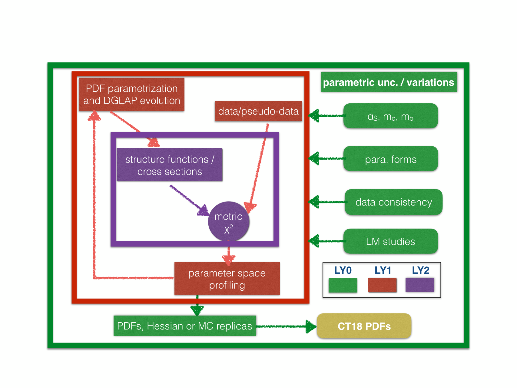
Within the LY1 layer, the calculation of global , or ”layer LY2”, is the core part of the fit that will be repeated for every combination of the PDF parameters. LY2 calculates cross sections for thousands of data points and computes individual for each data set.
Most computational efforts shown in Fig. 72 can be parallelized. For instance, at the LY0 stage, one can simply submit thousands of simultaneous fits with varied inputs to a large computing cluster, since those fits are independent. To obtain a diverse battery of results presented in the CT18(Z) analyses, including the computationally expensive Lagrange Multiplier scans, the high-performance computing clusters at MSU and SMU were used.
At LY1, the major task is to find a global minimum of the in a parameter space with large dimensions (). The choice of the suitable parallelization technique depends strongly on the minimization algorithm. The CT18 analysis uses the variable-metric gradient descent method implemented in the MINUIT package James and Winkler 2004. It involves numerical calculations of the first- and second-order derivatives of , combined with sequential minimum searches along fixed directions in the PDF parameter space. The calculations of derivatives are highly parallelizable, with the CPU-time expenditures scaling with the number of parameters approximately as and , respectively.
In the core part, again the calculation of individual for different data sets, including their cross sections, is now done simultaneously.
While either MPI or OpenMP parallelization protocols are suitable at this stage, the latter is restricted to platforms with shared memory, but required fewer revisions in our fitting code.
Specifically, we used an approach similar to OpenMP to reduce the scope of changes inside our fitting code.
When computing values for the experiments, the fork Linux command splits the main program into multiple threads,
each with a copy of the master memory and carrying out the calculations independently.
Later the join command collects the results from the individual threads and returns them to the main program.
The implementation of this fork-join algorithm is borrowed from the widely-used
CUBA library Hahn 2005 for multi-thread Monte-Carlo integration.
Appendix E Decorrelation of ATLAS jet-production cross-section data
It has been observed in our global analysis, as well as others Harland-Lang et al. 2018, that achieving a robust theoretical description of the Run-1 LHC jet production data generally requires numerical prescriptions to decorrelate select correlated systematic uncertainties. In our work, we follow the recommendations of experimental collaborations in applying such decorrelation procedures.
For example, while the ATLAS 7 TeV inclusive jet production data Aad et al. 2015 (Exp. ID=544) produced an unacceptably high when fitted out of the box, the agreement of data and NNLO theory was improved by applying some decorrelation options proposed by the ATLAS collaboration and summarized in the Appendix of Ref. Aaboud et al. 2017a. The CT18(Z) fits implement ATLAS inclusive jet cross sections defined with an anti- jet algorithm. With this data set, we tested the decorrelation procedures summarized in Table 6 of Ref. Aaboud et al. 2017a and found some to have a substantial impact on the of the ATLAS 7 TeV data. In the end, we followed the specific recommendations of the ATLAS experimentalists themselves, who advocate Malaescu the decorrelation of two jet energy scale (JES) uncertainties, associated with the JES MJB fragmentation (JES16) and the JES flavor response (JES62). We obtained the greatest reduction using the upper portion of Table 6 in Ref. Aaboud et al. 2017a, by decorrelating JES16 and JES62 according to Options 17 and 14 of Table 4, respectively.
Ref. Aaboud et al. 2017a also details decorrelation options for select uncertainties in experimental simulations; of these, we specifically considered the effect of decorrelating the error associated with the nonperturbative correction (‘eNPC’), but found it to have negligible impact on the quality of the CT14 fit according to .
The JES decorrelation that we have implemented proceeds by breaking a given correlated uncertainty into 2-3 subsidiary errors such that their sum in quadrature recovers the original correlated uncertainty. This procedure is bin-dependent; the resulting decorrelated errors depend on the jet’s rapidity and transverse momentum. For example, we decorrelate the JES MJB fragmentation error, , into three components given by
| (61) |
where
| (62) |
and otherwise for or for . We note that Eq. (61) governs the magnitudes of the decorrelated uncertainties, which otherwise inherit the sign of the original uncertainty. A similar algorithm is applied to decorrelate the JES flavor response JES62.
Analogous considerations were applied to the inclusive jet production data sets from CMS 7 and 8 TeV (experiments 542 and 545). Namely, for the 7 TeV CMS jet data, the decorrelation methods of Ref. Khachatryan et al. 2015a were applied to JEC2 with an additional decorrelation88 8 Private communication, M. Voutilainen. for the bin to obtain 6 subsidiary uncertainties. For the 8 TeV CMS jet data, systermatic uncertainties were obtained using the xFitter framework according to the treatment in Ref. Khachatryan et al. 2017c. On the top of that, we found that the residual fluctuations from the Monte-Carlo integration of the available NNLO predictions from NNLOJet Gehrmann-De Ridder et al. 2016a; Gehrmann-De Ridder et al. 2018; Currie et al. 2017a; Currie et al. 2017b lead to elevated for the inclusive jet production experiments, or equivalently, to some uncertainty in the tabulated NNLO/NLO corrections if they are fitted by a smooth function. In the CT18 analysis, the Monte-Carlo (MC) theoretical uncertainty for the three jet experiments is estimated by adding an overall uncorrelated uncertainty (‘MC unc.’) of 0.5%, the typical magnitude of the intrinsic statistical noise associated with Monte-Carlo generation of NNLO/NLO -factors.
Table 11 summarizes the reduction in for the three LHC jet data sets after performing the decorrelation and adding the Monte-Carlo uncertainties, on the example of the CT14 PDFs. For example, for the ATLAS 7 TeV jet data, the decorrelation reduces by units, yet adding the MC uncertainty is still necessary to reduce the to a statistically plausible level (from 1.68 to 1.31 for ).
| evaluated, CT14HERAII NNLO | |||
|---|---|---|---|
| original data | decorr. | 0.5% MC unc. | |
| ATLAS, 7 TeV | 2.34 | 1.68 | 1.31 |
| CMS, 7 TeV | 1.58 | 1.45 | 1.35 |
| CMS, 8 TeV | 1.90 | 1.34 | 1.23 |
Appendix F Hessian profiling of the ATLAS 7 TeV Data
The definitions in xFitter and ePump. As an alternative to directly including new data inside a full QCD global fit, Hessian PDF-profiling techniques provide a fast and flexible approach to explore the impact of new data on a given PDF set; these profiling methods are available within both the xFitter and ePump frameworks. In xFitter, the function includes both experimental and theoretical uncertainties Paukkunen and Zurita 2014; Camarda et al. 2015; xFitter developers 2017:
| (63) |
Here and are the -th experimental datum and corresponding theoretical prediction, respectively, where the index runs over all points in a given experiment. Meanwhile, denotes the total uncorrelated uncertainty, represents the correlated experimental (theoretical) uncertainties, and are the corresponding nuisance parameters. In this case, the index runs over the correlated systematic uncertainties in an experiment, or over the Hessian eigenvector directions of the PDF error sets. Theoretical uncertainties are determined according to predictions based upon the corresponding PDF error sets, , as
| (64) |
in which are the PDF error sets corresponding to positive and negative variations along eigenvector . The tolerance parameter is set to 1 or 1.645 if the PDF error sets are defined at the 68% or 90% C.L., respectively. Instead of scaling down the theoretical uncertainties as in Ref. xFitter developers 2017, we equivalently scale up the corresponding nuisance parameters in order to compare with ePump Schmidt et al. 2018; Hou et al. 2019 more transparently.
The function in Eq. (63) can be converted into the form defined in ePump Schmidt et al. 2018; Hou et al. 2019:
| (65) |
where is the inverse experimental covariance matrix constructed from and Gao et al. 2014. More generally, ePump also contains the option of the so-called “dynamical tolerance” Schmidt et al. 2018; Hou et al. 2019, whose specific value depends on the corresponding PDF eigenvector direction , for the purpose of taking into account additional constraints on the PDF error sets. For example, in the CTEQ-TEA approach, the displacement along a given eigenvector direction is constrained either by the increase in the global by 100 units (at 90% probability level) or by the tier-2 penalty for a too large increase in for one of the experiments Lai et al. 2010b; Gao et al. 2014, which results in a . Dynamical tolerance is applied to MMHT PDFs as well, where separate constraints come from individual experiments Harland-Lang et al. 2015a.
The minimum of the function quantifies the compatibility between theory and data, and the minimization of optimizes the PDFs to describe the data Paukkunen and Zurita 2014; Schmidt et al. 2018. In the linear approximation, the “updated” (or, in the language of xFitter, the “profiled”) central PDF set, , can be given in terms of nuisance parameters, , at the minimum:
| (66) |
The xFitter-profiled PDFs also include second-order diagonal terms, . We note that the off-diagonal terms, for , are not presently included, since the off-diagonal, second-order partial derivatives cannot be constructed solely in terms of Hessian PDF error sets Hou et al. 2017b.
| Program | xFitter | ePump | |||
|---|---|---|---|---|---|
| PDFs | input | profiled | input | ||
| All the 7 measurements, | |||||
| CT14 | 290 | 106 | 285 | 104 | 197 |
| CT18 | 362 | 104 | 356 | 103 | 199 |
| , -peak DY (central), | |||||
| CT14 | 224 | 66 | 220 | 66 | 140 |
| CT18 | 294 | 63 | 289 | 63 | 144 |
Impact of the ATLAS data. Here, we use the Hessian-profiling method of xFitter, as well as ePump updating, to explore the impact of the ATLAS 7 TeV inclusive -production data (Expt. ID=248, Aaboud et al. 2017b) on several PDF sets. The change in the total values before and after profiling/updating with the ATLAS 7 TeV -production data is presented in Table 12 for each PDF set. First, we explore all 7 measurements, having a total of data points: , , neutral current DY in the low-mass, -peak, and high-mass regions for the central and forward selections. In this case, we can directly compare with the ATLAS Aaboud et al. 2017b and MMHT Thorne et al. 2019 analyses. As a second case, we take only the 3 most precise measurements, i.e., the , and -peak DY data for the central selection, with data points in total, which are included in the NNPDF3.1 Ball et al. 2017 and CT18A(Z) global analyses. The comparison of the fitted values for these data in CT18A(Z), NNPDF3.1 and MMHT can be found in Sec. A.3.
Table 12 shows that the values of CT14, before and after xFitter profiling, agree well with the results presented in Ref. Aaboud et al. 2017b. Here, we should apply the tolerance in xFitter as the CT PDFs are defined according to a 90% C.L. Dulat et al. 2016; Hou et al. 2017a. As shown in Ref. Hou et al. 2019, the same results can be reproduced by the ePump code when the tolerance is set to . However, as clearly discussed in Hou et al. 2019, setting in the ePump calculation for the CT PDFs is equivalent to assigning a very large weight (about ) to the new data set included in the fit. xFitter profiling therefore generally overestimates the impact of new data sets when using the CT PDFs. Meanwhile, a universal tolerance value () is not able to capture the constraints of Tier-2 penalty to determine the CT PDF error sets. An appropriate way to update an existing CT PDF set with the inclusion of any new experimental data is to adopt a dynamical tolerance. As such, xFitter profiling yields a smaller value (63) than does ePump updating with a dynamical tolerance (144), as can be seen by comparing the rightmost entries in the last row of Table 12. This conclusion also holds when using xFitter profiling with the MMHT Harland-Lang et al. 2015a and PDF4LHC15 Butterworth et al. 2016 PDFs.
The value of the 34 highest-precision ATLAS 7 TeV -production data points is found to be in the CT18A global fit, cf. Table 9. To this we compare the corresponding value found using ePump updating with dynamical tolerance, for which we obtain , as reported in Table 12. This value includes two distinct contributions, from the difference between theory and data of the ATLAS 7 TeV -production itself, as well as from the quadrature sum of theoretical nuisance parameters, which can be interpreted as the increase in of the other (“prior”) data sets included in the CT18 fit. The large increase in , after ePump updating, indicates the presence of some tensions between the ATLAS 7 TeV -production data and the prior data sets, such as the CCFR/NuTeV SIDIS dimuon data Hou et al. 2019, cf. Fig. 67.
The differences between the values in CT18A (87.6) and from ePump updating with a dynamical tolerance (104) indicate the breakdown of the linear approximation used in the Hessian-updating method, when applied to this case. The breakdown can be confirmed by examining the updated central PDF set. In Fig. 73, we show the gluon and strangeness PDFs at GeV for the CT18 (with 90% C.L. error) and CT18A global fits, compared with ePump dynamical-tolerance updating and xFitter profiling of CT18 with the ATLAS 7 TeV -production data. As compared to the CT18 PDFs, we see that the updated and PDFs from the ePump program are similar to the CT18A PDFs, although with somewhat smaller shifts in the data-sensitive range, . In contrast, the default xFitter profiling produces a much larger shift in both and PDFs, than the CT18A global fit. As a result, xFitter profiling produces a too large change in the -PDF, so that its central prediction touches the upper error band of CT18 at . We have found similar features in the comparison of other flavor PDFs. Namely, the default xFitter program generally overestimates the impact of new data sets in updating the existing PDFs Hou et al. 2019.
| DYNNLO | MCFM | FEWZ | ||||
| xFitter profiling | ||||||
| before | after | before | after | before | after | |
| CT18 | 294 | 63 | 277 | 65 | 225 | 62 |
| CT18A | 87 | – | 92 | – | 109 | – |
| CT18Z | 88 | – | 94 | – | 109 | – |
| ePump dynamic-tolerance updating | ||||||
| CT18 | 289 | 144 | 273 | 144 | 223 | 135 |
| CT18A | 87 | – | 91 | – | 109 | – |
| CT18Z | 88 | – | 94 | – | 109 | – |
Comparison of different NNLO predictions. In addition to the studies described above, we have also used the xFitter and ePump frameworks to examine aspects of the theory calculations for the ATLAS 7 TeV data. In the CT18A(Z) global fits, the NNLO predictions for these measurements were calculated using NNLO/NLO -factors combined with NLO APPLGrid predictions. Specifically, the -factors used in our CT18A(Z) fits were directly extracted from xFitter, where they were calculated with the DYNNLO code Catani and Grazzini 2007; Catani et al. 2009. It was noted by the ATLAS Collaboration in Ref. Aaboud et al. 2017b that the integrated fiducial , and cross sections predicted by the NNLO codes FEWZ Gavin et al. 2011; Gavin et al. 2013; Li and Petriello 2012 and DYNNLO Catani and Grazzini 2007; Catani et al. 2009 differ by about 0.2%, 1.2% and 0.7%, respectively. Fig. 74 shows a slightly larger difference, since the DYNNLO curves include the NLO EW corrections, while other two do not.
Next, we wish to compare various NNLO predictions for differential cross section measurements of the ATLAS 7 TeV -production data. First, we verified that the NLO predictions agree, within 0.2%, among DYNNLO, MCFM Boughezal et al. 2017; Campbell et al. 2015 and FEWZ, which reflects the fact that all three codes adopt the dipole formalism Catani and Seymour 1996; Catani and Seymour 1997 in the NLO calculations. Since the NNLO predictions can be expressed as the NLO predictions multiplied by their -factors, we compare in Fig. 74 the -factors obtained from each code, for every ATLAS 7 TeV -production data point (with 34 data points in total). It can be seen that the differences among the three -factors vary as a function of the -boson rapidity, or the rapidity of the charged lepton from the -boson decay. These differences can be sizable, , as compared to the typically sub-percent statistical uncertainty found in the ATLAS 7 TeV data. We also find that the predictions of MCFM generally lie between those of DYNNLO and FEWZ. This difference can be understood as a consequence of the the different NNLO techniques: FEWZ adopts sector decomposition Binoth and Heinrich 2000; Anastasiou et al. 2004b; Anastasiou et al. 2005, while DYNNLO and MCFM are based on transverse-momentum () Catani and Grazzini 2007; Catani et al. 2009 and -jettiness () Boughezal et al. 2017 subtractions, respectively.
It is also useful to investigate the dependence of the ATLAS 7 TeV fit quality on the specific choice of NNLO calculation scheme. Table 13 summarizes the findings of such a study. After CT18 PDFs are updated using ePump with the ATLAS 7 TeV data, we find that the final value for the ATLAS data set is equal to 144, 144, and 135 units when theory is predicted by the DYNNLO, MCFM and FEWZ NNLO calculations, respectively. Hence, we conclude that these three NNLO calculations lead to fits of similar quality for the ATLAS 7 TeV data. A similar conclusion also holds when using the xFitter framework, with the final values being 63, 65 and 62 units, respectively. To recap, the default xFitter profiling (with tolerance ) overestimates the impact of the ATLAS 7 TeV data when updating the CT18 PDFs, explaining why it yields a smaller value than ePump updating. We also confirm that the updated PDFs by the three -factors differ slightly, but the difference is negligible compared with the same systematical shifts due to the experimental uncertainties. In conclusion, the NNLO theoretical predictions for the ATLAS 7 TeV data by DYNNLO, MCFM and FEWZ show perceptible differences when using the same PDF set. On the other hand, after the PDFs are updated by either ePump and xFitter, the final and PDFs show minor differences among the three codes.
References
- Dulat et al. (2016) S. Dulat, T.-J. Hou, J. Gao, M. Guzzi, J. Huston, P. Nadolsky, J. Pumplin, C. Schmidt, D. Stump, and C.-P. Yuan, Phys. Rev. D93, 033006 (2016), arXiv:1506.07443 [hep-ph] .
- Harland-Lang et al. (2015a) L. A. Harland-Lang, A. D. Martin, P. Motylinski, and R. S. Thorne, Eur. Phys. J. C75, 204 (2015a), arXiv:1412.3989 [hep-ph] .
- Ball et al. (2017) R. D. Ball et al. (NNPDF), Eur. Phys. J. C77, 663 (2017), arXiv:1706.00428 [hep-ph] .
- Alekhin et al. (2017) S. Alekhin, J. Blümlein, S. Moch, and R. Placakyte, Phys. Rev. D96, 014011 (2017), arXiv:1701.05838 [hep-ph] .
- Accardi et al. (2016a) A. Accardi, L. T. Brady, W. Melnitchouk, J. F. Owens, and N. Sato, Phys. Rev. D93, 114017 (2016a), arXiv:1602.03154 [hep-ph] .
- Harland-Lang et al. (2019) L. A. Harland-Lang, A. D. Martin, R. Nathvani, and R. S. Thorne, Eur. Phys. J. C79, 811 (2019), arXiv:1907.02750 [hep-ph] .
- Bertone et al. (2018) V. Bertone, S. Carrazza, N. P. Hartland, and J. Rojo (NNPDF), SciPost Phys. 5, 008 (2018), arXiv:1712.07053 [hep-ph] .
- Manohar et al. (2017) A. V. Manohar, P. Nason, G. P. Salam, and G. Zanderighi, JHEP20 12, 046 (2017), arXiv:1708.01256 [hep-ph] .
- Aad et al. (2015) G. Aad et al. (ATLAS), JHEP 02, 153 (2015), [Erratum: JHEP09,141(2015)], arXiv:1410.8857 [hep-ex] .
- Aaboud et al. (2017a) M. Aaboud et al. (ATLAS), JHEP 09, 020 (2017a), arXiv:1706.03192 [hep-ex] .
- Currie et al. (2017a) J. Currie, E. W. N. Glover, and J. Pires, Phys. Rev. Lett. 118, 072002 (2017a), arXiv:1611.01460 [hep-ph] .
- Currie et al. (2017b) J. Currie, E. W. N. Glover, T. Gehrmann, A. Gehrmann-De Ridder, A. Huss, and J. Pires, Acta Phys. Polon. B48, 955 (2017b), arXiv:1704.00923 [hep-ph] .
- Currie et al. (2018) J. Currie, A. Gehrmann-De Ridder, T. Gehrmann, E. W. N. Glover, A. Huss, and J. Pires, JHEP 10, 155 (2018), arXiv:1807.03692 [hep-ph] .
- Britzger et al. (2012) D. Britzger, K. Rabbertz, F. Stober, and M. Wobisch (fastNLO) (2012) pp. 217–221, arXiv:1208.3641 [hep-ph] .
- Wobisch et al. (2011) M. Wobisch, D. Britzger, T. Kluge, K. Rabbertz, and F. Stober (fastNLO), (2011), arXiv:1109.1310 [hep-ph] .
- Carli et al. (2010) T. Carli, D. Clements, A. Cooper-Sarkar, C. Gwenlan, G. P. Salam, F. Siegert, P. Starovoitov, and M. Sutton, Eur. Phys. J. C66, 503 (2010), arXiv:0911.2985 [hep-ph] .
- Czakon et al. (2017a) M. Czakon, D. Heymes, and A. Mitov, (2017a), arXiv:1704.08551 [hep-ph] .
- (18) http://www.precision.hep.phy.cam.ac.uk/results/ttbar-fastnlo/.
- Thorne et al. (2019) R. S. Thorne, S. Bailey, T. Cridge, L. A. Harland-Lang, A. D. Martin, and R. Nathvani (2019) p. 036, arXiv:1907.08147 [hep-ph] .
- Wang et al. (2018) B.-T. Wang, T. J. Hobbs, S. Doyle, J. Gao, T.-J. Hou, P. M. Nadolsky, and F. I. Olness, Phys. Rev. D98, 094030 (2018), arXiv:1803.02777 [hep-ph] .
- Hobbs et al. (2019) T. J. Hobbs, B.-T. Wang, P. M. Nadolsky, and F. I. Olness, (2019), arXiv:1904.00022 [hep-ph] .
- Pumplin et al. (2001) J. Pumplin, D. Stump, R. Brock, D. Casey, J. Huston, J. Kalk, H.-L. Lai, and W.-K. Tung, Phys. Rev. D65, 014013 (2001), arXiv:hep-ph/0101032 [hep-ph] .
- Pumplin et al. (2002) J. Pumplin, D. R. Stump, J. Huston, H. L. Lai, P. M. Nadolsky, and W.-K. Tung, JHEP 07, 012 (2002), arXiv:hep-ph/0201195 [hep-ph] .
- Schmidt et al. (2018) C. Schmidt, J. Pumplin, and C.-P. Yuan, Phys. Rev. D98, 094005 (2018), arXiv:1806.07950 [hep-ph] .
- Hou et al. (2019) T.-J. Hou, Z. Yu, S. Dulat, C. Schmidt, and C. P. Yuan, (2019), arXiv:1907.12177 [hep-ph] .
- Stump et al. (2001) D. Stump, J. Pumplin, R. Brock, D. Casey, J. Huston, J. Kalk, H.-L. Lai, and W.-K. Tung, Phys. Rev. D65, 014012 (2001), arXiv:hep-ph/0101051 [hep-ph] .
- Tanabashi et al. (2018) M. Tanabashi et al. (Particle Data Group), Phys. Rev. D98, 030001 (2018).
- Lai et al. (2010a) H.-L. Lai, J. Huston, Z. Li, P. Nadolsky, J. Pumplin, D. Stump, and C. P. Yuan, Phys. Rev. D82, 054021 (2010a), arXiv:1004.4624 [hep-ph] .
- Abramowicz et al. (2015) H. Abramowicz et al. (H1, ZEUS), Eur. Phys. J. C75, 580 (2015), arXiv:1506.06042 [hep-ex] .
- Aaron et al. (2010) F. D. Aaron et al. (H1, ZEUS), JHEP 01, 109 (2010), arXiv:0911.0884 [hep-ex] .
- Hou et al. (2017a) T.-J. Hou, S. Dulat, J. Gao, M. Guzzi, J. Huston, P. Nadolsky, J. Pumplin, C. Schmidt, D. Stump, and C. P. Yuan, Phys. Rev. D95, 034003 (2017a), arXiv:1609.07968 [hep-ph] .
- Aaron et al. (2011) F. D. Aaron et al. (H1), Eur. Phys. J. C71, 1579 (2011), arXiv:1012.4355 [hep-ex] .
- Ball et al. (2018) R. D. Ball, V. Bertone, M. Bonvini, S. Marzani, J. Rojo, and L. Rottoli, Eur. Phys. J. C78, 321 (2018), arXiv:1710.05935 [hep-ph] .
- Abdolmaleki et al. (2018) H. Abdolmaleki et al. (xFitter Developers’ Team), Eur. Phys. J. C78, 621 (2018), arXiv:1802.00064 [hep-ph] .
- Abramowicz et al. (2018) H. Abramowicz et al. (H1, ZEUS), Eur. Phys. J. C 78, 473 (2018), arXiv:1804.01019 [hep-ex] .
- Kovařík et al. (2019) K. Kovařík, P. M. Nadolsky, and D. E. Soper, (2019), arXiv:1905.06957 [hep-ph] .
- Lai et al. (2010b) H.-L. Lai, M. Guzzi, J. Huston, Z. Li, P. M. Nadolsky, J. Pumplin, and C. P. Yuan, Phys. Rev. D82, 074024 (2010b), arXiv:1007.2241 [hep-ph] .
- Aaboud et al. (2017b) M. Aaboud et al. (ATLAS), Eur. Phys. J. C77, 367 (2017b), arXiv:1612.03016 [hep-ex] .
- Rojo et al. (2015) J. Rojo et al., J. Phys. G42, 103103 (2015), arXiv:1507.00556 [hep-ph] .
- Alekhin et al. (2015) S. Alekhin et al., Eur. Phys. J. C75, 304 (2015), arXiv:1410.4412 [hep-ph] .
- Gao et al. (2014) J. Gao, M. Guzzi, J. Huston, H.-L. Lai, Z. Li, P. Nadolsky, J. Pumplin, D. Stump, and C. P. Yuan, Phys. Rev. D89, 033009 (2014), arXiv:1302.6246 [hep-ph] .
- Kluge et al. (2006) T. Kluge, K. Rabbertz, and M. Wobisch (2006) pp. 483–486, arXiv:hep-ph/0609285 [hep-ph] .
- Catani and Grazzini (2007) S. Catani and M. Grazzini, Phys. Rev. Lett. 98, 222002 (2007), arXiv:hep-ph/0703012 [hep-ph] .
- Catani et al. (2009) S. Catani, L. Cieri, G. Ferrera, D. de Florian, and M. Grazzini, Phys. Rev. Lett. 103, 082001 (2009), arXiv:0903.2120 [hep-ph] .
- Campbell and Ellis (2010) J. M. Campbell and R. K. Ellis, Nucl. Phys. Proc. Suppl. 205-206, 10 (2010), arXiv:1007.3492 [hep-ph] .
- Boughezal et al. (2017) R. Boughezal, J. M. Campbell, R. K. Ellis, C. Focke, W. Giele, X. Liu, F. Petriello, and C. Williams, Eur. Phys. J. C77, 7 (2017), arXiv:1605.08011 [hep-ph] .
- Campbell et al. (2015) J. M. Campbell, R. K. Ellis, and W. T. Giele, Eur. Phys. J. C75, 246 (2015), arXiv:1503.06182 [physics.comp-ph] .
- Gavin et al. (2011) R. Gavin, Y. Li, F. Petriello, and S. Quackenbush, Comput. Phys. Commun. 182, 2388 (2011), arXiv:1011.3540 [hep-ph] .
- Gavin et al. (2013) R. Gavin, Y. Li, F. Petriello, and S. Quackenbush, Comput. Phys. Commun. 184, 208 (2013), arXiv:1201.5896 [hep-ph] .
- Li and Petriello (2012) Y. Li and F. Petriello, Phys. Rev. D86, 094034 (2012), arXiv:1208.5967 [hep-ph] .
- Gehrmann-De Ridder et al. (2016a) A. Gehrmann-De Ridder, T. Gehrmann, E. W. N. Glover, A. Huss, and T. A. Morgan, Phys. Rev. Lett. 117, 022001 (2016a), arXiv:1507.02850 [hep-ph] .
- Gehrmann-De Ridder et al. (2018) A. Gehrmann-De Ridder, T. Gehrmann, E. W. N. Glover, A. Huss, and D. M. Walker, Phys. Rev. Lett. 120, 122001 (2018), arXiv:1712.07543 [hep-ph] .
- Ladinsky and Yuan (1994) G. A. Ladinsky and C.-P. Yuan, Phys. Rev. D50, R4239 (1994), arXiv:hep-ph/9311341 [hep-ph] .
- Balazs and Yuan (1997) C. Balazs and C.-P. Yuan, Phys. Rev. D56, 5558 (1997), arXiv:hep-ph/9704258 [hep-ph] .
- Nadolsky and Sullivan (2001) P. M. Nadolsky and Z. Sullivan, eConf C010630, P510 (2001), arXiv:hep-ph/0110378 [hep-ph] .
- Nadolsky et al. (2008) P. M. Nadolsky, H.-L. Lai, Q.-H. Cao, J. Huston, J. Pumplin, D. Stump, W.-K. Tung, and C. P. Yuan, Phys. Rev. D78, 013004 (2008), arXiv:0802.0007 [hep-ph] .
- Seligman (1997) W. G. Seligman, Ph.D. thesis, Nevis Labs, Columbia U. (1997).
- Yang et al. (1996) U.-K. Yang et al. (CCFR/NuTeV), J. Phys. G22, 775 (1996), arXiv:hep-ex/9605005 [hep-ex] .
- Aaij et al. (2012) R. Aaij et al. (LHCb), JHEP 06, 058 (2012), arXiv:1204.1620 [hep-ex] .
- Aad et al. (2012a) G. Aad et al. (ATLAS), Phys. Rev. D86, 014022 (2012a), arXiv:1112.6297 [hep-ex] .
- Chatrchyan et al. (2013a) S. Chatrchyan et al. (CMS), Phys. Rev. D87, 112002 (2013a), [Erratum: Phys. Rev.D87,no.11,119902(2013)], arXiv:1212.6660 [hep-ex] .
- Benvenuti et al. (1989) A. C. Benvenuti et al. (BCDMS), Phys. Lett. B223, 485 (1989).
- Benvenuti et al. (1990) A. C. Benvenuti et al. (BCDMS), Phys. Lett. B237, 592 (1990).
- Arneodo et al. (1997) M. Arneodo et al. (New Muon), Nucl. Phys. B483, 3 (1997), arXiv:hep-ph/9610231 [hep-ph] .
- Berge et al. (1991) J. P. Berge et al., Z. Phys. C49, 187 (1991).
- Yang et al. (2001) U.-K. Yang et al. (CCFR/NuTeV), Phys. Rev. Lett. 86, 2742 (2001), arXiv:hep-ex/0009041 [hep-ex] .
- Seligman et al. (1997) W. G. Seligman et al., Phys. Rev. Lett. 79, 1213 (1997), arXiv:hep-ex/9701017 [hep-ex] .
- Mason (2006) D. A. Mason, Ph.D. thesis, Oregon U. (2006).
- Goncharov et al. (2001) M. Goncharov et al. (NuTeV), Phys. Rev. D64, 112006 (2001), arXiv:hep-ex/0102049 [hep-ex] .
- Aktas et al. (2005) A. Aktas et al. (H1), Eur. Phys. J. C40, 349 (2005), arXiv:hep-ex/0411046 [hep-ex] .
- Abramowicz et al. (2013) H. Abramowicz et al. (ZEUS, H1), Eur. Phys. J. C73, 2311 (2013), arXiv:1211.1182 [hep-ex] .
- Moreno et al. (1991) G. Moreno et al., Phys. Rev. D43, 2815 (1991).
- Towell et al. (2001) R. S. Towell et al. (NuSea), Phys. Rev. D64, 052002 (2001), arXiv:hep-ex/0103030 [hep-ex] .
- Webb et al. (2003) J. C. Webb et al. (NuSea), (2003), arXiv:hep-ex/0302019 [hep-ex] .
- Abe et al. (1998) F. Abe et al. (CDF), Phys. Rev. Lett. 81, 5754 (1998), arXiv:hep-ex/9809001 .
- Acosta et al. (2005) D. Acosta et al. (CDF), Phys. Rev. D71, 051104 (2005), arXiv:hep-ex/0501023 [hep-ex] .
- Abazov et al. (2008a) V. M. Abazov et al. (D0), Phys. Rev. D77, 011106 (2008a), arXiv:0709.4254 [hep-ex] .
- Abazov et al. (2007) V. Abazov et al. (D0), Phys. Rev. D 76, 012003 (2007), arXiv:hep-ex/0702025 .
- Aaltonen et al. (2010) T. A. Aaltonen et al. (CDF), Phys. Lett. B692, 232 (2010), arXiv:0908.3914 [hep-ex] .
- Chatrchyan et al. (2014a) S. Chatrchyan et al. (CMS), Phys. Rev. D90, 032004 (2014a), arXiv:1312.6283 [hep-ex] .
- Chatrchyan et al. (2012) S. Chatrchyan et al. (CMS), Phys. Rev. Lett. 109, 111806 (2012), arXiv:1206.2598 [hep-ex] .
- Aad et al. (2012b) G. Aad et al. (ATLAS), Phys. Rev. D85, 072004 (2012b), arXiv:1109.5141 [hep-ex] .
- Abazov et al. (2015) V. M. Abazov et al. (D0), Phys. Rev. D91, 032007 (2015), [Erratum: Phys. Rev.D91,no.7,079901(2015)], arXiv:1412.2862 [hep-ex] .
- Aaltonen et al. (2008) T. Aaltonen et al. (CDF), Phys. Rev. D78, 052006 (2008), [Erratum: Phys. Rev.D79,119902(2009)], arXiv:0807.2204 [hep-ex] .
- Abazov et al. (2008b) V. M. Abazov et al. (D0), Phys. Rev. Lett. 101, 062001 (2008b), arXiv:0802.2400 [hep-ex] .
- Dulat et al. (2014) S. Dulat, T.-J. Hou, J. Gao, J. Huston, J. Pumplin, C. Schmidt, D. Stump, and C. P. Yuan, Phys. Rev. D89, 073004 (2014), arXiv:1309.0025 [hep-ph] .
- Aaij et al. (2015a) R. Aaij et al. (LHCb), JHEP 08, 039 (2015a), arXiv:1505.07024 [hep-ex] .
- Aaij et al. (2015b) R. Aaij et al. (LHCb), JHEP 05, 109 (2015b), arXiv:1503.00963 [hep-ex] .
- Khachatryan et al. (2016) V. Khachatryan et al. (CMS), Eur. Phys. J. C76, 469 (2016), arXiv:1603.01803 [hep-ex] .
- Aaij et al. (2016) R. Aaij et al. (LHCb), JHEP 01, 155 (2016), arXiv:1511.08039 [hep-ex] .
- Aad et al. (2016a) G. Aad et al. (ATLAS), Eur. Phys. J. C76, 291 (2016a), arXiv:1512.02192 [hep-ex] .
- Chatrchyan et al. (2014b) S. Chatrchyan et al. (CMS), Phys. Rev. D90, 072006 (2014b), arXiv:1406.0324 [hep-ex] .
- Khachatryan et al. (2017a) V. Khachatryan et al. (CMS), JHEP 03, 156 (2017a), arXiv:1609.05331 [hep-ex] .
- Sirunyan et al. (2017) A. M. Sirunyan et al. (CMS), Eur. Phys. J. C77, 459 (2017), arXiv:1703.01630 [hep-ex] .
- Aad et al. (2016b) G. Aad et al. (ATLAS), Eur. Phys. J. C76, 538 (2016b), arXiv:1511.04716 [hep-ex] .
- Khachatryan et al. (2015a) V. Khachatryan et al. (CMS), Eur. Phys. J. C75, 288 (2015a), arXiv:1410.6765 [hep-ex] .
- (97) M. Voutilainen, Private communication (2018).
- Amat et al. (2019) O. Amat et al., PoS DIS2019, 017 (2019).
- Bailey and Harland-Lang (2019) S. Bailey and L. Harland-Lang, (2019), arXiv:1909.10541 [hep-ph] .
- (100) B. Malaescu, Private communication (2018).
- Kadir et al. (2020) M. Kadir, A. Ablet, S. Dulat, T.-J. Hou, I. Sitiwaldi, and A. Tursun, (2020), arXiv:2003.13740 [hep-ph] .
- Sirunyan et al. (2019) A. M. Sirunyan et al. (CMS), JHEP 02, 149 (2019), arXiv:1811.06625 [hep-ex] .
- Aad et al. (2014a) G. Aad et al. (ATLAS), JHEP 09, 145 (2014a), arXiv:1406.3660 [hep-ex] .
- Khachatryan et al. (2015b) V. Khachatryan et al. (CMS), Phys. Lett. B749, 187 (2015b), arXiv:1504.03511 [hep-ex] .
- Khachatryan et al. (2017b) V. Khachatryan et al. (CMS), JHEP 02, 096 (2017b), arXiv:1606.05864 [hep-ex] .
- Aad et al. (2016c) G. Aad et al. (ATLAS), JHEP 08, 009 (2016c), arXiv:1606.01736 [hep-ex] .
- Aad et al. (2013) G. Aad et al. (ATLAS), Phys. Lett. B725, 223 (2013), arXiv:1305.4192 [hep-ex] .
- Aad et al. (2014b) G. Aad et al. (ATLAS), JHEP 06, 112 (2014b), arXiv:1404.1212 [hep-ex] .
- Aad et al. (2014c) G. Aad et al. (ATLAS), JHEP 05, 068 (2014c), arXiv:1402.6263 [hep-ex] .
- Chatrchyan et al. (2014c) S. Chatrchyan et al. (CMS), JHEP 02, 013 (2014c), arXiv:1310.1138 [hep-ex] .
- Chatrchyan et al. (2013b) S. Chatrchyan et al. (CMS), JHEP 12, 030 (2013b), arXiv:1310.7291 [hep-ex] .
- Khachatryan et al. (2015c) V. Khachatryan et al. (CMS), Eur. Phys. J. C75, 147 (2015c), arXiv:1412.1115 [hep-ex] .
- Golec-Biernat and Wusthoff (1998) K. J. Golec-Biernat and M. Wusthoff, Phys. Rev. D59, 014017 (1998), arXiv:hep-ph/9807513 [hep-ph] .
- Caola et al. (2010) F. Caola, S. Forte, and J. Rojo, Phys. Lett. B686, 127 (2010), arXiv:0910.3143 [hep-ph] .
- Guzzi et al. (2012) M. Guzzi, P. M. Nadolsky, H.-L. Lai, and C. P. Yuan, Phys. Rev. D86, 053005 (2012), arXiv:1108.5112 [hep-ph] .
- Aivazis et al. (1994a) M. A. G. Aivazis, J. C. Collins, F. I. Olness, and W.-K. Tung, Phys. Rev. D50, 3102 (1994a), arXiv:hep-ph/9312319 [hep-ph] .
- Aivazis et al. (1994b) M. A. G. Aivazis, F. I. Olness, and W.-K. Tung, Phys. Rev. D50, 3085 (1994b), arXiv:hep-ph/9312318 [hep-ph] .
- Kramer et al. (2000) M. Kramer, 1, F. I. Olness, and D. E. Soper, Phys. Rev. D62, 096007 (2000), arXiv:hep-ph/0003035 [hep-ph] .
- Tung et al. (2002) W.-K. Tung, S. Kretzer, and C. Schmidt, J. Phys. G28, 983 (2002), arXiv:hep-ph/0110247 [hep-ph] .
- Gao et al. (2013) J. Gao, M. Guzzi, and P. M. Nadolsky, Eur. Phys. J. C73, 2541 (2013), arXiv:1304.3494 [hep-ph] .
- Berger et al. (2016) E. L. Berger, J. Gao, C. S. Li, Z. L. Liu, and H. X. Zhu, Phys. Rev. Lett. 116, 212002 (2016), arXiv:1601.05430 [hep-ph] .
- Nagy (2003) Z. Nagy, Phys. Rev. D68, 094002 (2003), arXiv:hep-ph/0307268 [hep-ph] .
- Bertone et al. (2014) V. Bertone, R. Frederix, S. Frixione, J. Rojo, and M. Sutton, JHEP 08, 166 (2014), arXiv:1406.7693 [hep-ph] .
- Buza and van Neerven (1997) M. Buza and W. van Neerven, Nucl. Phys. B 500, 301 (1997), arXiv:hep-ph/9702242 .
- Czakon et al. (2017b) M. Czakon, D. Heymes, and A. Mitov, JHEP 04, 071 (2017b), arXiv:1606.03350 [hep-ph] .
- Czakon et al. (2018) M. Czakon, A. Ferroglia, D. Heymes, A. Mitov, B. D. Pecjak, D. J. Scott, X. Wang, and L. L. Yang, JHEP 05, 149 (2018), arXiv:1803.07623 [hep-ph] .
- Anastasiou et al. (2004a) C. Anastasiou, L. J. Dixon, K. Melnikov, and F. Petriello, Phys. Rev. D69, 094008 (2004a), arXiv:hep-ph/0312266 [hep-ph] .
- Anastasiou et al. (2003) C. Anastasiou, L. J. Dixon, K. Melnikov, and F. Petriello, Phys. Rev. Lett. 91, 182002 (2003), arXiv:hep-ph/0306192 [hep-ph] .
- Konychev and Nadolsky (2006) A. V. Konychev and P. M. Nadolsky, Phys. Lett. B633, 710 (2006), arXiv:hep-ph/0506225 [hep-ph] .
- Bellm et al. (2019) J. Bellm et al., (2019), arXiv:1903.12563 [hep-ph] .
- Dittmaier et al. (2012) S. Dittmaier, A. Huss, and C. Speckner, JHEP 11, 095 (2012), arXiv:1210.0438 [hep-ph] .
- Alwall et al. (2014) J. Alwall, R. Frederix, S. Frixione, V. Hirschi, F. Maltoni, O. Mattelaer, H. S. Shao, T. Stelzer, P. Torrielli, and M. Zaro, JHEP 07, 079 (2014), arXiv:1405.0301 [hep-ph] .
- Hollik et al. (2015) W. Hollik, B. A. Kniehl, E. S. Scherbakova, and O. L. Veretin, Nucl. Phys. B900, 576 (2015), arXiv:1504.07574 [hep-ph] .
- Kallweit et al. (2015) S. Kallweit, J. M. Lindert, S. Pozzorini, M. Schönherr, and P. Maierhöfer (2015) pp. 121–124, arXiv:1505.05704 [hep-ph] .
- Czakon et al. (2017c) M. Czakon, D. Heymes, A. Mitov, D. Pagani, I. Tsinikos, and M. Zaro, JHEP 10, 186 (2017c), arXiv:1705.04105 [hep-ph] .
- (136) http://www.precision.hep.phy.cam.ac.uk/results/ttbar-nnloqcd-nloew/.
- Moch et al. (2004) S. Moch, J. A. M. Vermaseren, and A. Vogt, Nucl. Phys. B688, 101 (2004), arXiv:hep-ph/0403192 [hep-ph] .
- Vogt et al. (2004) A. Vogt, S. Moch, and J. A. M. Vermaseren, Nucl. Phys. B691, 129 (2004), arXiv:hep-ph/0404111 [hep-ph] .
- Ablinger et al. (2014) J. Ablinger, A. Behring, J. Blümlein, A. De Freitas, A. von Manteuffel, and C. Schneider, Nucl. Phys. B890, 48 (2014), arXiv:1409.1135 [hep-ph] .
- Ablinger et al. (2017) J. Ablinger, A. Behring, J. Blümlein, A. De Freitas, A. von Manteuffel, and C. Schneider, Nucl. Phys. B922, 1 (2017), arXiv:1705.01508 [hep-ph] .
- Stump et al. (2003) D. Stump, J. Huston, J. Pumplin, W.-K. Tung, H. Lai, S. Kuhlmann, and J. Owens, JHEP 10, 046 (2003), arXiv:hep-ph/0303013 .
- Ball et al. (2013) R. D. Ball et al., JHEP 04, 125 (2013), arXiv:1211.5142 [hep-ph] .
- D’Agostini (1994) G. D’Agostini, Nucl. Instrum. Meth. A 346, 306 (1994).
- D’Agostini (1999) G. D’Agostini, “Bayesian reasoning in high-energy physics: Principles and applications,” (1999).
- Lai et al. (2007) H.-L. Lai, P. M. Nadolsky, J. Pumplin, D. Stump, W.-K. Tung, and C. P. Yuan, JHEP 04, 089 (2007), arXiv:hep-ph/0702268 [hep-ph] .
- Olness et al. (2005) F. Olness, J. Pumplin, D. Stump, J. Huston, P. M. Nadolsky, H.-L. Lai, S. Kretzer, J. F. Owens, and W.-K. Tung, Eur. Phys. J. C40, 145 (2005), arXiv:hep-ph/0312323 [hep-ph] .
- Ball et al. (2012) R. D. Ball, V. Bertone, L. Del Debbio, S. Forte, A. Guffanti, J. I. Latorre, S. Lionetti, J. Rojo, and M. Ubiali, Phys. Lett. B707, 66 (2012), arXiv:1110.2483 [hep-ph] .
- Harland-Lang et al. (2015b) L. A. Harland-Lang, A. D. Martin, P. Motylinski, and R. S. Thorne, Eur. Phys. J. C75, 435 (2015b), arXiv:1506.05682 [hep-ph] .
- Hou et al. (2018) T.-J. Hou, S. Dulat, J. Gao, M. Guzzi, J. Huston, P. Nadolsky, C. Schmidt, J. Winter, K. Xie, and C. P. Yuan, JHEP 02, 059 (2018), arXiv:1707.00657 [hep-ph] .
- Hou et al. (2017b) T.-J. Hou et al., JHEP 03, 099 (2017b), arXiv:1607.06066 [hep-ph] .
- Butterworth et al. (2016) J. Butterworth et al., J. Phys. G43, 023001 (2016), arXiv:1510.03865 [hep-ph] .
- Lin et al. (2018) H.-W. Lin et al., Prog. Part. Nucl. Phys. 100, 107 (2018), arXiv:1711.07916 [hep-ph] .
- Constantinou et al. (2020) M. Constantinou et al., (2020), arXiv:2006.08636 [hep-ph] .
- Amaudruz et al. (1991) P. Amaudruz et al. (New Muon), Phys. Rev. Lett. 66, 2712 (1991).
- Arneodo et al. (1994) M. Arneodo et al. (New Muon), Phys. Rev. D50, R1 (1994).
- Gottfried (1967) K. Gottfried, Phys. Rev. Lett. 18, 1174 (1967).
- Alexandrou et al. (2020) C. Alexandrou, S. Bacchio, M. Constantinou, J. Finkenrath, K. Hadjiyiannakou, K. Jansen, G. Koutsou, H. Panagopoulos, and G. Spanoudes, Phys. Rev. D 101, 094513 (2020), arXiv:2003.08486 [hep-lat] .
- Yang et al. (2018a) Y.-B. Yang, J. Liang, Y.-J. Bi, Y. Chen, T. Draper, K.-F. Liu, and Z. Liu, Phys. Rev. Lett. 121, 212001 (2018a), arXiv:1808.08677 [hep-lat] .
- Yang et al. (2018b) Y.-B. Yang, M. Gong, J. Liang, H.-W. Lin, K.-F. Liu, D. Pefkou, and P. Shanahan, Phys. Rev. D 98, 074506 (2018b), arXiv:1805.00531 [hep-lat] .
- Deka et al. (2009) M. Deka, T. Streuer, T. Doi, S. J. Dong, T. Draper, K. F. Liu, N. Mathur, and A. W. Thomas, Phys. Rev. D79, 094502 (2009), arXiv:0811.1779 [hep-ph] .
- Liang et al. (2019) J. Liang, M. Sun, Y.-B. Yang, T. Draper, and K.-F. Liu, (2019), arXiv:1901.07526 [hep-ph] .
- Gockeler et al. (2005) M. Gockeler, R. Horsley, D. Pleiter, P. E. L. Rakow, and G. Schierholz (QCDSF), Phys. Rev. D71, 114511 (2005), arXiv:hep-ph/0410187 [hep-ph] .
- Dolgov et al. (2002) D. Dolgov et al. (LHPC, TXL), Phys. Rev. D66, 034506 (2002), arXiv:hep-lat/0201021 [hep-lat] .
- Gockeler et al. (1996) M. Gockeler, R. Horsley, E.-M. Ilgenfritz, H. Perlt, P. E. L. Rakow, G. Schierholz, and A. Schiller, Phys. Rev. D53, 2317 (1996), arXiv:hep-lat/9508004 [hep-lat] .
- Martin et al. (2009) A. D. Martin, W. J. Stirling, R. S. Thorne, and G. Watt, Eur. Phys. J. C63, 189 (2009), arXiv:0901.0002 [hep-ph] .
- (166) CTEQ-TEA, https://ct.hepforge.org/PDFs/ct18/figures/L2Sensitivity/.
- Gehrmann-De Ridder et al. (2016b) A. Gehrmann-De Ridder, T. Gehrmann, E. W. N. Glover, A. Huss, and T. A. Morgan, JHEP 11, 094 (2016b), [Erratum: JHEP10,126(2018)], arXiv:1610.01843 [hep-ph] .
- Gehrmann-De Ridder et al. (2016c) A. Gehrmann-De Ridder, T. Gehrmann, E. W. N. Glover, A. Huss, and T. A. Morgan, PoS LL2016, 056 (2016c), arXiv:1607.01749 [hep-ph] .
- Gehrmann-De Ridder et al. (2016d) A. Gehrmann-De Ridder, T. Gehrmann, N. Glover, A. Huss, and T. A. Morgan, PoS RADCOR2015, 075 (2016d), arXiv:1601.04569 [hep-ph] .
- Gehrmann-De Ridder et al. (2016e) A. Gehrmann-De Ridder, T. Gehrmann, E. W. N. Glover, A. Huss, and T. A. Morgan, JHEP 07, 133 (2016e), arXiv:1605.04295 [hep-ph] .
- Forte and Kassabov (2020) S. Forte and Z. Kassabov, Eur. Phys. J. C 80, 182 (2020), arXiv:2001.04986 [hep-ph] .
- Czakon et al. (2019) M. Czakon, S. Dulat, T.-J. Hou, J. Huston, A. Mitov, A. S. Papanastasiou, I. Sitiwaldi, Z. Yu, and C. P. Yuan, “A study of the impact of double-differential top distributions from CMS on parton distribution functions,” (2019), arXiv:1912.08801 [hep-ph] .
- Gottschalk (1981) T. Gottschalk, Phys. Rev. D23, 56 (1981).
- Gluck et al. (1997) M. Gluck, S. Kretzer, and E. Reya, Phys. Lett. B398, 381 (1997), [Erratum: Phys. Lett.B405,392(1997)], arXiv:hep-ph/9701364 [hep-ph] .
- Blumlein et al. (2011) J. Blumlein, A. Hasselhuhn, P. Kovacikova, and S. Moch, Phys. Lett. B700, 294 (2011), arXiv:1104.3449 [hep-ph] .
- Collins (1998) J. C. Collins, Phys. Rev. D58, 094002 (1998), arXiv:hep-ph/9806259 [hep-ph] .
- Gao (2018) J. Gao, JHEP 02, 026 (2018), arXiv:1710.04258 [hep-ph] .
- Ball et al. (2019) R. D. Ball, E. R. Nocera, and R. L. Pearson (NNPDF), Eur. Phys. J. C 79, 282 (2019), arXiv:1812.09074 [hep-ph] .
- Arbuzov et al. (2016) A. Arbuzov, D. Bardin, S. Bondarenko, P. Christova, L. Kalinovskaya, U. Klein, V. Kolesnikov, L. Rumyantsev, R. Sadykov, and A. Sapronov, JETP Lett. 103, 131 (2016), arXiv:1509.03052 [hep-ph] .
- Aad et al. (2016d) G. Aad et al. (ATLAS), JHEP 08, 009 (2016d), arXiv:1606.01736 [hep-ex] .
- Aidala et al. (2019) C. A. Aidala et al. (SeaQuest), Nucl. Instrum. Meth. A930, 49 (2019), arXiv:1706.09990 [physics.ins-det] .
- Czakon et al. (2013) M. Czakon, P. Fiedler, and A. Mitov, Phys. Rev. Lett. 110, 252004 (2013), arXiv:1303.6254 [hep-ph] .
- Czakon and Mitov (2014) M. Czakon and A. Mitov, Comput. Phys. Commun. 185, 2930 (2014), arXiv:1112.5675 [hep-ph] .
- Anastasiou et al. (2011) C. Anastasiou, S. Buehler, F. Herzog, and A. Lazopoulos, JHEP 12, 058 (2011), arXiv:1107.0683 [hep-ph] .
- (185) Joshua Isaacson, Bin Yan and C.-P. Yuan, “ResBos-2: Precision Resummation for the LHC Era,” in preparation.
- Yalkun and Dulat (2019) N. Yalkun and S. Dulat, Chin. Phys. C43, 123101 (2019), arXiv:1908.00026 [hep-ph] .
- Accardi et al. (2016b) A. Accardi et al., Eur. Phys. J. A52, 268 (2016b), arXiv:1212.1701 [nucl-ex] .
- (188) CT18PDFs, https://hep.pa.msu.edu/cteq/public/ct18.html and https://tinyurl.com/ct18pdfs-1.
- (189) LHAPDF6, https://lhapdf.hepforge.org/.
- (190) LHAPDF5, http://hep.pa.msu.edu/cteq/public/ct14/lhapdf/v5/.
- Collins and Pumplin (2001) J. C. Collins and J. Pumplin, “Tests of goodness of fit to multiple data sets,” (2001), arXiv:hep-ph/0105207 [hep-ph] .
- Barone et al. (2000) V. Barone, C. Pascaud, and F. Zomer, Eur. Phys. J. C12, 243 (2000), arXiv:hep-ph/9907512 [hep-ph] .
- Alekhin et al. (2018) S. Alekhin, J. Blümlein, and S. Moch, Phys. Lett. B777, 134 (2018), arXiv:1708.01067 [hep-ph] .
- James and Winkler (2004) F. James and M. Winkler, http://seal.web.cern.ch/seal/documents/minuit/mnusersguide.pdf (2004).
- Hahn (2005) T. Hahn, Comput. Phys. Commun. 168, 78 (2005), arXiv:hep-ph/0404043 [hep-ph] .
- Harland-Lang et al. (2018) L. A. Harland-Lang, A. D. Martin, and R. S. Thorne, Eur. Phys. J. C78, 248 (2018), arXiv:1711.05757 [hep-ph] .
- Khachatryan et al. (2017c) V. Khachatryan et al. (CMS), JINST 12, P02014 (2017c), arXiv:1607.03663 [hep-ex] .
- Paukkunen and Zurita (2014) H. Paukkunen and P. Zurita, JHEP 12, 100 (2014), arXiv:1402.6623 [hep-ph] .
- Camarda et al. (2015) S. Camarda et al. (HERAFitter developers’ Team), Eur. Phys. J. C75, 458 (2015), arXiv:1503.05221 [hep-ph] .
- xFitter developers (2017) xFitter developers, https://www.xfitter.org/xFitter/xFitter/DownloadPage?action=AttachFile&do=view&target=manual.pdf (2017).
- Catani and Seymour (1996) S. Catani and M. H. Seymour, Phys. Lett. B378, 287 (1996), arXiv:hep-ph/9602277 [hep-ph] .
- Catani and Seymour (1997) S. Catani and M. H. Seymour, Nucl. Phys. B485, 291 (1997), [Erratum: Nucl. Phys.B510,503(1998)], arXiv:hep-ph/9605323 [hep-ph] .
- Binoth and Heinrich (2000) T. Binoth and G. Heinrich, Nucl. Phys. B585, 741 (2000), arXiv:hep-ph/0004013 [hep-ph] .
- Anastasiou et al. (2004b) C. Anastasiou, K. Melnikov, and F. Petriello, Phys. Rev. D69, 076010 (2004b), arXiv:hep-ph/0311311 [hep-ph] .
- Anastasiou et al. (2005) C. Anastasiou, K. Melnikov, and F. Petriello, Nucl. Phys. B724, 197 (2005), arXiv:hep-ph/0501130 [hep-ph] .
Appendix G Supplemental Material
G.1 Additional comparisons between PDF sets


G.2 Additional histograms and comparisons to data
The residuals and nuisance parameters for Exp. ID=249 are shown in Fig. 85. Both are reasonably compatible with the normal distribution with mean 0 and standard deviation 1.
The overall quality of the fit to the combined LHC jet data is demonstrated by the distributions of residuals and the fitted values of nuisance parameters, shown in Figs. 86 and 87.