First-order and continuous quantum phase transitions in the anisotropic quantum Rabi-Stark model
Abstract
Various quantum phase transitions in the anisotropic Rabi-Stark model with both the nonlinear Stark coupling and the linear dipole coupling between a two-level system and a single-mode cavity are studied in this work. The first-order quantum phase transitions are detected by the level crossing of the ground-state and the first-excited state with the help of the pole structure of the transcendental functions derived by the Bogoliubov operators approach. As the nonlinear Stark coupling is the same as the cavity frequency, this model can be solved by mapping to an effective quantum oscillator. All energy levels close at the critical coupling in this case, indicating continuous quantum phase transitions. The critical gap exponent is independent of the anisotropy as long as the counter-rotating wave coupling is present, but essentially changed if the counter-rotating wave coupling disappears completely. It is suggested that the gapless Goldstone mode excitations could appear above a critical coupling in the present model in the rotating-wave approximation.
pacs
03.65.Yz, 03.65.Ud, 71.27.+a, 71.38.kI Introduction
The quantum Rabi model (QRM) describes the basic interaction between a two-level (artificial) atom and a one-mode bosonic cavity Rabi; Braak2 and is a paradigmatic model in quantum optics. In conventional cavity quantum electrodynamics (QED) systems, due to the extremely weak coupling between the two-level systems and the cavity, the basic physics can be explored in the rotating wave approximation (RWA) JC; book. However, the situation has changed in the past decade. In many advanced solid devices, such as the superconducting circuit QED systems Niemczyk; Forn1 and trapped ions Leibfried; Clarke, the ultrastrong coupling even deep strong coupling Forn2; Yoshihara between the artificial atom and the resonators have been accessed, and the RWA is demonstrated invalid Niemczyk. On the other hand, the two-level system appearing in these systems is just a qubit, which is the building block of quantum information technologies with the ultimate goal being to realize quantum algorithms and quantum computations. Just motivated by the experimental advances and potential applications in quantum information technologies, the QRM has attracted extensive attentions theoretically, especially for the analytical solutions Casanova; chenqh; Braak; Chen2012; Chen2; Zhong; zheng; luo2 and the quantum phase transition (QPT) plenio; hgluo. For a more complete review, please refer to Refs. ReviewF; Kockum; Boit.
The QRM continues to inspire exciting developments in both experiments and theories recently. The anisotropic QRM yejw2013; Fanheng; Tomka was motivated by the recent experimental progress Wallraff; Schiroa; Erlingsson. It can be mapped onto the model describing a two-dimensional electron gas with Rashba ( rotating wave coupling relevant) and Dresselhaus ( counter rotating-wave coupling dependent) spin-orbit couplings subject to a perpendicular magnetic field Erlingsson. These couplings can be tuned by an applied electric and magnetic field, allowing the exploration of the whole parameter space of the model. This model can directly emerge in both cavity QED Schiroa and circuit QED Wallraff. Interestingly, the first-order QPT is observed in the anisotropic QRM Fanheng and the Jaynes-Cummings model puhan.
On the other hand, Grimsmo and Parkins proposed a scheme by adding a nonlinear coupling term to the QRM Hamiltonian Grimsmo1; Grimsmo2. This nonlinear coupling term has been discussed in the quantum optics literature under the name of dynamical Stark shift, a quantum version of the Bloch-Siegert shift, so it was later named the quantum Rabi-Stark model (RSM) Eckle. This model has also attracted much attention in recent years Maciejewski; Xie; Xie2; Cong. More recently, the anisotropic Dicke model with the Stark coupling terms, which can be called as anisotropic Dicke-Stark model, was demonstrated via cavity assisted Raman transitions in a configuration using counterpropagating laser beams zhiqiang. For the one-atom case, it is just the anisotropic Rabi-Stark model (ARSM).
Actually, the implementation of the ARSM has been also demonstrated most recently in a trapped ion Cong. In this proposal, external laser beams are applied to induce an interaction between an electronic transition and the motional degree of freedom, thus the Stark term is generated. The anisotropic coupling strengths are determined by laser field amplitudes of the red-sideband and blue-sideband driving lasers, which can be tuned independently in the trapped ion experimental system.
Theoretically, the RSM has been studied by the Bargmann space approach Eckle; Maciejewski. Later it was solved by the Bogoliubov operator approach (BOA) Xie. Many exotic properties are found within the analytic exact solutions, such as the first-order QPT and the spectra collapse Xie. Then what are the properties contained in the ARSM? Especially, since the first-order QPT occur in the anisotropic QRM and the RSM, while the continuous QPTs are present in the isotropic QRM, rich QPTs might appear in this generalized model due to more tunable interaction constants in the wide parameter space.
The paper is organized as follows. In Sec. II, we first describe the ARSM briefly, and then demonstrate that eigensolutions can then be easily obtained by the zeros of the transcendant function derived by the BOA. In Sec. III, the first-order QPT is analyzed based on the level crossing of the ground-state and the first-excited state, based on the pole structure of the derived transcendant function. In Sec. IV, the energy gap near the critical coupling for the nonlinear Stark coupling being the same as the cavity frequency is calculated analytically by the exact mapping the ARSM to a quantum oscillator. The energy-gap exponents are also obtained. The last section contains some concluding remarks. Details of the solutions to the ARSM in the two cases are deferred to the Appendixes.
II Model and solutions
The Hamiltonian of the ARSM reads
| (1) | |||||
where is qubit energy difference, is the photonic creation (annihilation) operator of the single-mode cavity with frequency , and are the rotating-wave and counter rotating-wave coupling constants, respectively, and are the Pauli matrices. We define as the anisotropic constant, which is usually tuned by the input parameters. In this paper, the unit is set .
To explore the basic physics such as the various QPTs in this generalized model, we will obtain the analytic exact solution by the BOA Chen2012. Associated with this Hamiltonian is the conserved parity where is the total excitation number, such that . has two eigenvalues , depending on whether is even or odd. The parity symmetry not only facilitate to study this model but also allow the possibility of the continuous QPT with symmetry breaking.
Employing the following transformation
| (2) |
we have the transformed Hamiltonian with the same eigenenergy. Then we introduce two displaced bosonic operators with opposite displacements.
| (3) |
where is a displacement to be determined. The wavefunction can be expanded in terms of the -operators
| (4) |
where and are the expansion coefficients, is the bosonic number state in terms of the new photonic operators is
where is the unitary displacement operator, is original vacuum state.
As described in detail in Appendix A, following the BOA, we can derive a transcendant function to the ARSM, so called G-function
| (5) |
where and can be obtained from recursively in Eqs. (34) and (35), corresponds to odd(even) parity. According to Eq. (33), the G-function is well defined in the regime
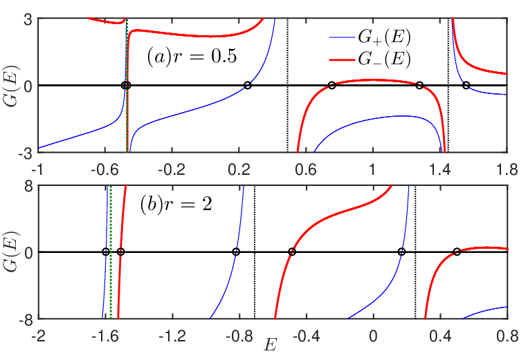
The zeros of this -function can give the regular spectrum. The eigenfunction is then obtained through Eq. (4) with the eigenenergy. To demonstrate this point, we plot the -function for and in Fig. 1. The zeros reproduce all regular spectra, which can be confirmed by the numerical exact diagonalizations in the truncated Fock space. The spectra for a few typical values of and are displayed in Fig. 2.

III First-order QPTs
The level crossings in the QRM and its variants are ubiquitous as long as the parity is conserved. But the level crossings of the ground-state and the first-excited state energy does not always exist. This special level crossing is just a criterion of the first-order quantum phase transition, because the first derivative of the ground-state energy with respect to the coupling constant is discontinuous.
In the two-level atom and the cavity coupling systems, the well-defined pole structure of the derived transcendental functions are very useful. To the best of our knowledge, the characteristics of these poles can be used to analyze the level distribution Braak, level crossings Zhong, and spectra collapse Chen2012; duan. These subtle issues are however hardly settled by the numerics as well as the analytical treatments without poles. We will use the first pole to locate the level crossing points of the ground-state and the first-excited state in the following.
To show the level crossings in the present ARSM in general, we also analyze the pole structure of the derived G-function (5). The vanishing coefficient of in Eq. (35) yields the -th () pole of the G-functions
| (6) |
If the right-hand-side of Eq. (35) is also zero, we can then obtain the values of and at crossing point above the first pole if , and are given. All crossing points above the first pole line shown in Fig. 2 are consistent with the analytical predictions.
In particular, because of in the present scheme, the first pole is however given by the vanishing denominator of in Eq. (34) for
| (7) |
which is not included in the general poles described in Eq. (6). This first pole equation is exactly reduced to that in the isotropic RSM Xie if setting , and the anisotropic QRM Fanheng if .
The poles given in Eqs. (7) and (6) are also exhibited in Fig. 1 with dotted lines. The G-curves at these poles indeed show the diverging behavior. As usual, if both and in G-function (5) are analytic at these pole energies, one obtains the Juddian solutions for doubly degenerate states Judd. In this case, two adjacent energy levels with the even and odd parity can simultaneously intersect with the associated pole line , in the energy spectra. Below we focus on the possible level crossing of the first two lowest levels associated with the first pole () in this model, and skip the discussions on the whole Juddian solutions, which are in fact similar to the previous ones in both the isotropic QRM Braak and the anisotropic QRM Fanheng.
At the first pole energy , the denominator of is zero, so is analytic only if its numerator in Eq. (34) vanishes, yielding a special coupling strength where the ground-state energy and the first-excited state energy cross, i. e. the critical point of the first-order QPT
| (8) |
It can be reduced to that in the anisotropic QRM if setting Fanheng, and in the isotropic RSM if Xie. The critical points given by Eq. (8) are demonstrated in Fig. 2 (a), (b), and (d) with open circles. The absence of the first-order QPT in Fig. 2 (c) is due to the fact that no real solution exists in Eq. (8) at those parameters. Especially in Fig. 2(d), the two lowest levels are too close to be discerned after the crossing point. Fortunately, it can be detected by the present analytical study.
One can find that in the present ARSM, the first-order QPT can be induced by the presence of either the anisotropy or the nonlinear Stark coupling on the condition that . The first-order QPT is still possible in this model even for , which is however forbidden in the anisotropic QRM. In addition, the first-order QPT can also occurs when if , however it is impossible in the isotropic RSM for Xie. The parameter range for the occurrence of the first-order QPT in the present model is much more broader than the previous ones.
The first-order phase transition occurs at finite model parameters only if the Juddian solution associated with the first pole (7) exists. In the isotropic QRM (), the first Juddian solution () is absent Braak. Only if and/or , such a Juddian solution would appear. For special values of the model parameters, the first pole can be lifted because both the numerator and the denominator of vanishes. Thus in this case, the eigenvalues therefore have no definite parity, and a double degeneracy of the eigenvalues occurs.
As found in Ref. Xie, the first crossing energy is in the isotropic RSM. If is absent, the crossing energy is negatively infinite, which cannot be reached by the first two levels, consistent with the absence of the first-order QPT in the isotropic QRM. But for finite , the crossing energy becomes finite, so it is possible that the first two levels cross somewhere at this energy. This possibility is just induced by the the Stark coupling. For the anisotropic QRM, in the extremely case, e.g. RWA, there is always an eigenenergy , the adjacent energy level must cross this energy as the coupling strength increases. With the addition of the counter rotating-wave terms, as long as its coupling strength is weaker than that of the rotating-wave term (i.e., ), the level crossing of the first two levels must happen Fanheng. The first-order QPT however disappears if , which obviously can be attributed to the competition between the rotating and counter-rotating interaction terms. In the present more complicated ARSM, both the Stark coupling and the anisotropy cooperate to enlarge the parameter range of the first-order QPT, as demonstrated above. In short, the first-order QPT depends on the interplay among the Stark coupling, the rotating-wave coupling, and the counter-rotating wave coupling.
IV Continuous quantum phase transitions at
It is known that the continuous QPT would occur in the QRM in the infinite frequencies ratio plenio, which should also happen in the present ARSM. In this section, we do not discuss this obvious continuous QPT, but explore the continuous QPT in the ARSM at finite frequencies ratio for the special Stark coupling .
Note that the solution at cannot be given in the above BOA, but can be obtained in another way as described in Ref. Xie. To this end, we may write the ARSM Hamiltonian in the basis of
| (9) | |||||
Comparing with the Hamiltonian (1), we have , where . If , i.e., the isotopic RSM is recovered, while if , i.e., , it corresponds to the RSM in the RWA.
We can map the ARSM Hamiltonian at to an effective quantum oscillator, the details are given in Appendix B. The solutions to the eigenenergies are given by solving Eq. (40) self-consistently. Obviously, the whole energy spectra separates into two branches: the upper one and the lower one . The real lower spectra only exist before the critical coupling
| (10) |
and the upper bound of the low spectra is .
For , all results can be straightforwardly obtained by replacing and by and , respectively. The corresponding critical coupling strength
| (11) |
and the upper bound of the lower energy spectra is .

Figure 3 presents several low energy levels in the lower spectra with different parameters. To show more clear, the energy is shifted by the corresponding upper bound of the low energy spectra. All levels close at the critical points given by Eq. (10) for or Eq. (11) for .
Energy gap: The low energy spectra equation (40) for can be rewritten as
| (12) |
where and . Below we omit the superscript in and for simplicity. When , . Note that the right-hand side of Eq. (12) is finite in this limit, the first term of the left-hand side reveals that must be of the following form:
| (13) |
or else the left-hand-side is infinite. So the energy gap between the ground state (n=0) and the first excited state (n=1) is
| (14) |
This is to say that, at , the energy gap closes at with a critical exponent . Generally, in the continuous QPT, the energy gap displays a universal scaling behavior, , where is the (dynamics) critical exponent Sachdev. This gap exponent can be confirmed by solving Eq. (40) self-consistently, as shown in the left plot of Fig. 4.
If , the counter-rotating wave coupling is absent, this is just the RWA, and Eq. (12) then becomes
| (15) |
In this case, must be of the form
| (16) |
so the energy gap is
| (17) |
with the gap exponent , which is also verified in the right plot of Fig. 4.

Very interestingly, the real solution for the eigenenergy can even exist above in the RWA, in sharp contrast to any case. Equation (40) at gives
| (18) |
where denotes the upper (lower) spectra. The extension to the is straightforward, and will not be presented here.
The derivative of the energy level with respect to in the lower spectra is given by
| (19) |
the extremal condition happens exactly at the critical coupling by Eq. (10) with
It is obvious that, for , the low energy spectra increase with , while for , the low energy spectra decrease with . Thus the ground-state energy corresponds to for . However, for , the ground-state energy is surprisingly corresponding to the infinite ,
| (20) |
So the gap between the first-excited state and ground state always vanishes for , because
It just demonstrates the appearance of photonic Goldstone modes above a critical point. In the Dicke model with infinite two-level atoms in the RWA, a Goldstone soft mode appears above a critical point as a consequence of the symmetry breaking Ciuti. Here although the RWA is also made, only one two-level atom is involved. In the ARSM under the RWA, the system also possesses symmetry, and is broken above the critical points.
In the ground state of the RSM under the RWA, the photonic number below , but above , suggesting a special superradiant phase.
V Conclusion
In this work, we find that both the first-order and the continuous QPTs are present in the ARSM where both the nonlinear Stark coupling and the anisotropic dipole linear coupling are present. Among the previous QRM and the Dicke model, as well as their generalized models, both types of QPTs have not been observed in the same model in the literature.
The first-order QPT is detected analytically by the pole structure of G-functions based on the BOA. The critical coupling strength of the phase transitions is obtained analytically, which is determined by both anisotropy and the nonlinear Stark coupling. On the other hand, the continuous QPT is also found in this model at the special values of the Stark coupling strength for the closing energy spectra at the critical points. The energy gap follows an universal power-law scaling ansatz in any ARSMs. The energy-gap exponent for , i.e., the RWA; while for , indicating that the presence of any counter-rotating wave terms would change the universality class of this model. In the RWA, since the gap is always closed above the critical points, one phase having Goldstone mode gapless excitations then appears.
The continuous QPT undergoes in the QRM at the infinite frequency ratio, occurs in the Dicke model in the thermodynamic limit. These prerequisite conditions are however not required in the present ARSM for the occurrence of the QPTs. Especially in the RWA, the critical coupling can be weak sufficiently by tuning the qubit frequency in the ARSM. We therefore believe that the continuous QPTs might be easily demonstrated experimentally or in quantum simulations based on some solid-state devices, such as the cavity (circuit) QEDs and the ion-trap, where the ARSM Hamiltonian can be realized.
ACKNOWLEDGEMENTS We acknowledge useful discussions with Lei Cong. This work is supported by the National Science Foundation of China (Nos. 11674285, 11834005), the National Key Research and Development Program of China (No. 2017YFA0303002),
∗ Email:qhchen@zju.edu.cn
Appendix A Derivation of G-function of the ARSM by BOA
In this Appendix, we derive a transcendant function to the ARSM by BOA. By using the transformation (2) we obtain the transformed Hamiltonian in the matrix form
| (21) |
where and. It can be expressed in terms of new operator defined in Eq. (3) with the four matrix elements below
In terms of the eigenfunction (4), we can obtain the Schrödinger equations for both upper and lower levels, then projecting both sides of the Schrödinger equations onto gives
| (22) | |||||
| (23) | |||||
where
Multiplying the Eq. (22) by and Eq. (23) by , we have
| (24) | |||||
| (25) | |||||
Summation of Eq. (24) and Eq. (25) gives
| (32) | |||||
To remove the term containing , the displacement should be
| (33) |
Then by Eq. (32) we have
| (34) |
Inserting Eq. (34) to Eq. (22) at gives
| (35) |
where
Starting from , then can be obtained by Eq. (34) at and by Eq. (35). By a similar procedure, we can obtain any th coefficients and .
Alternatively, the eigenfunction can also be expanded in the another Bogoliubov operator with the opposite displacement as
| (36) |
due to the parity symmetry. Here is defined in the similar way as .
Assuming both wavefunctions (4) and (36) are the true eigenfunction for a nondegenerate eigenstate with eigenvalue , they should be proportional to each other, i.e., , where is a complex constant. Projecting both sides of this identity onto the original vacuum state , we have
where
Eliminating the ratio constant gives
Immediately, we obtain the following well-defined transcendental function, the s-ocalled -function, as
| (37) |
where corresponds to odd(even) parity. Interestingly, this -function can be reduced to those of the RSM if Xie, the anisotropic QRM if Fanheng, and the isotropic QRM if and Braak. It is worth noting that even in the presence of both the nonlinear Stark coupling and the anisotropic linear dipole coupling in this generalized model, the G-function can still be obtained within the BOA in the concise way.
Appendix B Solutions to the Anisotropic Rabi-Stark Model at
In this Appendix, we turn to the ARSM at which solutions cannot be covered in Appendix A.
In terms of the position and momentum representations, , Hamiltonian (9) at can be written as
| (38) |
For the eigenfunction , the Schrödinger equations for the upper and lower level now are
where is the eigenvalue. Inserting to the first equation results in the effective one-body Hamiltonian for
where
| (39) |
which is just a quantum harmonic oscillator with an effective oscillator frequency
So the eigenenergy is then expressed as
| (40) | |||||
Solving this equation self-consistently would give solutions to the ARSM at .
References
- (1) I. I. Rabi, Phys. Rev. 51, 652 (1937).
- (2) D. Braak, Q.-H. Chen, M. Batchelor, and E. Solano, J. Phys. A: Math. Gen. 49, 300301 (2016).
- (3) E. T. Jaynes, and F. W. Cummings, Proc.IEEE 51, 89 (1963).
- (4) M. O. Scully, and M. S. Zubairy, Quantum Optics (Cambridge University Press, Cambridge, 1997); M. Orszag, Quantum Optics Including Noise Reduction,Trapped Ions, Quantum Trajectories, and Decoherence(Springer, Berlin, 2007), 2nd ed.
- (5) T. Niemczyk, F. Deppe, H. Huebl, E. P. Menzel, F. Hocke, M. J. Schwarz, J. J. Garcia-Ripoll, D. Zueco, T. Humer, E. Solano, A. Marx A , and R. Gross, Nat. Phys. 6, 772 (2010).
- (6) P. Forn-D Píaz, J. Lisenfeld, D. Marcos, J. J. Garca-Ripoll, E. Solano, C. J. P. M. Harmans, and J. E. Mooij, Phys. Rev. Lett. 105, 237001 (2010).
- (7) D. Leibfried, R. Blatt, C. Monroe, and D. Wineland, Rev. Mod. Phys. 75, 281 (2003).
- (8) J. Clarke and F. K. Wilhelm, Nature 453, 1031 (2008).
- (9) F. Yoshihara, T. Fuse, S. Ashhab, K. Kakuyanagi, S. Saito, and K. Semba, Nat. Phys. 13, 44 (2016).
- (10) P. Forn-Díaz, J. J. García-Ripoll, B. Peropadre, J.-L. Orgiazzi, M. A. Yurtalan, R. Belyansky, C. M. Wilson, and A. Lupascu, Nat. Phys. 13, 39 (2016).
- (11) J. Casanova, G. Romero, I. Lizuain, J. J. García-Ripoll and E. Solano, Phys. Rev. Lett. 105, 263603 (2010).
- (12) D. Braak, Phys. Rev. Lett. 107, 100401 (2011).
- (13) Q.-H. Chen, C. Wang, S. He, T. Liu, and K. L. Wang, Phys. Rev. A 86, 023822 (2012).
- (14) S. He , C. Wang, Q.-H. Chen, X. Z. Ren, T. Liu, and K. L. Wang, Phys. Rev. A 86, 033837 (2012); S. He, Y. Zhao, and Q-H. Chen, Phys. Rev. A 90, 053848 (2014).
- (15) H.-H. Zhong, Q.-T. Xie, M. T. Batchelor, and C.-H. Lee , J. Phys. A 46, 415302 (2013); J. Phys. A 47, 045301 (2014).
- (16) Q.-H. Chen, T. Liu, Y. Y. Zhang, and K-L. Wang Europhys. Lett. 96, 14003 (2011).
- (17) C. J. Gan and H. Zheng, Eur. Phys. J. D 59, 473 (2010).
- (18) Z.-J. Ying, M. X. Liu, H.-G. Luo, H.-Q. Lin, J. Q. You, Phys. Rev. A 92, 053823 (2015).
- (19) M.-J. Hwang, R. Puebla, and M. B. Plenio, Phys. Rev. Lett.115, 180404 (2015).
- (20) M. X. Liu, S. Chesi, Z.-J. Ying, X. S. Chen, H.-G. Luo, H.-Q. Lin, Phys. Rev. Lett. 119, 220601 (2017).
- (21) P. Forn-Díaz, L. Lamata, E. Rico, J. Kono, E. Solano Rev. Mod. Phys. 91, 025005 (2019).
- (22) A.F. Kockum, A. Miranowicz, S. De Liberato, S. Savasta, F. Nori, Nat. Rev. Phys. 1, 19(2019).
- (23) A. Le Boité, arXiv:2001.08715.
- (24) Y. X. Yu, J. Ye, and W. M. Liu, Scientific Reports 3, 3476 (2013).
- (25) Q. T. Xie, S. Cui, J. P. Cao, L. Amico, and H. Fan, Phys. Rev. X 4, 021046 (2014).
- (26) M. Tomka, O. E. Araby, M. Pletyukhov, and V. Gritsev, Phys. Rev. A90, 063839 (2014).
- (27) S. I. Erlingsson, J. C. Egues, and D. Loss, Phys. Rev. B 82, 155456 (2010).
- (28) M. Schiroa, M. Bordyuh, B. Otu ztop, and H. E. Tureci, Phys. Rev. Lett. 109, 053601 (2012).
- (29) A. Wallraff, D. I. Schuster, A. Blais, L. Frunzio, R. S. Huang, F. Majer, S. Kumar, S. M. Girvin, and R. J. Schoelkopf Nature (London) 159, 162 (2004).
- (30) C. Zhu, L. Dong, and H. Pu, Phys. Rev. A 94, 053621 (2016).
- (31) A. L. Grimsmo, and S. Parkins, Phys. Rev. A 87, 033814 (2013).
- (32) A. L. Grimsmo, and S. Parkins, Phys. Rev. A 89, 033802 (2014).
- (33) H.-P. Eckle and H. Johannesson, J. Phys. A: Math. Theor. 50, 294004 (2017).
- (34) A. J. Maciejewski, M. Przybylska, and T. Stachowiak Phys. Lett. A 379 1505 (2015).
- (35) Y-F. Xie, L. W. Duan, and Q.-H. Chen, J. Phys. A: Math. Theor. 52, 245304 (2019).
- (36) Y-F. Xie, and Q.-H. Chen, Commun. Theor. Phys. 71, 623 (2019).
- (37) L. Cong, S. Felicetti, J. Casanova, L. Lamata, E. Solano, and I. Arrazola, Phys. Rev. A 101, 032350 (2020).
- (38) Z. Q. Zhang, C. H. Lee, R. Kumar, K.J. Arnold, S. J. Masson, A. L. Grimsmo, A. S. Parkins, and M. D. Barrett, Phys. Rev. A 97, 043858 (2018).
- (39) L. W. Duan, S. He, D. Braak, Q.-H. Chen, EPL, 112, 34003(2015); L. W. Duan, Y.-F. Xie, D. Braak, Q.-H. Chen, J. Phys. A: Math. Theor. 49, 464002 (2016).
- (40) B. R. Judd, J. Phys. C 12, 1685 (1979).
- (41) A. Baksic and C. Ciuti, Phys. Rev. Lett. 112, 173601 (2014).
- (42) S. Sachdev, Quantum Phase Transitions, 2nd ed. (Cambridge University Press, Cambridge, England, 2011).