The Classical Symmetron Force in Casimir Experiments
Abstract
The symmetron is a typical example of screened modified gravity, wherein the symmetron force is dynamically suppressed in dense environments. This allows it to hide in traditional tests of gravity. However, the past decade has seen great experimental progress towards measuring screened forces in the laboratory or in space. Screening relies on nonlinearities in the equation of motion, which significantly complicates the theoretical analysis of such forces. Here, we present a calculation of the symmetron force between a dense plate and sphere surrounded by vacuum. This is done via semi-analytical approaches in two limiting cases, based on the size of the sphere: large spheres are analyzed via the proximity force approximation, whilst small spheres are treated as screened test particles. In the intermediate regime we solve the problem numerically. Our results allow us to make contact with Casimir force experiments, which often employ a plate and sphere configuration for practical reasons, and may therefore be used to constrain symmetrons. We use our results to forecast constraints on the symmetron’s parameters for a hypothetical Casimir experiment that is based on the current state of the art. The forecasts compare favorably to other leading laboratory tests of gravity, particularly atom interferometry and bouncing neutrons. We thus conclude that near-future Casimir experiments will be capable of placing tight new bounds on symmetrons. Our results for the symmetron force are derived in a scale-invariant way, such that although we here focus on Casimir experiments, they may be applied to any other plate-sphere system, ranging from microscopic to astrophysical scales.
I Introduction
The accelerated expansion of the Universe has motivated new classes of scalar-tensor theories Khoury 2010; Brax 2018 that go beyond general relativity (GR) Einstein 1916. As the coupling of the scalar sector to matter is generically not explicitly forbidden by the symmetries of these scalar-tensor theories, there is in general no theoretical restriction on the existence of scalar “fifth forces” between matter particles. On the other hand, such forces are experimentally tightly constrained in the Solar System and by laboratory experiments Will 1993; Burrage and Sakstein 2018; Brax et al. 2018a. Compatibility with these bounds then requires the fifth force to be either tuned to be extremely weak, or to be dynamically suppressed in certain situations.
This latter approach, dubbed as “screening”, has generated a great deal of interest over the past two decades Brax 2013. There are four main classes of screening mechanisms that have been discovered so far (see Joyce et al. 2015 for a comprehensive review):
- 1.
chameleons Khoury and Weltman 2004: The scalar field becomes heavy, and therefore short-ranged, in dense environments.
- 2.
Damour-Polyakov Damour and Polyakov 1994: The scalar field decouples when the coupling to matter is dynamically driven to zero. Examples are given by the symmetron Pietroni 2005; Olive and Pospelov 2008; Hinterbichler and Khoury 2010; Hinterbichler et al. 2011 and the dilaton in the large string coupling limit Brax et al. 2010a.
- 3.
K-mouflage: The steep field gradients of the scalar field help to suppress fifth forces Babichev et al. 2009; Brax et al. 2013; Brax and Valageas 2014.
- 4.
Vainshtein: Fifth forces are suppressed in regions where the second derivatives of the scalar field are sufficiently large Vainshtein 1972; Nicolis et al. 2009.
The phenomenology of the first two mechanisms turns out to be similar, i.e. they both screen fifth forces where the surface Newtonian potential of the body is sufficiently large Brax et al. 2012a. For concreteness, in this paper we focus on symmetrons, even though extension to other scenarios, particularly chameleons, is possible.
Symmetron gravity has been extensively studied in contexts ranging from cosmological large-scale structure to laboratory experiments. As mentioned above, the main observable effect of symmetrons is that matter feels an extra force compared to the general relativistic gravitational interaction. Hence the large-scale dark matter distribution in the Universe is affected and differs from the GR case. Such changes are investigated in Refs. Davis et al. 2012a; Brax et al. 2012b. On smaller scales, symmetrons are naturally expected to alter the collapse dynamics of dark matter shells, and, as such, leave observable imprints on the density profiles of dark matter halos Contigiani et al. 2019, as well as to alter the halo mass function Taddei et al. 2014. Moreover, symmetron fifth forces will necessarily alter the velocity dispersion of dark matter tracers in halos, therefore leading to a potential mismatch between the dynamical halo mass and the lensing mass. This feature is exploited as a test of symmetron gravity in Ref. Clampitt et al. 2012. Another interesting class of tests is suggested at galactic and stellar scales. Particularly, the effects on stellar dynamics in galaxies and globular clusters are explored in Refs. OHare and Burrage 2018; Llinares 2018. Refs. Brax et al. 2014; Zhang et al. 2017 consider changes in energy output from binary pulsars, Ref. Davis et al. 2012b investigates the effect of screening on stellar evolution and Ref. Jain et al. 2013 studies changes in stellar physics induced by the symmetron force. The presence of a scalar force is also expected to induce a mismatch between the stellar and gas components in galaxies. This idea in the context of symmetron gravity is explored in Ref. Desmond et al. 2018.
Besides cosmological and astrophysical tests, symmetrons can also be tested in laboratory experiments. Notably, atom interferometry experiments have been able to constrain them significantly Burrage et al. 2016; Jaffe et al. 2017; Sabulsky et al. 2019. These are complemented by torsion balance experiments Upadhye 2013; Brax and Davis 2015. Constraints also follow from quantum effects of the symmetron which affect the anomalous magnetic moment of the electron Brax et al. 2018b and lead to corrections to the energy levels of neutrons in the gravitational field of the Earth Cronenberg et al. 2018.
In this paper, we focus on new bounds on symmetrons that may be obtained from Casimir force sensors Lamoreaux 1997; Decca et al. 2005a; Decca et al. 2003. Although conceived as detectors for the quantum mechanical Casimir-Polder force, these systems are also sensitive to any additional forces Decca et al. 2005b; Decca et al. 2003, including classical screened fifth forces Brax et al. 2007. The advantage of using Casimir force sensors to look for new forces is that they probe very short distance scales ( m) and therefore larger particle masses compared to longer-range fifth force detectors in the laboratory or the Solar System (see, for instance, Ref. Berge et al. 2018). Casimir experiments have been used to constrain chameleons Brax et al. 2007, and new experiments Brax et al. 2010b will provide results soon Almasi et al. 2015; Sedmik and Brax 2018. However, such constraints have not yet been presented for symmetrons, mainly due to a lack of theoretical calculations of the symmetron force between extended objects Burrage and Sakstein 2018.
In this article we address this shortcoming by computing the symmetron force between a plate and a sphere. We focus on this case for two reasons. First, it is perhaps the simplest asymmetric geometry with two extended objects that one could consider. Second, our results will be directly applicable to realistic Casimir force sensors, which often use a plate and a sphere for practical experimental reasons Chen et al. 2016, rather than two parallel plates (as in some previous experiments such as CANNEX Almasi et al. 2015). This configuration leads to significant theoretical challenges, as screened fifth forces generically have nonlinear equations of motion which are difficult or impossible to solve in less symmetric setups. In this paper we overcome this hurdle by identifying two limiting regimes that allow the symmetron force between a sphere and a plate to be approximated analytically. We also present numerical solutions that interpolate between the limiting cases, and which verify our analytic treatments.
We do this by splitting our analysis into three regions, determined by the size of the dimensionless quantity , where is the radius of the sphere and is approximately the mass of the symmetron in vacuum. Physically, this measures the radius of the sphere in units of the symmetron’s Compton wavelength. Our three regions are thus and . In the first and third regions we are able to exploit the hierarchy of scales between the sphere radius and the symmetron Compton wavelength to obtain accurate analytic approximations to the force. In the middle region we solve the problem numerically. It is fortunate that the numerical solution is easiest to obtain when all scales in the problem are comparable, given that this is precisely the regime in which analytic approximations break down. Our results cover several orders of magnitude in sphere radii and separations, and our methodology can be applied to more extreme configurations, not directly reported in this paper. Hence we present a complete solution for the symmetron force in the plate-sphere system. Furthermore, the solutions we obtain are fully nonlinear; at no point is the theory linearized about the background vacuum expectation value (apart from the derivation of the screening factor of a dense sphere, which is standard). We then apply our solutions to a realistic Casimir sensor, and show that the results from future measurements will be able to constrain a large part of the symmetron’s parameter space. Although our results are applied to a specific type of problem, i.e. the force between a sphere and a plate which are of laboratory sizes, we emphasize that these solutions are scale-independent and could apply to many other setups such as astrophysical problems.
In this paper we concentrate on the classical symmetron interaction between a sphere and a plate. We do not take into account quantum effects which can be significant. Such quantum effects have been studied in Ref. Brax and Fichet 2019 for the plate-plate case, and as a rule, the effects dominate when the scalar field between interacting bodies can be considered almost massless and the self-interaction of the scalar field is large. The forecasts we present here are in the small self-interaction regime, where we expect the quantum effects to be negligible. We leave a comprehensive analysis of the quantum interactions in the plate-sphere system for future work.
This paper is organized as follows. We first review the symmetron screening mechanism in Sec. II. In Sec. II.2, we focus on the two-parallel-plate case. This provides us with intuition for how analytic approximations should be made for the plate-sphere configuration, and additionally, allows us to validate our numerical setup. In Sec. III, we analyze the plate-sphere system analytically, and provide analytic approximations for the two cases of large and small spheres. In Sec. IV, we discuss our procedure for numerically integrating the symmetron equation of motion and computing the force between the sphere and the plate in regimes that are not captured by our analytic results. We show that in the regions of the parameter space where we expect both analytic and numerical approaches to be valid, the results are in very good agreement. We test our numerical framework for a range of configuration parameters and show that it can be applied to any experimental setup. In Sec. V, we propose a Casimir force experiment, based on a plate-sphere configuration and with specifications and sensitivity that closely follow those of existing state-of-the-art experiments. We place forecast constraints on the symmetron’s free parameters using the expected Casimir bounds on fifth forces. We compare our constraints to those obtained from other laboratory experiments based on atom interferometry Jaffe et al. 2017, torsion balances Upadhye 2013, and ultracold bouncing neutron measurements Cronenberg et al. 2018. Finally, we conclude in Sec. VI.
II The symmetron model
II.1 The model
The symmetron is a real scalar field with a Lagrangian density11 1 We are using units where and are working with the mostly-plus metric convention. given by
| (1) |
Notice the quadratic coupling of the symmetron field to the ambient matter density , which leads to a symmetry-breaking effective potential,
| (2) |
In the absence of matter, and the effective potential has minima at with . In this case the effective potential reduces to that of a Higgs-like field. Without loss of generality we will consider the positive vacuum value only. The breaking of the symmetry can lead to domain walls Burrage et al. 2016; Llinares and Brax 2019, which are not expected to be present in the experimental settings that we consider. When the ambient matter density is above the critical value , the minimum of the effective potential is located at . If is independent of time then the equation of motion for static field configurations is an elliptic partial differential equation given by
| (3) |
The quadratic coupling to matter also leads to a symmetron force experienced by a test particle with mass , given by
| (4) |
Notice that the force is proportional to the symmetron’s local field value—in media with density greater than the critical density, , the ambient field value is driven to and the symmetron force switches off. Another remarkable property of the symmetron is that extended objects can be screened, that is, the symmetron force may not be proportional to the total mass of the object. We review this phenomenon here, for the case of a finite-sized sphere of density . This treatment closely follows that of Ref. Hinterbichler and Khoury 2010.
We compute the symmetron force between a sphere with mass and a test particle with mass . We first compute the symmetron field profile around the sphere, and then compute the force on the test particle with Eq. (4). The sphere is taken to have radius and density , where is a constant and is the Heaviside step function. We assume that the sphere is dense enough to restore the symmetry, i.e. . Otherwise, the sphere is not capable of perturbing the symmetron field away from the vacuum expectation value (VEV) and the symmetron force is negligible.
First we solve the equation of motion inside the sphere. Deep inside the sphere we expect to approach the minimum of the effective potential in the symmetric phase. We can therefore approximate the effective potential by a quadratic function located at , and find
| (5) |
where we have introduced . Note that we have set one of the boundary conditions such that does not diverge at the origin. We are left with a normalization factor , which will be determined later. Next we solve for the field outside the sphere. We demand that the field minimizes its potential far away from the sphere: as . This time, we linearize the equation of motion about and find
| (6) |
where we have an undetermined constant of integration . To fix the constants and , we impose that the field and its first derivative match at the surface of the sphere . We are ultimately interested in the symmetron force exerted on the test particle, so we will only need the constant , for which we find
| (7) |
For the symmetron screening mechanism to work we must assume that the sphere is much denser than the symmetron critical density, i.e. . Taking this limit, the coefficient becomes
| (8) |
where we have defined the dimensionless parameter for convenience.
Let us now consider a fixed matter coupling , and study the limiting cases of a very small and light sphere versus a very large and dense sphere. In the first limit , and we have
| (9) |
The external field is therefore given by
| (10) |
The (attractive) symmetron force exerted on a test particle follows from Eq. (4), and to leading order in reads
| (11) |
Evidently small, light particles couple to each other with a symmetron force proportional to the product of their masses and inversely proportional to the square of the distance between them, exactly as they do in GR. The relative strength of their interaction, compared to Newtonian gravity, is
| (12) |
where is the Planck mass.
Let us now consider the limit of a dense and large sphere, i.e. . The integration constant in the external field becomes
| (13) |
This time, the symmetron force experienced by the test particle is
| (14) |
where we have defined a screening factor for the sphere as
| (15) |
Notice that the symmetron force is no longer proportional to the total mass of the sphere, but only to a minuscule fraction of the sphere’s total mass. The force is thus sharply suppressed compared to what one might have guessed based on Eq. (11) alone. This phenomenon is the essence of screening.
More generally, the symmetron force between two spheres involves a screening factor for each sphere. Combining Eqs. (11) and (14), we have
| (16) |
as long as the two spheres can be considered as mutual test objects, i.e. not disturbing the field profile generated by one another, where the screening factors are
| (17) |
with . The screening factor will play a crucial role in describing the behavior of a small but very dense sphere in the next section.
II.2 The symmetron force between parallel plates
Let us now discuss another simple density configuration, namely, two infinitely dense parallel plates separated by a distance , and analyze the field profile and the resulting force between the plates; see Fig. 1. As the density of plates is taken to be infinite, the symmetron field can be taken to be zero inside the plates. Additionally, the exterior solution is unaffected by the separation of the plates, hence we are interested only in the dynamics of the field between the plates.
The parallel-plates configuration is important for two main reasons. First of all, thanks to the planar symmetry of the configuration the symmetron equations of motion can be analytically integrated and the corresponding fifth force can be calculated exactly. This will allow us later to verify the accuracy of our numerical integrator of the symmetron equation of motion, as well as our procedure of numerical force calculation. Besides this technical aspect, as we will see later, the parallel-plates setup can give important insights into the field configuration and the force in the plate-sphere setup.

II.2.1 Simple approximate treatment
We start our discussion with an approximate, qualitative treatment of this system. When the separation between the plates is large, , the field has sufficient room to roll to the vacuum expectation value. The relevant length scale over which the symmetron field is able to vary significantly is the Compton wavelength in vacuum, . The gradient energy per unit area of the plate can then be approximated as
| (18) |
where is the surface area of one of the plates. Note that due to our convention in Eq. (2) the true vacuum has a zero potential energy. As a result the energy of the field configuration for can be approximated as
| (19) |
up to an constant. This indicates that the energy stored in the symmetron field does not depend on the plate separation , hence the force between the plates, determined through , is zero: .
When the separation is sufficiently small, , the field would have to spend a significant amount of gradient energy in order to achieve the true vacuum. As a consequence, the lowest energy configuration is the one in which the field stays in the false vacuum, so everywhere between the two plates. In this case there is no gradient energy, and the total energy per unit plate area is
| (20) |
The force per unit area is, therefore, .
In summary, according to our qualitative analysis the force between the two plates behaves as
| (21) |
where is a crossover separation below which the field is zero everywhere between the plates. According to the qualitative analysis above we are only able to estimate the order of magnitude of the crossover separation to be . In the next subsection we will be able to determine its exact value.
Given these estimates we can now discuss the influence of the quantum corrections to the classical force Brax and Fichet 2019. The quantum interaction between the two plates is not suppressed when the scalar field can be considered as massless in vacuum, i.e. when . In this case the two plates attract each other with a quantum pressure
| (22) |
which is one half of the electromagnetic result as the scalar has only one polarization. In this regime, the classical interaction dominates when
| (23) |
which can be safely taken to be in the range . In the following, we will always assume that the self-coupling of the symmetron is small enough to neglect the quantum interaction.
II.2.2 Improved pressure between plates
The treatment presented above gives a simple estimate of the force. However, an exact solution is also possible. As previously mentioned, the symmetries of this density configuration allow the field profile to be found exactly in terms of special functions. Particularly, the solution for the field in the intervening region between the plates is found to be
| (24) |
where is the Jacobi elliptic function; see, for instance, Refs. Brax and Pitschmann 2018; Burrage et al. 2019 for a complete treatment. The parameter ranges between and and is fixed by the boundary condition that the field must vanish at the surface of each plate, . This leads to the condition
| (25) |
Note that is the value of the field in the middle of the intervening region, normalized by the VEV , i.e. . It is not possible to isolate analytically, although we can note the following:
- •
If , we must have ; see Refs. Upadhye 2013; Brax and Davis 2015 for further explanation.
- •
As , .
- •
When , by continuity we can expect . We can then Taylor expand Eq. (25) and obtain , which we must stop trusting as soon as is sufficiently larger than .
Outside the intervening region, the field rises monotonically towards the VEV,
| (26) |
where is the width of the plate.
We can compute the scalar force on an extended object in the following way Hui et al. 2009. The -momentum in a volume of space is given by
| (27) |
where is the total energy-momentum tensor for both the matter and scalar fields, . We choose to be large enough so that it encompasses the entire extended object, but small enough that the matter fields dominate the integral. This ensures that the momentum of the volume is a good approximation of the momentum of the extended object itself. The force is the time derivative of the momentum, so we have
| (28) |
where we have used the conservation of the energy-momentum tensor to go from the first integral to the second, and then changed the volume integral over to a surface integral over the outer boundary of the volume with an area element . The matter part of vanishes on the boundary, so we need to integrate only the energy-momentum tensor of the scalar field. Taking into account the symmetries of the problem, we choose to be a rectangular parallelepiped as shown in Fig. 1, the two sides of which are located at small distances from the two surfaces of the plate. The energy-momentum tensor of the scalar field is
| (29) |
and can be computed at any arbitrary point. Obviously, given the symmetries of the configuration, the only non-vanishing component of the force is the -component, which can be written as
| (30) |
using the middle integral in Eq. (28).
Since the scalar field vanishes on the surface of the plate, we obtain
| (31) |
where a prime denotes a derivative with respect to . Note that the right-hand side of this equation is equal to the difference between the boundary values of the stress-energy tensor, as expected from the last expression in Eq. (28). We now use the solutions of the field given by Eqs. (24) and (26), as well as the identities
| (32) |
to calculate the force between the plates. We obtain a force per area
| (33) |
When the distance between the two plates is small, , then and , as we obtained in our qualitative estimation of the force in the previous subsection. When the distance is large, , then and . For general values of , we solve Eq. (25) numerically, using Newton’s method. We plot in Fig. 2 the exact pressure as a function of , as well as the qualitative estimates for small and large distances. Note that the estimated values for small distances, , are in perfect agreement with the exact values, while they are significantly smaller for intermediate distances, ; the estimated and exact values agree for . This is an important observation with implications for calculating the constraints one may want to impose on the symmetron fifth forces using parallel-plates experiments.
III Plate and sphere I: analytic results
In this section, we turn to the problem of computing the classical scalar force between an infinite plate and a finite-radius sphere. The reason for considering this configuration is that Casimir experiments are often built using a plate-sphere system Lamoreaux 1997; Decca et al. 2005a; Chen et al. 2016, as this setup eliminates experimental uncertainty related to proper alignment of two plates.
We assume that the surface of the infinite plate is located at with a sphere of radius facing it, and that the nearest distance between the plate and the sphere is ; see Fig. 3. Although a given experimental setup is likely to have a fixed radius and to probe only a few different separations, our aim in this paper is to compute the symmetron force for any combination of and . This, along with the scale invariance of our solutions, will allow our results to be applicable to any system that resembles a plate-sphere configuration, ranging from microscopic to astrophysical scales. Furthermore, our general approach will enable future work to identify optimal configurations for new Casimir experiments, in order to probe the most interesting regions of the parameter space.
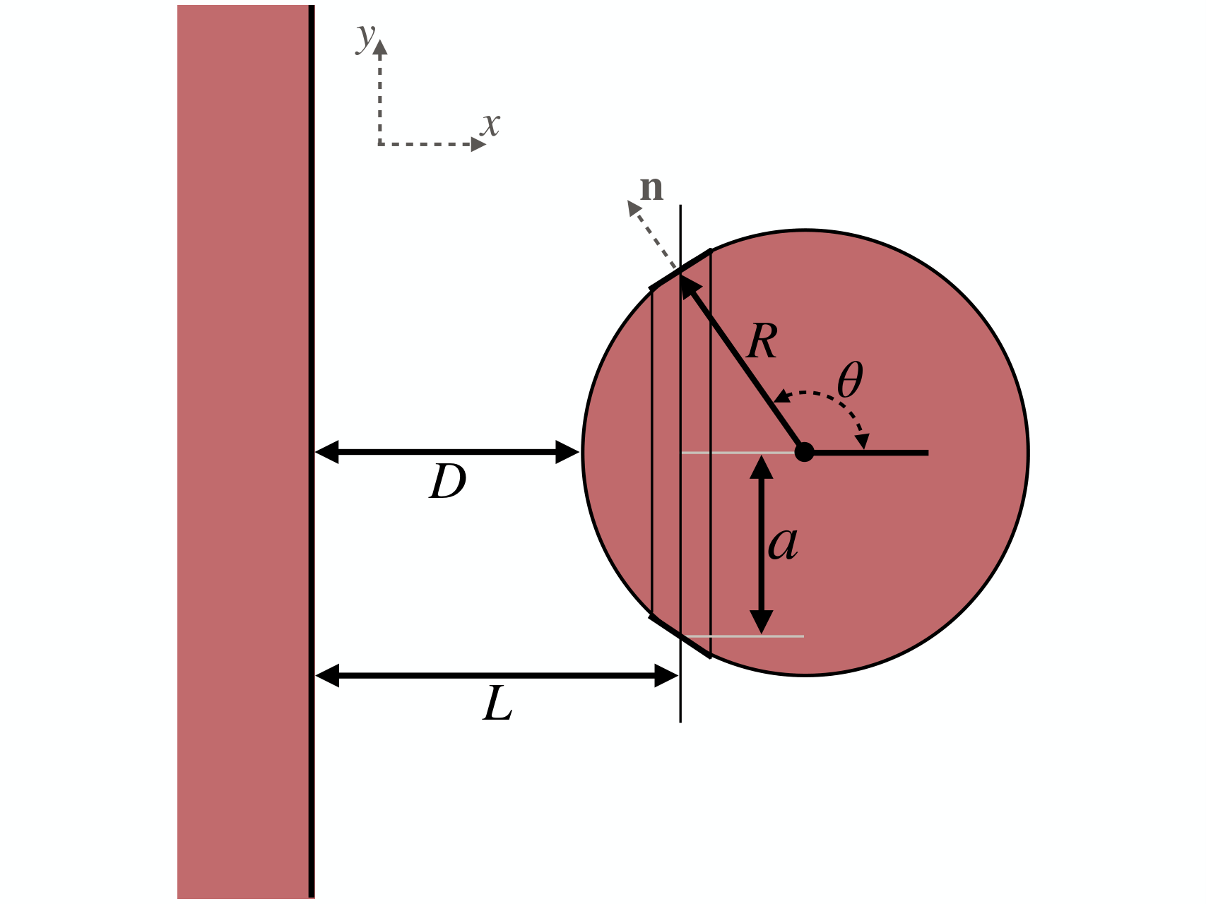
Due to the nonlinearity of the symmetron’s equation of motion, it is impossible to find exact analytic solutions for the field in this configuration. We must therefore work with numerical solutions or analytic approximations in different regimes. In this section, we present approximate solutions for the scalar force in two regimes: (i) large spheres with , and (ii) small spheres with . In the next section, we use numerical solutions to verify these approximations, as well as to provide solutions for of .
III.1 Large sphere
We first analyze the plate-sphere system in the limit that the sphere radius is much larger than the symmetron’s Compton wavelength, i.e. . Our approach is similar to the proximity approximation that is often employed in calculations of the quantum Casimir force between objects with complex geometries; see, for example, Refs. Krause et al. 2007; Brax et al. 2007.
We consider infinitesimally thin ring-like elements of the sphere parallel to the plate, and use the analytic formula for the parallel-plate pressure calculated in the previous section to model the pressure exerted on the element by the plate. Let us consider a ring placed at a distance from the surface of the plate, where is the standard polar angle defined around the -axis (see Fig. 3). The contribution of this ring to the total force experienced by the sphere is approximated as
| (34) |
where is the pressure between two parallel plates separated by the distance , and is the area of the infinitesimal ring element. The factor takes the -component of the force on the ring or corresponds to the cross-sectional area of the sphere directly perpendicular to the plate. The area of the ring is , where is the vertical distance from the infinitesimal ring to the line connecting the plate and center of the sphere.
The total symmetron force exerted on the sphere is then obtained by integrating over the hemisphere nearest the plate and is given by
| (35) |
What remains is to specify the pressure between the parallel plates . In Sec. II.2, we found two different expressions for that. The first one is given in Eq. (21), which is approximate but simple. We will refer to this as . We also found the exact pressure between two plates, given by Eq. (33), which we will refer to as . Although the latter has the advantage of being exact, it does not admit a closed-form solution. Employing the former for now, we note that the pressure is a step function, so only a spherical cap within a distance from the plate contributes to the pressure, and is constant over this area. We therefore compute the attractive force on the spherical cap, which has a height and radius . The cap has cross-sectional area , so the force is
| (36) |
When no part of the sphere is within of the plate, the force is zero:
| (37) |
When all of the near hemisphere is within of the plate, we have
| (38) |
In summary, the force is
| (39) |
We remind the reader that we are working in the regime of large spheres, , so the first case is included only for completeness.
To obtain a more exact result, we could instead have used , given by Eq. (33). In this case, it is not possible to simplify the expression, and we must instead rely on numerical integration. That is, we integrate
| (40) |
where the pressure is given by Eq. (33). A comparison between these two expressions for the symmetron force on a large sphere is given in Fig. 4.
III.2 Small sphere
Let us now calculate the symmetron force between a plate and a small sphere, i.e. . In this limit, we may safely neglect the backreaction of the sphere on the symmetron field profile sourced by the plate alone.22 2 Note that the backreaction, neglected here, may lead to large corrections at very small distances, as explored in Ref. Ogden et al. 2017. This means that the force on the sphere will be proportional to that of a test particle. The constant of proportionality is the screening factor , which is given by Eq. (17). The force on the sphere is therefore
| (41) |
where is the mass of the sphere, and is the field profile generated by the plate alone. Recall that the latter is simply given by
| (42) |
Before putting all these ingredients together let us also recall that we are working in the limit , and as such Eq. (17) indicates that . However, in this limit the mass of the sphere diverges, and as a result the prefactor in Eq. (41) is a non-negligible quantity given by
| (43) |
Putting all these together, Eqs. (42) and (41) give the attractive force
| (44) |
where is the distance from the surface of the plate to the center of the sphere.
The approximate forces we obtained for large and small spheres are plotted in Fig. 4 as functions of the distance between the plate and the sphere. Notice that in the case of the small sphere the force vanishes as the sphere approaches the plate. Intuitively, this may be understood as a consequence of the symmetron’s quadratic coupling to matter: near the plate the ambient field value is driven towards zero, so the coupling between the symmetron and matter becomes weaker and the force is diminished.
IV Plate and sphere II: numerical results
Beyond highly symmetric configurations it is impossible to find exact solutions of Eq. (3). In the previous section, we detailed two useful limiting cases: very large spheres with , and very small spheres with . In these cases it was possible to exploit the hierarchy of scales to make analytic progress.
In this section, we turn to the intermediate regime, where . We are unable to exploit any such hierarchy of scales in this case, so we must resort to numerical integration of the symmetron’s equation of motion. Our results allow us to bridge the gap between the two limiting cases we explored in the previous section. We use a commercial solver,33 3 We used Matlab’s Partial Differential Equation Toolbox, version R2019b, similar to what has been done in Refs. Chiow and Yu 2018; Chiow and Yu 2019. which relies on the finite-element method. For some of the cases, we have checked the solutions using our own numerical code based on the Newton-Gauss-Seidel relaxation algorithm, which is a standard method widely used in the studies of screened modified gravity (see Ref. Elder et al. 2016 for a description of the algorithm, as well as Refs. Jaffe et al. 2017; Sabulsky et al. 2019). This has allowed us to assess the validity of the solutions obtained by two different solvers.
As before, we will assume that the sphere and the plate are infinitely dense, and that the matter density elsewhere is zero. The former assumption allows us to set everywhere inside the objects, which gives us the boundary condition at the surfaces of the plate and the sphere. We additionally take the component of normal to the simulation box edges to vanish. In all cases, we have checked that our simulation box size, , is large enough, so any boundary effects do not alter the field profile around the sphere.
At first it may appear that we have four parameters that specify a given configuration, , , and . However, the static symmetron’s equation of motion is invariant under simultaneous rescalings of the field and coordinates. This rescaling symmetry makes it possible to eliminate the and parameters from the equation of motion, significantly reducing our computational task. To see this explicitly, we define a new (dimensionless) field variable , in terms of which the equation of motion in the absence of matter () is given by
| (45) |
Next, let us rescale all spatial dimensions by so that our new dimensionless distance coordinate is . The equation of motion now becomes
| (46) |
where the hat indicates a derivative with respect to the new dimensionless coordinate . We are left with just two parameters that completely define the plate-sphere system. These parameters are the rescaled radius of the sphere, , and the rescaled distance between the surface of the sphere and the plate, . We will solve the equation numerically in this form and only later will we reintroduce the parameters and .
Once we have the field profile, we can compute the scalar force on the sphere using Eq. (28). In particular, we perform a surface integral of the energy-momentum tensor, over a spherical surface taken to be slightly larger than the sphere itself, i.e. with a radius . Since we will ultimately use interpolated values of the field, henceforth we drop the and take the radius of the integral to be . Then the analogue of Eq. (28) for the rescaled coordinates gives
| (47) |
where is obtained by rewriting Eq. (29) in our rescaled variables. Note also that is the normal vector to the sphere, see Fig. 3. Given a numerical solution , we can interpolate the values of in the integrand, and obtain the dimensionless scalar force on the sphere. Notice that the force is perpendicular to the plate as contributions to the force from opposite sides of the sphere, which are directed parallel to the plate, cancel each other out. It is then straightforward to reintroduce the factors of and back and obtain the physical scalar force ,
| (48) |
Our aim is to solve Eq. (46) numerically throughout the region , as larger or smaller values are covered by the approximate methods detailed in the previous sections. We shall see that our numerical results are well-described by those approximations in the appropriate limits. Let us also mention that our primary interest is in relatively small plate-sphere separations, typically , as the force is exponentially suppressed with distance, so larger separations are not relevant for fifth force tests.
We set the edges of the simulation box to be at least Compton wavelengths away from the surface of the sphere, so the dimensions of the simulation box are —note that our simulations are performed in cylindrical polar coordinates, hence in the perpendicular direction the size of the simulation box is and not . We have chosen as a balance between being a small enough box size to have good enough resolution, and it being large enough to be able to safely neglect the effects of the simulation box boundaries on the field profile near the sphere. The size of the mesh is set sufficiently fine that further increases do not change the solution by more than .

For a range of configurations with we have numerically solved Eq. (46) for different values of . The smallest and largest values of are determined by identifying the validity bounds of the small-sphere and large-sphere approximations. For example, for , numerical simulations are perfomed in the range . The resulting force has been computed with Eq. (47). In this range one can neglect the quantum interactions between the sphere and the plate as long as the self-coupling is small enough, typically less than a coupling of order one. Fig. 5 depicts an example of the field profile as a result of our numerical integration. Our results for the force are plotted in Fig. 6. From Fig. 6, we clearly see that the analytic approximations developed in Sec. III match the numerical results well for (small spheres) and (large spheres).
V Forecast constraints on symmetron’s parameters
In this section, we turn to the task of using Casimir force sensors to place bounds on the symmetron’s free parameters. Currently, there exists a precise Casimir force sensor, employing a plate-sphere configuration, which could be used to constrain the symmetron’s mass and couplings. The sensor consists of a sphere of radius m, held at a distance m from a circular plate. The plate has a pattern of m deep rectangular trenches of length and width m cut into it. The plate is rotated so that the trenches pass under the sphere. The entire setup is inside a vacuum chamber of height cm and diameter cm. As the plate rotates, the horizontal distance between the sphere and the plate alternates between m and m. The experiment is very similar to, but more sophisticated than that of Ref. Chen et al. 2016, the details of which will appear shortly. Provided all known interactions have been ruled out, when the measured force is null within the experimental error (currently 0.2 N at the 95% confidence level Chen et al. 2016),
| (49) |
yields the fifth force constraints.
Among known interactions, the difference in the Newtonian gravitational force between the near and far configurations is too small to be detected ( zN), the electrostatic interaction can be controlled to better than 10 aN, and the Casimir interaction itself has been measured to be much smaller than 0.2 fN for separations m.
Ideally, one would then use the results from Secs. III and IV to calculate the difference in the symmetron force between these two configurations , allowing one to place constraints on the symmetron’s parameters. However, there is a complication due to the finite size of the trenches. In order to place accurate constraints, one would either need the trench walls to be so far away from the sphere that they are negligible, or one would need to perform detailed 3D simulations of the setup. The focus of this work is on the plate-sphere system, and accurately describing the effects of the trenches is beyond the scope of the present paper. Therefore, we shall use the results of the pure plate-sphere system, derived in Secs. III and IV, to produce forecasts for an as-yet unperformed experiment that has an identical setup, except with trenches that are much wider and longer, so that the trench walls could be safely neglected. The system could then be treated as a pure plate and sphere, oscillating between two separations and .
Depending on the size of the parameter , we shall employ different approximations for the symmetron force between the plate and the sphere. As we saw in Sec. IV, the proximity approximation given by Eq. (40) works well for . Likewise, we saw that the small screened sphere approximation, given by Eq. (44), may be trusted when . In between, we must rely on numerical solutions, which interpolate between these two regimes, as described in the previous section.
Before presenting the forecast constraints let us note that we are able to place constraints only in the regime where , with being the smallest interior dimension of the vacuum chamber. If this condition is not met then the symmetron field stays in the false vacuum everywhere inside the vacuum chamber, just as we saw in Sec. II.2. Consequently, there is no fifth force and it is impossible to place constraints. Additionally, very large values of correspond to very large values of and (with being fixed), which, according to Fig. 6, correspond to vanishingly small . Intuitively, in this regime the range of the force is much shorter than the distance between the plate and the sphere, and the force is exponentially suppressed. As a result, very large values of are also not well constrained. Moreover, as we mentioned above, the experiments are able to report only differential force measurements, i.e. force differences between two sphere placements. As we see in Fig. 6, there is an intermediate value of for which any of the two curves (corresponding to different values of ) intersect each other. The differential signal in the vicinity of this value of is therefore tiny, and hence these particular values of cannot be constrained.
Having defined our window of sensitivity to , we next consider the window of sensitivity to . We have assumed that density of the sphere and plate is infinite, and the density of the surrounding gas is zero. Quantitatively, for these assumptions to be valid the critical density of the symmetron must satisfy
| (50) |
For our analysis throughout this paper we have taken (corresponding to a pressure of Torr for air at room temperature) and (corresponding to a density of ). Additionally, we have assumed that the sphere and the plate are strongly screened, so by Eq. (43) we must restrict our attention to the regime
| (51) |
Let us mention that in this analysis the parameter does not have any effects on the value of the force. We have effectively discarded it by assuming and at the surfaces of the plate and the sphere. Therefore, the only way it can be constrained is through the two conditions we just presented. In the left panel of Fig. 7, we show both of these constraints in the plane (note that does not play any role in this discussion; see below). Particularly, the two slanted black lines correspond to the upper and lower limits on imposed through Eq. (50), while the horizontal black line corresponds to the ratio in Eq. (51) taken to be unity.
We are now ready to present the constraints on the remaining two parameters and . While different values of correspond to different field profiles, and consequently different fifth forces, the effect of on the force is much simpler. In fact, as we discussed earlier, it does not enter the numerical integration procedure. It simply enters only as a prefactor through Eq. (48), while itself depends on (and not on ). As a result, smaller values of result in stronger fifth forces. Recall also that we have assumed , which is required in order for the symmetron mechanism to work. Therefore, for particular choices of and , we rule out the values of that give differential forces , where is the bound reported by the Casimir experiment.
The forecast constraints in the plane are shown in the right panel of Fig. 7 assuming different values of the experimental bound . The solid, white curves correspond to three different hypothetical upper bounds provided by future Casimir force experiments, consistent with the current state of the art. For this plot we have taken two configurations with and , identical to the ones for the existing cutting-edge Casimir experiment described above. The vertical, dashed line marks the value of for which the forces in the two configurations are almost identical, and the differential force signal is therefore negligibly small.
For a given value of , we can deduce the forecast constraints in the plane. These constraints are presented in Fig. 8, alongside those currently provided by atom interferometry Jaffe et al. 2017; Sabulsky et al. 2019, torsion balance Upadhye 2013 and ultracold bouncing neutron experiments Cronenberg et al. 2018. Note that the Casimir forecasts presented in this figure are obtained for the as-yet unperformed but realistic experiment described above. We see that our forecasts are largely complementary to torsion balance constraints. Atom interferometry provides very strong bounds, but only within a narrow window of orders of magnitude in , while Casimir experiments are capable of constraining 5 orders of magnitude.
Bouncing neutrons provide powerful constraints over a similarly large window in . This follows from the fact that the difference between energy levels of the bouncing neutrons in the gravitational field of the Earth vanishes only when , where microns is the typical size of the neutron’s wave function over a perfect mirror. As a result, those bounds Cronenberg et al. 2018 exist up to eV, one order of magnitude larger than we presently forecast for the hypothetical but realistic Casimir experiment described above. (It is possible that our estimates for are slightly too conservative, in which case near-future Casimir experiments could also bound up to eV.) It may also be seen from Fig. 8 that bouncing neutrons constrain a slightly narrower band in , mainly because of a relatively large vacuum chamber gas density . It is certainly plausible that future generations of the bouncing neutron experiment could remove this limitation. Taken together, we find that near-future Casimir experiments will be competitive with, and complementary to, an assortment of existing bounds over a wide range of parameter space, chiefly thanks to the remarkably short distance scales probed.
VI Conclusions
In this paper we have presented solutions for the plate-sphere system in symmetron modified gravity. We have identified two different analytical approximations that may be used when the sphere is much larger or smaller than the symmetron Compton wavelength, and have developed numerical solutions that naturally interpolate between these two regimes. Thanks to the scaling of the solutions with , these solutions may find application across a wide range of scales, from microscopic laboratory to astrophysical setups.
To demonstrate the utility of our results we have applied them to Casimir force sensors, which often measure the force between a sphere and a plate. Casimir force sensors have been previously unable to provide trustworthy bounds for symmetrons, largely due to the lack of detailed calculations predicting the symmetron force in such setups. Our results address this shortcoming. By considering a hypothetical Casimir experiment that is based on the current state of the art, we have found that Casimir force sensors hold a great deal of promise at probing a very large range of symmetron masses spanning orders of magnitude, thanks to the sensor’s extraordinary sensitivity and to the short distance scales involved.
It will be interesting to apply our results to the actual Casimir experiments that will be coming in the near future. Our results also pave the way for more detailed studies. For example it may be necessary to model accurately the trench walls in Casimir experiments. It is also interesting to apply an optimization technique to the experimental configuration parameters to find the values that maximize the sensitivity of the experiments to the symmetron force and the constraints on symmetron’s parameters. We could also apply our results to astrophysical problems, such as configurations comprising a small spheroidal dwarf galaxy in the vicinity of a nearly planar spiral galaxy. Examples of such situations exist in the local group of galaxies. It would be extremely interesting to analyse the dynamical effects induced by the symmetron field on small, nearly spherical galaxies and determine if smaller values of the Compton wavelength could be tested astrophysically. Notice that these effects would only be present if the symmetron does not couple to dark matter. On larger scales, one could also envisage testing the presence of symmetrons by studying the dynamics of galactic halos in the neighbourhood of galaxy filaments and great walls of galaxies. In this case, dark matter would be influenced by the presence of the symmetron. We leave these studies for future work.
Acknowledgements.
We are grateful to Clare Burrage, Jeremy Sakstein and Alessandra Silvestri for helpful discussions. B.E. is supported by a Leverhulme Trust Research Leadership Award. V.V. is supported by a de Sitter PhD fellowship of the Netherlands Organization for Scientific Research (NWO) and WPI Research Center Initiative, MEXT, Japan. Y.A. is supported by LabEx ENS-ICFP: ANR-10-LABX-0010/ANR-10-IDEX-0001-02 PSL*. A-C.D. acknowledges partial support from STFC under grants ST/L000385 and ST/L000636. This work is supported in part by the EU Horizon 2020 research and innovation programme under the Marie-Sklodowska grant No. 690575. This article is based upon work related to the COST Action CA15117 (CANTATA) supported by COST (European Cooperation in Science and Technology). R.S.D. acknowledges support from the National Science Foundation through grants PHY-1607360 and PHY-1707985 and financial and technical support from the IUPUI Nanoscale Imaging Center, the IUPUI Integrated Nanosystems Development Institute, and the Indiana University Center for Space Symmetries. We wish to thank the Lorentz Center, Leiden, for their hospitality during the workshop ‘Dark Energy in the Laboratory’ which led directly to this work.References
- Khoury (2010) Justin Khoury, “Theories of Dark Energy with Screening Mechanisms,” (2010), arXiv:1011.5909 [astro-ph.CO] .
- Brax (2018) Philippe Brax, “What makes the Universe accelerate? A review on what dark energy could be and how to test it,” Rept. Prog. Phys. 81, 016902 (2018).
- Einstein (1916) Albert Einstein, “The Foundation of the General Theory of Relativity,” Annalen Phys. 49, 769–822 (1916).
- Will (1993) C. M. Will, Theory and experiment in gravitational physics (Cambridge, UK: Univ. Pr. (1993) 380 p, 1993).
- Burrage and Sakstein (2018) Clare Burrage and Jeremy Sakstein, “Tests of Chameleon Gravity,” Living Rev. Rel. 21, 1 (2018), arXiv:1709.09071 [astro-ph.CO] .
- Brax et al. (2018a) Philippe Brax, Clare Burrage, and Anne-Christine Davis, “Laboratory constraints,” Int. J. Mod. Phys. D27, 1848009 (2018a).
- Brax (2013) Philippe Brax, “Screening mechanisms in modified gravity,” Class. Quant. Grav. 30, 214005 (2013).
- Joyce et al. (2015) Austin Joyce, Bhuvnesh Jain, Justin Khoury, and Mark Trodden, “Beyond the Cosmological Standard Model,” Phys. Rept. 568, 1–98 (2015), arXiv:1407.0059 [astro-ph.CO] .
- Khoury and Weltman (2004) Justin Khoury and Amanda Weltman, “Chameleon cosmology,” Phys. Rev. D69, 044026 (2004), arXiv:astro-ph/0309411 [astro-ph] .
- Damour and Polyakov (1994) T. Damour and Alexander M. Polyakov, “The String dilaton and a least coupling principle,” Nucl. Phys. B423, 532–558 (1994), arXiv:hep-th/9401069 [hep-th] .
- Pietroni (2005) Massimo Pietroni, “Dark energy condensation,” Phys. Rev. D72, 043535 (2005), arXiv:astro-ph/0505615 [astro-ph] .
- Olive and Pospelov (2008) Keith A. Olive and Maxim Pospelov, “Environmental dependence of masses and coupling constants,” Phys. Rev. D77, 043524 (2008), arXiv:0709.3825 [hep-ph] .
- Hinterbichler and Khoury (2010) Kurt Hinterbichler and Justin Khoury, “Symmetron Fields: Screening Long-Range Forces Through Local Symmetry Restoration,” Phys. Rev. Lett. 104, 231301 (2010), arXiv:1001.4525 [hep-th] .
- Hinterbichler et al. (2011) Kurt Hinterbichler, Justin Khoury, Aaron Levy, and Andrew Matas, “Symmetron Cosmology,” Phys. Rev. D84, 103521 (2011), arXiv:1107.2112 [astro-ph.CO] .
- Brax et al. (2010a) Philippe Brax, Carsten van de Bruck, Anne-Christine Davis, and Douglas Shaw, “The Dilaton and Modified Gravity,” Phys. Rev. D82, 063519 (2010a), arXiv:1005.3735 [astro-ph.CO] .
- Babichev et al. (2009) E. Babichev, C. Deffayet, and R. Ziour, “k-Mouflage gravity,” Int. J. Mod. Phys. D18, 2147–2154 (2009), arXiv:0905.2943 [hep-th] .
- Brax et al. (2013) Philippe Brax, Clare Burrage, and Anne-Christine Davis, “Screening fifth forces in k-essence and DBI models,” JCAP 1301, 020 (2013), arXiv:1209.1293 [hep-th] .
- Brax and Valageas (2014) Philippe Brax and Patrick Valageas, “K-mouflage Cosmology: Formation of Large-Scale Structures,” Phys. Rev. D90, 023508 (2014), arXiv:1403.5424 [astro-ph.CO] .
- Vainshtein (1972) A. I. Vainshtein, “To the problem of nonvanishing gravitation mass,” Phys. Lett. 39B, 393–394 (1972).
- Nicolis et al. (2009) Alberto Nicolis, Riccardo Rattazzi, and Enrico Trincherini, “The Galileon as a local modification of gravity,” Phys. Rev. D79, 064036 (2009), arXiv:0811.2197 [hep-th] .
- Brax et al. (2012a) Philippe Brax, Anne-Christine Davis, Baojiu Li, and Hans A. Winther, “A Unified Description of Screened Modified Gravity,” Phys. Rev. D86, 044015 (2012a), arXiv:1203.4812 [astro-ph.CO] .
- Davis et al. (2012a) Anne-Christine Davis, Baojiu Li, David F. Mota, and Hans A. Winther, “Structure Formation in the Symmetron Model,” Astrophys. J. 748, 61 (2012a), arXiv:1108.3081 [astro-ph.CO] .
- Brax et al. (2012b) Philippe Brax, Anne-Christine Davis, Baojiu Li, Hans A. Winther, and Gong-Bo Zhao, “Systematic Simulations of Modified Gravity: Symmetron and Dilaton Models,” JCAP 1210, 002 (2012b), arXiv:1206.3568 [astro-ph.CO] .
- Contigiani et al. (2019) Omar Contigiani, Valeri Vardanyan, and Alessandra Silvestri, “Splashback radius in symmetron gravity,” Phys. Rev. D99, 064030 (2019), arXiv:1812.05568 [astro-ph.CO] .
- Taddei et al. (2014) Laura Taddei, Riccardo Catena, and Massimo Pietroni, “Spherical collapse and halo mass function in the symmetron model,” Phys. Rev. D89, 023523 (2014), arXiv:1310.6175 [astro-ph.CO] .
- Clampitt et al. (2012) Joseph Clampitt, Bhuvnesh Jain, and Justin Khoury, “Halo Scale Predictions of Symmetron Modified Gravity,” JCAP 1201, 030 (2012), arXiv:1110.2177 [astro-ph.CO] .
- OHare and Burrage (2018) Ciaran OHare and Clare Burrage, “Stellar kinematics from the symmetron fifth force in the Milky Way disk,” Phys. Rev. D98, 064019 (2018), arXiv:1805.05226 [astro-ph.CO] .
- Llinares (2018) Claudio Llinares, “Testing modified gravity with globular clusters: the case of NGC 2419,” Mon. Not. Roy. Astron. Soc. 476, L29–L33 (2018), arXiv:1802.02001 [astro-ph.CO] .
- Brax et al. (2014) Philippe Brax, Anne-Christine Davis, and Jeremy Sakstein, “Pulsar Constraints on Screened Modified Gravity,” Class. Quant. Grav. 31, 225001 (2014), arXiv:1301.5587 [gr-qc] .
- Zhang et al. (2017) Xing Zhang, Tan Liu, and Wen Zhao, “Gravitational radiation from compact binary systems in screened modified gravity,” Phys. Rev. D95, 104027 (2017), arXiv:1702.08752 [gr-qc] .
- Davis et al. (2012b) Anne-Christine Davis, Eugene A. Lim, Jeremy Sakstein, and Douglas Shaw, “Modified Gravity Makes Galaxies Brighter,” Phys. Rev. D85, 123006 (2012b), arXiv:1102.5278 [astro-ph.CO] .
- Jain et al. (2013) Bhuvnesh Jain, Vinu Vikram, and Jeremy Sakstein, “Astrophysical Tests of Modified Gravity: Constraints from Distance Indicators in the Nearby Universe,” Astrophys. J. 779, 39 (2013), arXiv:1204.6044 [astro-ph.CO] .
- Desmond et al. (2018) Harry Desmond, Pedro G. Ferreira, Guilhem Lavaux, and Jens Jasche, “The Fifth Force in the Local Cosmic Web,” (2018), 10.1093/mnrasl/sly221, arXiv:1802.07206 [astro-ph.CO] .
- Burrage et al. (2016) Clare Burrage, Andrew Kuribayashi-Coleman, James Stevenson, and Ben Thrussell, “Constraining symmetron fields with atom interferometry,” JCAP 1612, 041 (2016), arXiv:1609.09275 [astro-ph.CO] .
- Jaffe et al. (2017) Matt Jaffe, Philipp Haslinger, Victoria Xu, Paul Hamilton, Amol Upadhye, Benjamin Elder, Justin Khoury, and Holger Muller, “Testing sub-gravitational forces on atoms from a miniature, in-vacuum source mass,” Nature Phys. 13, 938 (2017), arXiv:1612.05171 [physics.atom-ph] .
- Sabulsky et al. (2019) Dylan O. Sabulsky, Indranil Dutta, E. A. Hinds, Benjamin Elder, Clare Burrage, and Edmund J. Copeland, “Experiment to detect dark energy forces using atom interferometry,” Phys. Rev. Lett. 123, 061102 (2019), arXiv:1812.08244 [physics.atom-ph] .
- Upadhye (2013) Amol Upadhye, “Symmetron dark energy in laboratory experiments,” Phys. Rev. Lett. 110, 031301 (2013), arXiv:1210.7804 [hep-ph] .
- Brax and Davis (2015) Philippe Brax and Anne-Christine Davis, “Casimir, Gravitational and Neutron Tests of Dark Energy,” Phys. Rev. D91, 063503 (2015), arXiv:1412.2080 [hep-ph] .
- Brax et al. (2018b) Philippe Brax, Anne-Christine Davis, Benjamin Elder, and Leong Khim Wong, “Constraining screened fifth forces with the electron magnetic moment,” Phys. Rev. D97, 084050 (2018b), arXiv:1802.05545 [hep-ph] .
- Cronenberg et al. (2018) Gunther Cronenberg, Philippe Brax, Hanno Filter, Peter Geltenbort, Tobias Jenke, Guillaume Pignol, Mario Pitschmann, Martin Thalhammer, and Hartmut Abele, “Acoustic Rabi oscillations between gravitational quantum states and impact on symmetron dark energy,” Nature Phys. 14, 1022–1026 (2018), arXiv:1902.08775 [hep-ph] .
- Lamoreaux (1997) S. K. Lamoreaux, “Demonstration of the Casimir force in the 0.6 to 6 micrometers range,” Phys. Rev. Lett. 78, 5–8 (1997), [Erratum: Phys. Rev. Lett.81,5475(1998)].
- Decca et al. (2005a) R. S. Decca, D. Lopez, E. Fischbach, G. L. Klimchitskaya, D. E. Krause, and V. M. Mostepanenko, “Precise comparison of theory and new experiment for the Casimir force leads to stronger constraints on thermal quantum effects and long-range interactions,” Annals Phys. 318, 37–80 (2005a), arXiv:quant-ph/0503105 [quant-ph] .
- Decca et al. (2003) R. S. Decca, D. Lopez, E. Fischbach, and D. E. Krause, “Measurement of the Casimir Force between Dissimilar Metals,” Phys. Rev. Lett. 91, 050402 (2003), arXiv:quant-ph/0306136 [quant-ph] .
- Decca et al. (2005b) R. S. Decca, D. Lopez, H. B. Chan, E. Fischbach, D. E. Krause, and C. R. Jamell, “Constraining new forces in the Casimir regime using the isoelectronic technique,” Phys. Rev. Lett. 94, 240401 (2005b), arXiv:hep-ph/0502025 [hep-ph] .
- Brax et al. (2007) Philippe Brax, Carsten van de Bruck, Anne-Christine Davis, David Fonseca Mota, and Douglas J. Shaw, “Detecting chameleons through Casimir force measurements,” Phys. Rev. D76, 124034 (2007), arXiv:0709.2075 [hep-ph] .
- Berge et al. (2018) Joel Berge, Philippe Brax, Gilles Metris, Martin Pernot-Borra, Pierre Touboul, and Jean-Philippe Uzan, “MICROSCOPE Mission: First Constraints on the Violation of the Weak Equivalence Principle by a Light Scalar Dilaton,” Phys. Rev. Lett. 120, 141101 (2018), arXiv:1712.00483 [gr-qc] .
- Brax et al. (2010b) Ph. Brax, C. van de Bruck, A. C. Davis, D. J. Shaw, and D. Iannuzzi, “Tuning the Mass of Chameleon Fields in Casimir Force Experiments,” Phys. Rev. Lett. 104, 241101 (2010b), arXiv:1003.1605 [quant-ph] .
- Almasi et al. (2015) Attaallah Almasi, Philippe Brax, Davide Iannuzzi, and Rene I. P. Sedmik, “Force sensor for chameleon and Casimir force experiments with parallel-plate configuration,” Phys. Rev. D91, 102002 (2015), arXiv:1505.01763 [physics.ins-det] .
- Sedmik and Brax (2018) Rene Sedmik and Phillippe Brax, “Status Report and first Light from Cannex: Casimir Force Measurements between flat parallel Plates,” Proceedings, 10th International Conference on Precision Physics of Simple Atomic Systems (PSAS 2018): Vienna, Austria, May 14-18, 2018, J. Phys. Conf. Ser. 1138, 012014 (2018).
- Chen et al. (2016) Y. J. Chen, W. K. Tham, D. E. Krause, D. Lopez, Ephraim Fischbach, and R. S. Decca, “Stronger Limits on Hypothetical Yukawa Interactions in the 30-8000 nm Range,” Phys. Rev. Lett. 116, 221102 (2016), arXiv:1410.7267 [hep-ex] .
- Brax and Fichet (2019) Philippe Brax and Sylvain Fichet, “Quantum Chameleons,” Phys. Rev. D99, 104049 (2019), arXiv:1809.10166 [hep-ph] .
- Llinares and Brax (2019) Claudio Llinares and Philippe Brax, “Detecting Coupled Domain Walls in Laboratory Experiments,” Phys. Rev. Lett. 122, 091102 (2019), arXiv:1807.06870 [astro-ph.CO] .
- Brax and Pitschmann (2018) Philippe Brax and Mario Pitschmann, “Exact solutions to nonlinear symmetron theory: One- and two-mirror systems,” Phys. Rev. D97, 064015 (2018), arXiv:1712.09852 [gr-qc] .
- Burrage et al. (2019) Clare Burrage, Benjamin Elder, and Peter Millington, “Particle level screening of scalar forces in 1+1 dimensions,” Phys. Rev. D99, 024045 (2019), arXiv:1810.01890 [hep-th] .
- Hui et al. (2009) Lam Hui, Alberto Nicolis, and Christopher Stubbs, “Equivalence Principle Implications of Modified Gravity Models,” Phys. Rev. D80, 104002 (2009), arXiv:0905.2966 [astro-ph.CO] .
- Krause et al. (2007) D. E. Krause, R. S. Decca, D. Lopez, and E. Fischbach, “Experimental Investigation of the Casimir Force beyond the Proximity-Force Approximation,” Phys. Rev. Lett. 98, 050403 (2007).
- Ogden et al. (2017) Lillie Ogden, Katherine Brown, Harsh Mathur, and Kevin Rovelli, “Electrostatic analogy for symmetron gravity,” Phys. Rev. D96, 124029 (2017), arXiv:1707.06458 [gr-qc] .
- Chiow and Yu (2018) Sheng-wey Chiow and Nan Yu, “Multiloop atom interferometer measurements of chameleon dark energy in microgravity,” Phys. Rev. D97, 044043 (2018).
- Chiow and Yu (2019) Sheng-wey Chiow and Nan Yu, “Constraining symmetron dark energy using atom interferometry,” (2019), arXiv:1911.00441 [astro-ph.CO] .
- Elder et al. (2016) Benjamin Elder, Justin Khoury, Philipp Haslinger, Matt Jaffe, Holger Muller, and Paul Hamilton, “Chameleon Dark Energy and Atom Interferometry,” Phys. Rev. D94, 044051 (2016), arXiv:1603.06587 [astro-ph.CO] .