Quiver $\text{W}_{{\epsilon}_{1},{\epsilon}_{2}}$ algebras of 4d $\mathcal{N}=2$ gauge theoriesPreprint: DESY 19-233 ITEP-36/19

Fabrizio Nieri Affiliation: DESY Theory Group, Notkestraße 85, 22607 Hamburg, Germany. Email: fb.nieri@gmail.com and Yegor Zenkevich Affiliation: International School of Advanced Studies (SISSA), via Bonomea 265, 34136 Trieste, Italy
INFN, Sezione di Trieste,
ITEP, 25 Bolshaya Cheremushkinskaya street, 117218 Moscow, Russia
ITMP MSU, Leninskie gory 1, 119991 Moscow, Russia Email: yegor.zenkevich@gmail.com

Abstract

We construct an ${\epsilon}$ -deformation of W algebras, corresponding to the additive version of quiver $\text{W}_{q,t^{-1}}$ algebras which feature prominently in the 5d version of the BPS/CFT correspondence and refined topological strings on toric Calabi-Yau’s. This new type of algebras fill in the missing intermediate level between $q$ -deformed and ordinary W algebras. We show that ${\epsilon}$ -deformed W algebras are spectral duals of conventional W algebras, in particular the ${\epsilon}$ -deformed conformal blocks manifestly reproduce instanton partition functions of 4d $\mathcal{N}=2$ quiver gauge theories in the full $\Omega$ -background and give dual integral representations of ordinary W conformal blocks.

Keywords

Supersymmetric gauge theory, Virasoro algebra, W algebras, spectral duality.

1 Introduction

Any quantum field theory gives rise to an algebra of operators acting on its Hilbert space. The virtue of supersymmetric gauge theories is that for a certain BPS subsector of the Hilbert space, the algebra can often be written explicitly. For 4d $\mathcal{N}=2$ quiver gauge theories, the main focus of this paper, the space of supersymmetric states is described by the (equivariant) cohomology of instanton moduli spaces Lossev:1997bz; Moore:1998et; Moore:1997dj; Losev:1997tp; Nekrasov:2002qd; Nekrasov:2003rj. The resulting algebra describes the action of certain correspondences on the cohomology and is known as the spherical Hecke algebra or affine Yangian alex2014affine; maulik2012quantum; schiffmann2012cherednik. Equivalently, it can also be understood as the $\text{W}_{1+\infty}$ algebra Prochazka:2015deb; Gaberdiel:2017dbk of currents of all spins from one to infinity (see e.g. Awata:1994tf for a review and Gaberdiel:2010pz for its appearance in AdS/CFT). For a fixed representation, only the first few currents are independent while the others can be expressed through them: these form the W algebra familiar from the 2d CFT context Zamolodchikov:1985wn. The most direct connection between 4d $\mathcal{N}=2$ gauge theories and W algebras goes perhaps through the AGT relation Alday:2009aq; Wyllard:2009hg; Mironov:2009by, namely the identification of W conformal blocks with partition functions of class $\mathcal{S}$ theories Gaiotto:2009we in the $\Omega$ -background. This is a remarkable corner of a more general framework known as the BPS/CFT correspondence 2008arXiv0801; Nekrasov:2009uh; Nekrasov:2009ui; Nekrasov:2009rc; Nekrasov:2011bc; Carlsson:2013jka; Nekrasov:2015wsu; Nekrasov:2016qym; Nekrasov:2016ydq; Nekrasov:2017rqy; Nekrasov:2017gzb, which allows the BPS sector of gauge theories with extended supersymmetry to be studied through 2d CFT or integrability inspired methods Nekrasov:2009uh; Nekrasov:2009ui; Nekrasov:2009rc; Nekrasov:2011bc. In this paper we explore yet another corner, giving an orthogonal or dual perspective on the AGT correspondence, at least when class $\mathcal{S}$ theories and unitary quiver gauge theories overlap.

In fact, while the AGT philosophy relies on the description of class $\mathcal{S}$ theories through Gaiotto’s curve, our starting point is, following Nekrasov:2012xe; Nekrasov:2013xda, closer to Seiberg-Witten (SW) technology Seiberg:1994rs; Seiberg:1994aj. This change of perspective leads to a double quantization of the SW geometry when the $\Omega$ -background is fully turned on Kimura:2016ebq and to introduce a new type of algebras associated to 4d $\mathcal{N}=2$ quiver gauge theories which we call $\text{W}_{{\epsilon}_{1},{\epsilon}_{2}}$ algebras. We show how this algebraic structure is directly connected to instanton calculus and hence why it is useful for computing partition functions of quiver gauge theories (possibly coupled to defects). Moreover, we also explain how this type of algebras can be thought as spectral dual of ordinary W algebras, hence featuring joint conformal blocks in which (roughly speaking) the notion of positions and conformal weights is exchanged. This can be made more precise by studying certain surface defects and related integrable systems.

Spectral duality. In order to understand the origin of such duality, it is useful to recall that the AGT relation has a natural uplift to 5d $\mathcal{N}=1$ theories on a circle Awata:2009ur; Mironov:2011dk; Nieri:2013yra; Nieri:2013vba; Aganagic:2013tta; Aganagic:2014oia; Aganagic:2014kja. In this case, the partition functions of the 5d version of class $\mathcal{S}$ theories Benini:2009gi are identified with the ( $q$ -deformed) conformal blocks of the $\text{W}_{q,t^{-1}}$ algebras Shiraishi:1995rp; Awata:1995zk; FRqW, a one-parameter deformation of W algebras to which they reduce upon taking what we call the CFT-limit. From the gauge theory perspective, this is just one of the possible 4d limits, but a strong coupling one as it typically involves sending the compactification radius to zero and the coupling constant to infinity. We would like to consider another 4d limit, which we refer to as the $\hbar$ -limit, resulting in an effective weakly coupled gauge theory description instead.

From the algebraic viewpoint, the $q$ -deformed counterpart of the affine Yangian is represented by the DIM algebra Ding1997; miki2007, which can also be viewed as a double quantum deformation of the $\text{W}_{1+\infty}$ algebra. Notably, the DIM algebra has a large group of automorphisms, including $\text{SL}(2,\mathbb{Z})$ . This group is identified with the type IIB self-duality group Bourgine:2018fjy, and it is responsible for highly non-trivial dualities between different 5d quiver gauge theories Bastian:2017ary arising from geometric engineering Katz:1996fh; Hollowood:2003cv. For instance, when applied to linear quivers with unitary gauge groups all of the same rank, the action of the S-element of $\text{SL}(2,\mathbb{Z})$ exchanges the rank of the quiver with the rank of the gauge groups. In string/gauge theory, this duality is commonly known as fiber/base or IIB S-duality Katz:1997eq; Bao:2011rc, while in the world of integrable systems this is related to (bi)spectral or PQ-duality adams1990dual; Harnad:1993hw; Bertola:2001hq; wilson1993bispectral. We stick to the latter term henceforth, which seems to be more universal. Understanding what is the remnant of the spectral duality upon taking a 4d limit is the main goal of this paper.

5d perspective. The $(2,0)$ little string theory (a deformation of the 6d $\mathcal{N}=(2,0)$ theory away from the conformal point) provides a powerful framework Aganagic:2015cta; Haouzi:2016ohr; Haouzi:2017vec for a deeper understanding of the AGT correspondence. Before taking any 4d limit, an effective 5d gauge theory description is valid. However, it naively breaks down in the CFT-limit yielding a 4d class $\mathcal{S}$ theory or W algebra description. Importantly, the quiver gauge theories which the little string naturally assigns to $\text{W}_{q,t^{-1}}$ algebras are not the ones which the 5d lift of AGT would assign, rather their spectral duals Zenkevich:2014lca; Morozov:2015xya. This is particularly evident by considering Kimura-Pestun (KP) construction Kimura:2015rgi; Kimura:2017hez; Kimura:2019hnw of $\text{W}_{q,t^{-1}}(A_{M-1})$ free boson correlators with $N+2$ insertions, which capture the partition functions of $\text{U}(N)^{M-1}$ theories rather than $\text{U}(M)^{N-1}$ , the latter being computed by $\text{W}_{q,t^{-1}}(A_{N-1})$ correlators with $M+2$ points.¹¹ 1 The so-called $\text{U}(1)$ factors play an important and subtle role in the gauge/algebra correspondence. In our setup we use almost exclusively $\text{U}(N)$ groups and not the $\text{SU}(N)$ ones. From the purely gauge theoretic perspective, the spectral duality may seem to be completely lost in the 4d limit simply because in a dual pair of 5d theories, one becomes strongly coupled as a 4d limit is taken. Similarly, on the algebraic level it is not obvious whether the automorphisms of the DIM algebra survive in the Yangian limit. Ultimately, the loss of manifest $\text{SL}(2,\mathbb{Z})$ symmetry is one of the reasons why the AGT relation is highly non-trivial.²² 2 It is worth noting that the action of the $\text{SL}(2,\mathbb{Z})$ automorphism group is already pretty involved even at the DIM algebra level. In particular, the automorphisms modify the Hopf algebra structure by a non-trivial Drinfeld twist, which encodes the choice of the natural basis in the CFT Alba:2010qc; Mironov:2013oaa; Zenkevich:2014lca; Bourgine:2018fjy.

4d limits. In this paper, rather than following the CFT perspective when reducing from 5d to 4d, we favor the gauge theory construction and consider a 4d limit which preserves the quiver description. In the setup where the little string geometry is compactified on a cylinder with radius $\ell_{c}$ and punctures represented by D5 defects wrapping vanishing 2-cycles in a singular transverse space, an effective description in terms of 5d quiver gauge theories on the defects can be given. The resulting physics is weakly coupled and five dimensional because the winding modes of the little string manifest as KK modes on the dual cylinder of radius $\hbar\equiv\ell_{s}^{2}/\ell_{c}$ , with $\ell_{s}$ being the string length. The CFT-limit is indeed strongly coupled as upon sending $\ell_{s}\to 0$ , the modulus $\tau/\ell_{s}^{2}$ must be kept fixed, with $\tau\equiv\ell_{s}^{2}/\ell_{c}g^{2}_{5}$ parametrizing the dimensionless instanton chemical potential. However, we can consider another limit in which the cylinder is decompactified while keeping $\ell_{s}$ finite: this is what we have called the $\hbar$ -limit, and it is indeed a 4d weak coupling limit as the winding modes decouple while $\tau\equiv 1/g_{4}^{2}$ is fixed. Since $\hbar\to 0$ in both limits but either $\ell_{s}\to 0$ or $\ell_{c}\to\infty$ , the CFT-limit and the $\hbar$ -limit indeed seem to be related to dual descriptions of the same physics. In the following, we study this possibility from the vantage point of the algebraic interpretation of certain BPS observables.

Quiver algebras. As expected, in the $\hbar$ -limit the gauge theory does not have a direct W algebra description: rather, the $\Omega$ -background partition functions of 4d $\mathcal{N}=2$ quiver gauge theories with unitary groups can be manifestly identified with ( ${\epsilon}$ -deformed) conformal blocks of dual algebras which we call quiver $\text{W}_{{\epsilon}_{1},{\epsilon}_{2}}$ algebras. The simplest example where we know that the two complementary interpretations must coexist is represented by the $\text{U}(N)$ SQCD: its $\Omega$ -background partition function is a $\text{W}_{N}$ conformal block with 2 full and 2 simple punctures (of the type featuring in the AGT duality) or a $\text{W}_{{\epsilon}_{1},{\epsilon}_{2}}(A_{1})$ conformal block with $N+2$ points. In fact, it might be more appropriate to say that W and $\text{W}_{{\epsilon}_{1},{\epsilon}_{2}}$ algebras are spectral dual to each other, and as such they exhibit joint conformal blocks. When a simple string theory construction is available (as for this example), this may also be argued by considering various brane pictures (Fig. 1) related by known dualities.³³ 3 As pointed out in Koroteev:2019byp, an illuminating framework is actually provided by the gauge origami setup of Nekrasov:2016ydq.

Refer to caption — Figure 1: Sketch of a type IIB geometry (top picture), its T-dual type IIA Hanany-Witten setup (middle picture) and the M-theory uplift (lower picture). The “physical” plane $\mathbb{C}^{2}$ on the left represents the space on which the gauge theory lives, $A_{M-1}$ denotes the blowup of $\mathbb{C}^{2}/\mathbb{Z}_{M}$ singularity in the transverse space, and the cylinder on the right is the internal space of the little string theory. T-duality along the circle fibers of the $A_{M-1}$ geometry produces $M$ additional NS5 branes spanning the “physical” $\mathbb{C}^{2}$ . In the M-theory picture there is an emerging cylinder. At a generic point on the Coulomb branch the M5 branes coalesce into a single brane wrapping the SW curve in the cotangent bundle of Gaiotto’s base curve where a 2d CFT is supposed to live due to AGT. The symmetry between two cylinders in the M-theory setup gives rise to the spectral duality exchanging $M$ and $N$ . Though the decompactification limit treats the cylinders differently (and hence the W and $\text{W}_{{\epsilon}_{1},{\epsilon}_{2}}$ algebras look different) the duality persists.

From this reasoning, the AGT correspondence can be seen as a combination of an almost straightforward identification ( $\text{W}_{{\epsilon}_{1},{\epsilon}_{2}}$ /gauge duality) with a highly non-trivial map (spectral duality). Our construction of the quiver $\text{W}_{{\epsilon}_{1},{\epsilon}_{2}}$ algebras is inspired by the analogous KP construction of quiver $\text{W}_{q,t^{-1}}$ algebras, and in fact it can be derived by carefully implementing the $\hbar$ -limit. On the algebraic side this limit is pretty non-trivial, and one of our main results is a clear recipe how to do it in a constructive way. Related results on the $\hbar$ -limit of the algebraic engineering technique in gauge theories have recently appeared in Bourgine:2018uod from a different angle.

Defects and integrable systems. Integrable systems provide a powerful window into the BPS sector of gauge theories Donagi:1995cf; Gorsky:1995zq; Gorsky:2000px. Spectral duality is not a novelty in this context Mironov:2012uh; Mironov:2012ba; Mironov:2013xva, and in fact we can use it to gain a better understanding of the interplay between $\text{W}/\text{W}_{{\epsilon}_{1},{\epsilon}_{2}}$ algebras and 4d $\mathcal{N}=2$ gauge theories too. It is important to make here a clear distinction between two very different types of integrable systems appearing in the gauge theory context: spectral duality appears in both of them but the manifestations are different. The first type of systems are SW systems, whose classical spectral curves coincide with the SW curves and the low energy physics is obtained from period integrals. For example, for 4d linear quiver gauge theories these systems are XXX spin chains. The spectral duality exchanges the two variables in the spectral curve equations of the SW systems. In the $\Omega$ -background, SW integrable systems and the corresponding spectral curves get (doubly) quantized, so the two variables defining the curve equation become non-commuting position and momentum operators. The spectral duality survives the quantization Mironov:2012uh; Mironov:2012ba; Mironov:2013xva.

The second type of the integrable systems, on which we focus in this paper, are easier to understand starting with $\Omega$ -deformed gauge theories from the very beginning. In this case, there is a family of commuting quantum Hamiltonians acting on the Hilbert space of the AGT dual 2d CFT. Similarly, there is another family of commuting Hamiltonians acting on the Hilbert space featuring in KP construction. As we have discussed previously, the AGT and KP setups are related by spectral duality, so the quantum integrable systems should also be related to each other in this fashion. Indeed, the avatar of the spectral duality for these systems is the so-called PQ-duality. Classically, PQ-dual integrable systems share the same phase space with an invertible symplectomorphism between the action-angle variables of one system to angle-action variables of the other Ruijsenaars1988; Fock:1999ae. At the quantum level, the cleanest examples can perhaps be found in the many-body Calogero-Moser-Sutherland (CMS) and Ruijsenaars-Schneider (RS) models: considering the type of positions/momenta of the particles, trigonometric/trigonometric or rational/rational models are self-dual, while trigonometric/rational and rational/trigonometric are dual to each other. Even though the Hamiltonians of non-self-dual systems are very different looking, PQ-duality ensures that they share the same eigenfunctions, hence determining a generalized Fourier kernel. Interestingly enough, these systems also arise in our context. For $A$ -type algebras, it is known that $\text{W}_{q,t^{-1}}(A_{N})$ singular vectors are described by Macdonald polynomials Awata:1995zk, which are tRS eigenfunctions. Similarly, $\text{W}_{N}$ singular vectors are described by Jack polynomials, which are tCMS eigenfunctions Awata:1995np. This can be seen as a consequence of the CFT limit which takes $\text{W}_{q,t^{-1}}(A_{N})$ to $\text{W}_{N}$ , hence tRS to tCMS and specializes Macdonald to Jack functions. On the other hand, the $\hbar$ -limit reduces tRS to rRS, which is PQ-dual to the tCMS model. We show how the rRS eigenfunctions are naturally constructed in terms of $\text{W}_{{\epsilon}_{1},{\epsilon}_{2}}(A_{N})$ screening operators, hence supporting the claim that our algebras are spectral dual to ordinary W algebras.

From the gauge theory perspective, the rRS/tCMS eigenfunctions are partition functions of two different 2d limits of the 3d self-mirror $T[\text{U}(N)]$ theory Gaiotto:2008ak; Bullimore:2014awa; Zenkevich:2017ylb; Aprile:2018oau. In fact, $\text{W}_{{\epsilon}_{1},{\epsilon}_{2}}$ algebras also describe 2d $\mathcal{N}=(2,2)$ quiver gauge theories, which nicely reflects the possibility of including codim-2 defects in the parent 4d $\mathcal{N}=2$ theories Doroud:2012xw; Gomis:2014eya; Gukov:2014gja; Gomis:2016ljm. This relation between integrable systems and gauge theories also explains why spectral duality acts very differently across dimensions: $\text{W}_{q,t^{-1}}$ algebras of 5d or 3d theories are associated to self-dual systems and hence spectral duality (cf. fiber/base or 3d mirror symmetry) acts between weakly coupled gauge theories; $\text{W}/\text{W}_{{\epsilon}_{1},{\epsilon}_{2}}$ algebras of 4d or 2d theories are associated to non-self-dual systems and hence spectral duality (cf. S- or T-duality or 2d mirror symmetry) acts between theories that may not be in the same class, such as a strong/weak or GLSM/LG duality Hori:2000kt; Aganagic:2001uw; Gomis:2012wy.

The rest of the paper is structured as follows. In section 2, we review KP construction of quiver $\text{W}_{q,t^{-1}}$ algebras and their relation to 5d instanton and 3d vortex calculus. In section 3, we investigate the $\hbar$ -limit of $\text{W}_{q,t^{-1}}$ algebras defining the $\text{W}_{{\epsilon}_{1},{\epsilon}_{2}}$ algebras. In particular, we give their definition through the screening currents, bosonization formulas and the corresponding conformal blocks which are explicitly equal to 4d instanton or 2d vortex partition functions. In section 4, we provide explicit comparisons with W algebras and study the PQ-duality of the relevant integrable systems. Finally, we present our conclusions, further comments and open questions in section 5. The paper is supplemented by appendices, where conventions, notations and some technical aspects of the computations are collected.

2 Quiver ${\rm W}_{q,t^{-1}}$ algebras, instantons and vortices

The main goal of this section is to review KP construction Kimura:2015rgi of quiver ${\rm W}_{q,t^{-1}}$ algebras associated to 5d $\mathcal{N}=1$ Yang-Mills quiver gauge theories with unitary gauge groups, possibly coupled to (anti-)fundamental matter, in the 5d $\Omega$ -background. For simplicity, we consider no Chern-Simons terms. The most important piece of common data is the quiver $\Xi$ , which is simply a collection of nodes $\Xi_{\circ}$ and arrows $\Xi_{\to}$ (see figure 2 for an example). The quiver determines the algebra ${\rm W}_{q,t^{-1}}(\Xi)$ and the interactions between gauge groups (nodes) through bi-fundamental matter (arrows). We assume that the quiver has no arrows without source or target since this type of arrows, associated to (anti-)fundamental hypers, can be easily added later on. The structure of the quiver can compactly be encoded into its deformed Cartan matrix $\mathring{C}\in\mathbb{C}^{|\Xi_{\circ}|}\times\mathbb{C}^{|\Xi_{\circ}|}$ (not necessarily associated to a Lie algebra). Given two nodes $a,b\in\Xi_{\circ}$ and arrows $e\in\Xi_{\scriptscriptstyle\to}$ between them, we define (slightly changing KP’s definition)

\mathring{C}_{ab}\equiv(p^{1/2}+p^{-1/2})\delta_{ab}-\sum_{e:a\to b}p^{-1/2}\mu_{e}-\sum_{e:b\to a}p^{1/2}\mu_{e}^{-1}~,

(1)

where $p,\mu_{e}\in\mathbb{C}^{\times}$ are decoration parameters associated to the nodes and arrows respectively, which are part of the deformation parameters of the algebra, that is the equivariant parameters of the gauge theory. The deformation parameters $q,t\in\mathbb{C}^{\times}$ are such that $p=qt^{-1}$ . In the gauge theory, they are usually parametrized by⁴⁴ 4 Since the definitions make sense for complex parameters, we omitted several factors of ${\rm i}$ w.r.t. other conventions in the existing literature.

q\equiv{\rm e}^{-\hbar{\epsilon}_{1}}~,\qquad t\equiv{\rm e}^{\hbar{\epsilon}_{2}}~,

(2)

and are identified with the rotational equivariant parameters of the 5d $\Omega$ -background $\mathbb{C}^{2}_{q,t^{-1}}\times\mathbb{S}^{1}$ , with $\hbar$ measuring the size of the $\mathbb{S}^{1}$ radius, while $\mu_{e}\equiv{\rm e}^{-\hbar M_{e}}$ represent bi-fundamental (mass) fugacities.⁵⁵ 5 In order to compare with Kimura:2015rgi, we have to identify $(q)_{\rm here}=(q_{2})_{\rm there}$ , $(t)_{\rm here}=(q_{1}^{-1})_{\rm there}$ . Also, the region of the parameter space may be restricted to ensure convergence of various expressions below.

2.1 The algebra

For our purposes, the most convenient way to introduce the ${\rm W}_{q,t^{-1}}(\Xi)$ algebra is through its free boson realization. Let us start by defining a root-type Heisenberg algebra generated by oscillators $\{{\mathbf{s}}^{a}_{n},n\in\mathbb{Z}_{\neq 0}\}_{a\in\Xi_{\circ}}$ and zero modes $\{\tilde{\mathbf{s}}^{a}_{0},{\mathbf{s}}^{a}_{0}\}_{a\in\Xi_{\circ}}$ such that (we show non-trivial relations only)

[\mathbf{s}^{a}_{n},\mathbf{s}^{b}_{m}]=-\frac{1}{n}(q^{n/2}-q^{-n/2})(t^{-n/2}-t^{n/2})\mathring{C}^{[n]}_{ab}\ \delta_{n+m,0}\ ~,\quad[\tilde{\mathbf{s}}^{a}_{0},{\mathbf{s}}^{b}_{0}]=\mathring{C}^{[0]}_{ab}~,

(3)

where the operation ^[n] replaces each parameter with its $n^{\rm th}$ power.⁶⁶ 6 Note that our conventions are slightly different from those of FRqW. e.g. our $\mathbf{s}$ ’s are related to their $\mathbf{a}$ ’s. We next define the screening current

{\mathbf{S}}^{a}(x)\equiv\ :{\rm e}^{{\mathbf{s}}^{a}(x)}:~,\quad{\mathbf{s}}^{a}(x)\equiv-\sum_{n\neq 0}\frac{{\mathbf{s}}^{a}_{n}\ x^{-n}}{q^{n/2}-q^{-n/2}}+\sqrt{\beta}{\mathbf{s}}^{a}_{0}+\sqrt{\beta}\tilde{\mathbf{s}}^{a}_{0}\ln x~,

(4)

where we have introduced $\beta\equiv\ln t/\ln q$ and the normal ordering symbol $:~:$ means moving all the non-positive modes to the left. The ${\rm W}_{q,t^{-1}}(\Xi)$ algebra can be defined as the commutant (up to total $q$ -derivatives) of the screening current in the Heisenberg algebra, namely

{\rm W}_{q,t^{-1}}(\Xi)\equiv\{{\mathbf{T}}^{a}_{n},n\in\mathbb{Z}\}_{a\in\Xi_{\circ}}\quad\text{such that}\quad[{\mathbf{T}}^{a}_{n},{\mathbf{S}}^{b}(x)]=\delta_{ab}\frac{{\rm d}_{q}}{{\rm d}_{q}x}\left(\cdots\right)~,

(5)

where we have defined the $q$ -derivative

\frac{{\rm d}_{q}}{{\rm d}_{q}x}f(x)\equiv\frac{f(q^{1/2}x)-f(q^{-1/2}x)}{(q^{1/2}-q^{-1/2})x}~.

(6)

A more direct definition of the algebra is also possible by introducing weight-type Heisenberg oscillators $\{{\mathbf{y}}^{a}_{n},n\in\mathbb{Z}_{\neq 0}\}_{a\in\Xi_{\circ}}$ and zero modes $\{\tilde{\mathbf{y}}^{a}_{0},{\mathbf{y}}^{a}_{0}\}_{a\in\Xi_{\circ}}$ satisfying

[\mathbf{y}^{a}_{n},\mathbf{s}^{b}_{m}]=-\frac{1}{n}(q^{n/2}-q^{-n/2})(t^{-n/2}-t^{n/2})\delta_{ab}\ \delta_{n+m,0}\ ~,\quad[\tilde{\mathbf{y}}^{a}_{0},{\mathbf{s}}^{b}_{0}]=[\tilde{\mathbf{s}}^{a}_{0},{\mathbf{y}}^{b}_{0}]=\delta_{ab}~,

(7)

along with the fundamental vertices

{\mathbf{Y}}^{a}(x)\equiv\ :{\rm e}^{{\mathbf{y}}^{a}(x)}:~,\quad{\mathbf{y}}^{a}(x)\equiv\sum_{n\neq 0}{\mathbf{y}}^{a}_{n}x^{-n}+\sqrt{\beta}\tilde{\mathbf{y}}^{a}_{0}\ln q+\ln p\sum_{b\in\Xi_{\circ}}(\mathring{C}^{-1})^{[0]}_{ab}~.

(8)

Then the ${\rm W}_{q,t^{-1}}(\Xi)$ generating currents ${\mathbf{T}}^{a}(x)\equiv\sum_{n\in\mathbb{Z}}{\mathbf{T}}^{a}_{n}x^{-n}$ can be obtained by applying the iWeyl reflections (the analogous of Weyl reflections for a root system) to the fundamental vertices⁷⁷ 7 For the $A_{M}$ case, these generators were obtained from the quantum Miura transform Shiraishi:1995rp; Awata:1995zk, while explicit expressions for simple Lie algebras were given in Frenkel:1997xxx.

{\mathbf{T}}^{a}(x)\equiv{\mathbf{Y}}^{a}(p^{-1/2}x)+\textrm{all iWeyl reflections}~.

(9)

Because of this definition, the generating currents are also known as $qq$ -characters (we refer to Lodin:2018lbz for a recent gauge theory application, and Kim:2016qqs; Haouzi:2019jzk for further gauge theory derivations in addition to the works by Nekrasov, Pestun and Shatashvili), a double quantization of SW geometries which also provide the deformation of $q$ -characters frenkel1998qcharacters of quantum affine algebras (see also KNIGHT1995187 for related work in the context of the Yangian algebras). Unfortunately, this type of expression rapidly becomes cumbersome as the number of nodes increases or if there are loops. However, for the simplest single node quiver with no arrows, i.e. $\Xi=A_{1}$ , we get a sufficiently manageable expression for the generating current, namely

{\mathbf{T}}(x)={\mathbf{Y}}(p^{-1/2}x)+{\mathbf{Y}}(p^{1/2}x)^{-1}~.

(10)

This algebra is also known as the $q$ -Virasoro algebra, and it can equivalently be defined as the associative algebra whose currents are subject to the quadratic relation

\mathring{f}(w/z){\mathbf{T}}(z){\mathbf{T}}(w)-\mathring{f}(z/w){\mathbf{T}}(w){\mathbf{T}}(z)=-\frac{(1-q)(1-t^{-1})}{(1-p)}\left(\delta(pw/z)-\delta(pz/w)\right)~,

(11)

where

\mathring{f}(x)\equiv\sum_{n\geq 0}f_{n}x^{n}\equiv\exp\left(\sum_{n>0}\frac{(1-q^{n})(1-t^{-n})}{(1+p^{n})}\frac{x^{n}}{n}\right)=\frac{(p^{2}x;p^{2})_{\infty}(t^{-1}x;p^{2})_{\infty}(qx;p^{2})_{\infty}}{(x;p^{2})_{\infty}(pt^{-1}x;p^{2})_{\infty}(pqx;p^{2})_{\infty}}

(12)

is the structure function and $\delta(x)\equiv\sum_{n\in\mathbb{Z}}x^{n}$ is the multiplicative $\delta$ -function.

2.2 Free field correlators

The basic observables one can consider are free boson correlators between Fock states built on a (charged) Fock vacuum ${|\alpha\rangle}$ and its dual ${\langle\alpha|}$ , which are characterized by

	$\displaystyle{\mathbf{s}}_{n>0}^{a}{\|\alpha\rangle}$	$\displaystyle=0~,\quad\tilde{\mathbf{s}}_{0}^{a}{\|\alpha\rangle}=\alpha^{a}{\|\alpha\rangle}~,\quad{\|\alpha\rangle}\equiv{\rm e}^{\sum_{a}\alpha^{a}{\mathbf{y}}_{0}^{a}}{\|0\rangle}~,{}$
	$\displaystyle{\langle\alpha\|}{\mathbf{s}}_{n<0}^{a}$	$\displaystyle=0~,\quad{\langle\alpha\|}\tilde{\mathbf{s}}_{0}^{a}=\alpha^{a}{\langle\alpha\|}~,\quad{\langle\alpha\|}\equiv{\langle\alpha\|}{\rm e}^{-\sum_{a}\alpha^{a}{\mathbf{y}}_{0}^{a}}~,$		(13)

with ${\langle 0|0\rangle}=1$ . Because of the screening property (5), correlators involving an arbitrary number of screening charges are of primary importance, e.g. to derive Ward identities or $q$ -deformed conformal blocks in Dotsenko-Fateev representation Mironov:2011dk; Aganagic:2013tta; Aganagic:2014oia; Aganagic:2014kja. There are two (complementary) definitions or routes one can pursue to define and use the screening charges, either by using standard contour integrals or Jackson integrals. In the first case, one simply defines the screening charges as

{\mathbf{Q}}^{a}\equiv\oint{\rm d}x\ {\mathbf{S}}^{a}(x)~,

(14)

where a choice of integration contour within correlators is to be understood, while in the second case one defines

{\mathbf{Q}}^{a}_{z}\equiv\int_{z}{\rm d}x_{q}\ {\mathbf{S}}^{a}(x)\equiv\sum_{k\in\mathbb{Z}}zq^{k}\ {\mathbf{S}}^{a}(zq^{k})~.

(15)

Remark. In the latter definition, an arbitrary parameter $z$ has been introduced. This suggests to call ${\mathbf{Q}}^{a}_{z}$ the based screening charge with base point $z$ . The possibility of introducing such parameter can be considered also in the contour integral representation, for instance by introducing a $q$ -constant⁸⁸ 8 These are functions $c_{q}(x)$ which in the multiplicative notation satisfy $c_{q}(qx)=c_{q}(x)$ . They are closely related to elliptic functions. which cannot be a priori fixed. Eventually, the two definitions can be made equivalent, but each one has its own virtues: as we are going to review below, the first definition is more useful for dealing with a finite number of screening charges or computing 3d vortex partition functions in the gauge theory side, while the second definition is more useful for dealing with an infinite number of screening charges or computing 5d instanton partition functions, where $z$ is mapped to the Coulomb branch parameter. The relation between the two approaches is detailed in Nieri:2017ntx.

Since one of the main goals of this section is to review KP construction of ${\rm W}_{q,t^{-1}}(\Xi)$ algebras and their relation to 5d instanton counting, we start by reviewing the second approach. Let us start by considering infinitely-many base points $z_{\emptyset^{a}_{Ai}}$ labeled by the nodes $a\in\Xi_{\circ}$ of the quiver $\Xi$ and two positive integers $(A,i)$ . These points form the set $\chi_{\emptyset}\equiv\cup_{a\in\Xi_{\circ}}\chi^{a}_{\emptyset}$ (ground configuration) whose components are defined by⁹⁹ 9 The appearing of indices of the type $Ai$ etc. stands for the pair $(A,i)$ , i.e. no multiplication.

\chi^{a}_{\emptyset}\equiv\{z_{\emptyset^{a}_{Ai}}|A=1,...,N_{a}\ ,i=1,...,\infty\}~.

(16)

Introducing auxiliary parameters $x_{aA}\in\mathbb{C}^{\times}$ , we concretely set

z_{\emptyset^{a}_{Ai}}\equiv x_{aA}t^{1-i}~.

(17)

Similarly, let us also define the set $\chi\equiv\cup_{a\in\Xi_{\circ}}\chi^{a}$ in which each base point is shifted by an arbitrary integer power of $q$ determined by a sequence of integers $k^{a}_{Ai}\in\mathbb{Z}$ (excited configurations), namely

\chi^{a}\equiv\{z_{\emptyset^{a}_{Ai}}q^{k^{a}_{Ai}}\ |A=1,...,N_{a}\ ,i=1,...,\infty\}~.

(18)

As it will be clear in the next subsection, this set contains the fixed points of the torus action on the instanton moduli space arising from equivariant localization. In the following, it will be convenient to introduce the short-hand notation

z_{k^{a}_{Ai}}\equiv z_{\emptyset^{a}_{Ai}}q^{k^{a}_{Ai}}=x_{aA}t^{1-i}q^{k^{a}_{Ai}}~.

(19)

We can now pick an order $\prec$ on $\chi$ , which for definiteness we take as follows: $i$ ) we assign an order on $\Xi_{\circ}$ by simply choosing a labeling $a=1,\dots,|\Xi_{\circ}|$ , and then we take $z_{k^{a}_{Ai}}\prec z_{k^{b}_{Bj}}$ if $a<b$ ; $ii)$ if $a=b$ , then we take $z_{k^{a}_{Ai}}\prec z_{k^{a}_{Bj}}$ if $A<B$ ; $iii)$ if $A=B$ , then we take $z_{k^{a}_{Ai}}\prec z_{k^{a}_{Aj}}$ if $i<j$ . In fact, without loss of generality, we can take $|q|,|t^{-1}|<1$ and assume that $z_{k_{aAi}}\prec z_{k_{aBj}}$ corresponds to the radial ordering of the base points. Next, we define the operator

\widehat{\mathbf{Z}}\equiv\prod^{\prec}_{z\in\chi_{\emptyset}}{\mathbf{Q}}^{{\rm i}(z)}_{z}=\sum_{\{k^{a}\}}\prod_{a=1}^{|\Xi_{\circ}|}\prod^{\prec}_{z\in\chi^{a}}z\ {\mathbf{S}}^{a}(z)~,

(20)

where ${\rm i}(z)$ simply denotes the index of the ground component to which $z$ belongs to, namely ${\rm i}(z)=a$ if $z\in\chi^{a}_{\emptyset}$ . The crucial point here is the computation of the normal ordering function arising from commuting the non-positive modes of the screening currents to the right, which can be easily determined from the 2-point function

{\mathbf{S}}^{a}(x){\mathbf{S}}^{b}(w)=\;:{\mathbf{S}}^{a}(x){\mathbf{S}}^{b}(w):\ \Delta^{a}_{\rm nodes}(w/x)^{\delta_{ab}}\ \Delta^{ab}_{\rm arrows}(w/x)\ x^{\beta C_{ab}^{[0]}}~,

(21)

where we have defined

\Delta^{a}_{\rm nodes}(x)\equiv\frac{(x;q)_{\infty}(px;q)_{\infty}}{(tx;q)_{\infty}(qx;q)_{\infty}}~,\quad\Delta^{ab}_{\text{arrows}}(x)\equiv\prod_{e:a\to b}\frac{(t\mu_{e}x;q)_{\infty}}{(\mu_{e}x;q)_{\infty}}\prod_{e:b\to a}\frac{(qx/\mu_{e};q)_{\infty}}{(px/\mu_{e};q)_{\infty}}~.

(22)

A straightforward computation yields

\prod_{a}\prod^{\prec}_{z\in\chi^{a}}z\ {\mathbf{S}}^{a}(z)=\ :\prod_{a}\prod^{\prec}_{z\in\chi^{a}}{\mathbf{S}}^{a}(z):\prod_{a}c^{a}_{q}(z_{\emptyset^{a}})\times\\ \times\prod_{(a,A,i)}z_{k^{a}_{Ai}}^{\sqrt{\beta}\widehat{\alpha}^{a}_{\Xi}}\prod_{a}\widehat{\Delta}^{a}_{\text{ad.}}(z_{k^{a}})\prod_{a<b}\widehat{\Delta}^{ab}_{\text{bif.}}(z_{k^{a}}/z_{k^{b}})~,

(23)

where we have defined the functions

$\displaystyle\widehat{c}^{a}_{q}(z_{\emptyset^{a}})\equiv$	$\displaystyle\!\!\!\prod_{\begin{subarray}{c}(A,i)\prec(B,j)\end{subarray}}\left(\frac{z_{\emptyset^{a}_{Ai}}}{z_{\emptyset^{a}_{Bj}}}\right)^{\frac{\beta}{2}\mathring{C}^{[0]}_{aa}}\frac{\Theta(tz_{\emptyset^{a}_{Ai}}/z_{\emptyset^{a}_{Bj}};q)}{\Theta(z_{\emptyset^{a}_{Ai}}/z_{\emptyset^{a}_{Bj}};q)}\prod_{e:a\to a}\frac{\Theta(\mu_{e}z_{\emptyset^{a}_{Ai}}/z_{\emptyset^{a}_{Bj}};q)}{\Theta(t\mu_{e}z_{\emptyset^{a}_{Ai}}/z_{\emptyset^{a}_{Bj}};q)}~,$	(24)
$\displaystyle\widehat{\Delta}^{a}_{\text{ad.}}(z_{k^{a}})\equiv$	$\displaystyle\!\!\!\prod_{\begin{subarray}{c}(A,i)\neq(B,j)\\ A,B=1,...,N_{a}\\ i,j=1,...,\infty\end{subarray}}\!\!\!\frac{(x_{aA}/x_{aB}q^{k^{a}_{Ai}-k^{a}_{Bj}}t^{j-i};q)_{\infty}}{(tx_{aA}/x_{aB}q^{k^{a}_{Ai}-k^{a}_{Bj}}t^{j-i};q)_{\infty}}\prod_{e:a\to a}\frac{(t\mu_{e}x_{aA}/x_{aB}q^{k^{a}_{Ai}-k^{a}_{Bj}}t^{j-i};q)_{\infty}}{(\mu_{e}x_{aA}/x_{aB}q^{k^{a}_{Ai}-k^{a}_{Bj}}t^{j-i};q)_{\infty}}~,$	(25)
$\displaystyle\widehat{\Delta}^{ab}_{\text{bif.}}(z_{k^{a}}/z_{k^{b}})\equiv$	$\displaystyle\prod_{\begin{subarray}{c}A=1,...,N_{a}\\ B=1,\ldots,N_{b}\\ i,j=1,...,\infty\end{subarray}}\prod_{e:a\to b}\frac{(t\mu_{e}x_{bB}/x_{aA}q^{k^{b}_{Bj}-k^{a}_{Ai}}t^{i-j};q)_{\infty}}{(\mu_{e}x_{bB}/x_{aA}q^{k^{b}_{Bj}-k^{a}_{Ai}}t^{i-j};q)_{\infty}}\times{}$
	$\displaystyle\times\prod_{\begin{subarray}{c}A=1,...,N_{a}\\ B=1,\ldots,N_{b}\\ i,j=1,...,\infty\end{subarray}}\prod_{e:b\to a}\frac{(tp\mu_{e}x_{aA}/x_{bB}q^{k^{a}_{Ai}-k^{b}_{Bj}}t^{j-i};q)_{\infty}}{(\mu_{e}px_{aA}/x_{bB}q^{k^{a}_{Ai}-k^{b}_{Bj}}t^{j-i};q)_{\infty}}~,$	(26)

and the (bare) charges

\widehat{\alpha}^{a}_{\Xi}\equiv\sqrt{\beta}\sum_{b}\frac{\mathring{C}^{[0]}_{ab}}{2}|\chi^{b}|-\frac{\mathring{C}^{[0]}_{aa}}{2}\sqrt{\beta}+\frac{1}{\sqrt{\beta}}~.

(27)

We have introduced the hats everywhere to remind us that we are considering infinitely-many variables, hence there can be subtleties. In fact, with an abuse of notation, we have denoted by $|\chi^{a}|$ the cardinality of the set $\chi^{a}$ , which is of course infinite. We explain how to deal with these infinities in the following. Basically, all the divergences come from the zero modes of the screening currents, and this is due to the fact that we are considering infinite dimensional sets of insertion points. We can immediately see that the simple factor

\prod_{(a,A,i)}z_{k^{a}_{Ai}}^{\sqrt{\beta}\widehat{\alpha}^{a}_{\Xi}}=\prod_{(a,A,i)}\left(x_{aA}t^{1-i}\right)^{\sqrt{\beta}\widehat{\alpha}^{a}_{\Xi}}\times q^{\sum_{(a,A)}\sqrt{\beta}\widehat{\alpha}^{a}_{\Xi}|k^{a}_{A}|}~,

(28)

where we have set $|k^{a}_{A}|\equiv\sum_{i}k^{a}_{Ai}$ , may be problematic. Note that the absolute value of $|k^{a}_{A}|$ can be large but finite for configurations with a finite number of finite parts $k^{a}_{Ai}$ , namely $k^{a}_{Ai}=0$ for $i$ large enough. We will see momentarily how this comes about. The first factor of the expression above is ill-defined but this type of divergence is independent of the excited configuration and normalized observables would be not affected. Similarly, the function $c^{a}_{q}$ is invariant w.r.t. shifts of its arguments by integer powers of $q$ , so it can also be pulled out of the summation over the excited configurations and neglected for the type of computations we are considering. Therefore, the only term needing our attention is the last one of the expression above because of the momentum $\widehat{\alpha}_{\Xi}$ , which is infinite because of the finite amount of momentum carried by each of the infinite number of screening charges. It can be dealt with by considering a simple renormalization-like procedure, namely by letting $\widehat{\mathbf{Z}}$ to act on a charged Fock vacuum ${|\widehat{\alpha}_{0}\rangle}\equiv{|\widehat{\alpha}_{\text{ren.}}-\widehat{\alpha}_{\Xi}\rangle}$ capable of absorbing the infinite amount of momentum, with $\widehat{\alpha}_{\text{ren.}}$ finite.

2.3 5d and 3d quiver gauge theories

5d $\mathcal{N}=1$ theories: infinitely-many screening charges

As the notation suggests, the various $\widehat{\Delta}$ functions have a direct gauge theory interpretation. Indeed, they are essentially the 5d (K-theoretic) Nekrasov functions of the various building blocks defining the quiver gauge theory. The nodes correspond to unitary gauge groups ${\rm U}(N_{a})$ with Yang-Mills couplings encoded by $\widehat{\alpha}^{a}_{\text{ren.}}$ , the oriented arrows between the nodes to bi-fundamental or adjoint matter with mass parameters encoded in $\mu_{e}$ , the $x_{aA}$ to Coulomb branch parameters and $q,t$ to the $\Omega$ -background equivariant parameters. This correspondence can be made explicit and precise by recalling the definition of the 5d Nekrasov function for an arbitrary pair of partitions $Y,W$ (see e.g. Awata:2008ed)

	$\displaystyle N_{YW}(x)\equiv$	$\displaystyle\prod_{(i,j)\in Y}(1-xq^{Y_{i}-j}t^{W^{\vee}_{j}-i+1})\prod_{(i,j)\in W}(1-xq^{-W_{i}+j-1}t^{-Y^{\vee}_{j}+i})=$		(29)
	$\displaystyle=$	$\displaystyle\prod_{\begin{subarray}{c}i=1,...,\infty\\ j=1,...,\infty\end{subarray}}\frac{(txq^{Y_{i}-W_{j}}t^{j-i};q)_{\infty}}{(xq^{Y_{i}-W_{j}}t^{j-i};q)_{\infty}}\frac{(xt^{j-i};q)_{\infty}}{(txt^{j-i};q)_{\infty}}~,$		(30)

where $Y_{i}$ denotes the number of boxes in the $i^{\text{th}}$ row of $Y$ and $Y^{\vee}$ denotes the transpose diagram. However, notice that for fixed $(a,A)$ the configuration of integers $\{k^{a}_{A}\}$ that we have considered so far does not generically correspond to a partition. In fact, no ordering $k^{a}_{Ai}\leq k^{a}_{A,i+1}$ nor positivity was assumed. However, it turns out that the normal ordering function of the nodes vanishes identically if the configuration $\{k^{a}_{A}\}$ is not a partition. Due to this observation, the sum over $\{k^{a}\}$ in the operator (97) is effectively a sum over colored partitions, and the state

{|\widehat{\mathbf{Z}}\rangle}\equiv\widehat{\mathbf{Z}}{|\widehat{\alpha}_{0}\rangle}

(31)

corresponds to the (unnormalized) time-extended instanton partition function of the quiver gauge theory. The time-extension refers to the fact that, as long as we do not project this state with a dual state, ${|\widehat{\mathbf{Z}}\rangle}$ still depends on the negative oscillators which can be identified with additional (higher-time) parameters Losev:2003py; Marshakov:2006ii using the representation

\frac{{\mathbf{s}}^{a}_{-n}}{q^{n/2}-q^{-n/2}}\simeq\tau^{a}_{n}~,\qquad\frac{n\,{\mathbf{y}}^{a}_{n}}{t^{n/2}-t^{-n/2}}\simeq\partial_{\tau^{a}_{n}}~,\quad n>0~.

(32)

In matrix model terminology, these parametrize the shape of the potential. Upon setting $\tau^{a}_{n}=0$ or (equivalently) projecting with a dual Fock state, we get the 5d instanton partition function of the theory in the usual form. For instance, for the simplest $\Xi=A_{M}$ quiver we have the (normalized) result

\frac{{\langle\widehat{\alpha}_{\infty}|\widehat{\mathbf{Z}}\rangle}}{{\langle\widehat{\alpha}_{\infty}|}\prod_{a=1}^{M}\prod^{\prec}_{z\in\chi^{a}_{\emptyset}}z\ {\mathbf{S}}^{a}(z){|\widehat{\alpha}_{0}\rangle}}=\sum_{\{k^{a}\}}\frac{\prod_{a=1}^{M}\mathring{\Lambda}_{a}^{\sum_{A=1}^{N_{a}}|k^{a}_{A}|}}{\prod_{\begin{subarray}{c}a=1,\ldots,M\\ 1\leq A,B\leq N_{a}\end{subarray}}N_{k^{a}_{A}k^{a}_{B}}(x_{aA}/x_{aB})}\times\\ \times\prod_{\begin{subarray}{c}a=1,\ldots,M-1\\ 1\leq A\leq N_{a}\\ 1\leq B\leq N_{a+1}\end{subarray}}N_{k^{a}_{A}k^{a+1}_{B}}(p\mu_{a,a+1}x_{aA}/x_{a+1,B})\equiv Z^{\mathbb{C}^{2}\times\mathbb{S}^{1}}_{\text{inst.}}[A_{M}]~,

(33)

where we have denoted the bi-fundamental fugacities by $\mu_{a,a+1}\equiv\mu_{e:a+1\to a}$ and the instanton counting parameters by $\mathring{\Lambda}_{a}\equiv q^{\sqrt{\beta}\widehat{\alpha}_{\text{ren.}}^{a}}$ , while $\widehat{\alpha}_{\infty}$ is chosen to guarantee charge conservation. Note that the coupling to (anti-)fundamental matter, which can be associated to the presence of additional arrows with either no target or source, was not considered so far. It can be included by giving a background to the time variables of the form

\tau_{n}^{a}\to\tau^{a}_{n}-\sum_{f}\frac{\mu_{af}^{n}}{n(1-q^{n})(1-t^{-n})}~,

(34)

with $\mu_{af}$ encoding the fundamental mass parameters, or (more generally) by the insertion of additional vertex operators

\mathbf{V}^{a}(\mu)\equiv\ :{\rm e}^{\mathbf{v}^{a}(\mu)}:~,\quad\mathbf{v}^{a}(\mu)\equiv\sum_{n\neq 0}\frac{\mathbf{y}^{a}_{n}\,\mu_{a}^{-n}}{(q^{n/2}-q^{-n/2})(t^{-n/2}-t^{n/2})}~,

(35)

whose effect is inserting the appropriate $N_{\emptyset k^{a}_{A}}(x_{aA}/\mu)$ or $N_{k^{a}_{A}\emptyset}(\bar{\mu}/x_{aA})$ factors in the instanton partition function computed above.

3d $\mathcal{N}=2$ theories.

In case we would like to use the more conventional definition (14) of the screening charges, the analogous of the $\widehat{\mathbf{Z}}$ operator is

\mathbf{Z}\equiv\oint\prod_{a=1}^{|\Xi_{\circ}|}\prod_{i=1}^{r_{a}}\frac{{\rm d}x_{ai}}{2\pi{\rm i}x_{ai}}\ x_{ai}\ {\mathbf{S}}^{a}(x_{ai})~,

(36)

where we have considered a finite number $r_{a}$ of insertions for each type. Then we can write

\prod_{a=1}^{|\Xi_{\circ}|}\prod_{i=1}^{r_{a}}x_{ai}\ {\mathbf{S}}^{a}(x_{ai})=\ :\prod_{a=1}^{|\Xi_{\circ}|}\prod_{i=1}^{r_{a}}{\mathbf{S}}^{a}(x_{ai}):\prod_{a}c^{a}_{q}(x_{a})\times\\ \times\prod_{a}\prod_{i=1}^{r_{a}}x_{ai}^{\sqrt{\beta}\alpha^{a}_{\Xi}}\ \prod_{a}\Upsilon^{a}_{\text{ad.}}(x_{a})\prod_{a<b}\Upsilon^{ab}_{\text{bif.}}(x_{a}/x_{b})~,

(37)

where we have defined the functions

$\displaystyle\Upsilon^{a}_{\text{ad.}}(x_{a})\equiv$	$\displaystyle\prod_{\begin{subarray}{c}1\leq i\neq j\leq r_{a}\end{subarray}}\frac{(x_{ai}/x_{aj};q)_{\infty}}{(tx_{ai}/x_{aj};q)_{\infty}}\prod_{e:a\to a}\frac{(t\mu_{e}x_{ai}/x_{aj};q)_{\infty}}{(\mu_{e}x_{ai}/x_{aj};q)_{\infty}}~,{}$
$\displaystyle\Upsilon^{ab}_{\text{bif.}}(x_{a}/x_{b})\equiv$	$\displaystyle\prod_{\begin{subarray}{c}i=1,...,r_{a}\\ j=1,\ldots,r_{b}\end{subarray}}\prod_{e:a\to b}\frac{(t\mu_{e}x_{bj}/x_{ai};q)_{\infty}}{(\mu_{e}x_{bj}/x_{ai};q)_{\infty}}\prod_{e:b\to a}\frac{(tp\mu_{e}^{-1}x_{bj}/x_{ai};q)_{\infty}}{(\mu_{e}^{-1}px_{bj}/x_{ai};q)_{\infty}}~,{}$
$\displaystyle c^{a}_{q}(x_{a})\equiv$	$\displaystyle\prod_{\begin{subarray}{c}i<j\end{subarray}}\left(\frac{x_{ai}}{x_{aj}}\right)^{\frac{\beta}{2}C^{[0]}_{aa}}\frac{\Theta(tx_{ai}/x_{aj};q)}{\Theta(x_{ai}/x_{aj};q)}\prod_{e:a\to a}\frac{\Theta(\mu_{e}x_{ai}/x_{aj};q)}{\Theta(t\mu_{e}x_{ai}/x_{aj};q)}~,$	(38)

and the momentum

\alpha^{a}_{\Xi}\equiv\sqrt{\beta}\sum_{b}\mathring{C}^{[0]}_{ab}r_{b}-\frac{\mathring{C}^{[0]}_{aa}}{2}\sqrt{\beta}+\frac{1}{\sqrt{\beta}}~.

(39)

As the names suggest, these pieces can immediately be recognized as the 1-loop determinants of various 3d $\mathcal{N}=2^{*}$ multiplets on $\mathbb{C}_{q}\times\mathbb{S}^{1}$ as computed by supersymmetric localization (see e.g. Yoshida:2014ssa).¹⁰¹⁰ 10 Even though we occasionally use the $\mathcal{N}=4$ language, the localization results hold more generally for $\mathcal{N}=2$ preserving couplings. Hence, an hyper should be really though of as a pair of chirals in opposite gauge representations etc.. In particular, the mass parameters may be all independent. The associated gauge theory has unitary gauge groups ${\rm U}(r_{a})$ corresponding to the nodes, gauge holonomies in the Cartan torus parametrized by the insertion points $x_{ai}$ , bi-fundamental (or adjoint) hypers with fugacities $\mu_{e}$ corresponding to the oriented arrows between the nodes and FI parameters encoded by the total momentum. The parameter $q$ is identified with the disk equivariant parameter while $t$ with the fugacity of the adjoint chiral. Therefore, using the representation (32), the state

{|\mathbf{Z}\rangle}\equiv\mathbf{Z}{|\alpha_{0}\rangle}

(40)

can be identified with the time-extended partition function of the quiver gauge theory Nedelin:2016gwu. Upon setting the time variables to zero or (equivalently) projecting with a dual Fock state, we get the 3d holomorphic block in the (almost¹¹¹¹ 11 This refers to the presence of the $c^{a}_{q}(x_{a})$ functions, see the Remark below.) canonical form Beem:2012mb, namely

Z^{\mathbb{C}\times\mathbb{S}^{1}}[\Xi]\propto{\langle\alpha_{\infty}|\mathbf{Z}\rangle}~,

(41)

{\langle\alpha_{\infty}|\mathbf{Z}\rangle}=\oint\prod_{a}\prod_{i=1}^{r_{a}}\frac{{\rm d}x_{ai}}{2\pi{\rm i}x_{ai}}\ \prod_{a}c^{a}_{q}(x_{a})\ \prod_{a}\prod_{i=1}^{r_{a}}x_{ai}^{\zeta^{a}}\ \prod_{a}\Upsilon^{a}_{\text{ad.}}(x_{a})\prod_{a<b}\Upsilon^{ab}_{\text{bif.}}(x_{a}/x_{b})~,

(42)

where we have identified the FI parameters $\zeta^{a}\equiv\alpha^{a}_{0}+\sqrt{\beta}\alpha^{a}_{\Xi}$ and $\alpha_{\infty}$ guarantees charge conservation. Note that the information about the base points or Coulomb parameters of the previous subsection is apparently lost, simply because the definition of the screening charges does not involve them in the first place. However, in this case an integration contour needs to be specified. From the gauge theory perspective, this can be done more easily when the theory admits a discrete series of massive Higgs vacua, such as when coupling to (anti-)fundamental matter. Such coupling can be implemented by shifting the time variables according to

\tau^{a}_{n}\to\tau^{a}_{n}+\sum_{f=1}^{N_{\text{f}}^{a}}\frac{\mu_{af}^{n}-\bar{\mu}_{af}^{n}}{n(1-q^{n})}~,

(43)

or by the insertion of additional vertex operators

\mathbf{H}^{a}(\mu|\bar{\mu})\equiv\ :\mathbf{V}^{a}(q^{1/2}/\mu)\mathbf{V}^{a}(q^{1/2}/\bar{\mu})^{-1}:~,

(44)

with the effect of including factors of

\Upsilon^{a}_{\text{f}}(x_{a})\equiv\prod_{i=1}^{r_{a}}\prod_{f}\frac{(\bar{\mu}_{af}x_{ai};q)_{\infty}}{(\mu_{af}x_{ai};q)_{\infty}}

(45)

under the integral. The contour integral is then defined by a particular distribution of the integration variables $x_{ai}$ around distinct poles, namely by a partition of $r_{a}$ into $N^{a}_{\text{f}}$ parts of $r_{af}$ each. These additional parameters (a.k.a. the filling fractions) are known to be related to the Coulomb branch parameters Aganagic:2013tta; Aganagic:2014oia. This can be explicitly checked in selected examples (e.g. SQCD) when Higgsing a parent 5d theory yields an effective 3d description, in which case it is easy to show the collapsing of the instanton partition function to its vortex counterpart Dimofte:2010tz; Bonelli:2011fq; Fujimori:2015zaa (i.e. the non-perturbative contribution to the holomorphic blocks) upon discrete choices of $x_{aA}$ parametrized by positive integers $r_{af}$ (in fact, the cut-off on the number of rows of the Young diagrams $k^{a}$ ). Alternatively, the Coulomb branch parameters can also be related to additional multiplets/vertex operators as in the interpolation formulas found in Nieri:2017ntx.

Remark. The function $c_{q}^{a}$ can presumably be thought of as the contribution of boundary degrees of freedom on the torus $\partial(\mathbb{C}\times\mathbb{S}^{1})\simeq\mathbb{T}^{2}$ Benini:2013nda; Benini:2013xpa; Gadde:2013ftv. The precise identification and the origin of the boundary theory, though interesting in its own right, is beyond the scope of this paper. In our discussion it does not play a significative role since once (anti-)fundamentals/vertex operators are included, the holomorphic blocks/correlators are defined via residues series with the relevant poles differing by integer powers of $q$ . Hence the contribution of $q$ -constants can ultimately be pulled out of integration and neglected.

2.4 4d and 2d quiver gauge theories

We now turn to looking at the theories of our main interest, namely the simple dimensional reduction of the quiver gauge theories of the previous subsections. Starting from the 5d setup, we are led to consider 4d $\mathcal{N}=2$ quiver gauge theories with unitary gauge groups,¹²¹² 12 The trace part can usually be stripped off from the computations by hand if needed, see e.g. Alday:2009aq. possibly coupled to (anti-)fundamental matter, in the 4d $\Omega$ -background $\mathbb{C}^{2}_{{\epsilon}_{1},{\epsilon}_{2}}$ . The most important piece of data is again the very same quiver $\Xi$ , to which we can associated a deformed Cartan matrix, now conveniently presented in additive notation as

C_{ab}\equiv 2\cosh({\epsilon_{\scriptscriptstyle+}}/2)\delta_{ab}-\sum_{e:a\to b}\exp({\epsilon}_{+}/2-m_{e})-\sum_{e:b\to a}\exp(-{\epsilon}_{+}/2+m_{e})~,

(46)

where we have defined ${\epsilon_{\scriptscriptstyle+}}\equiv{\epsilon}_{1}+{\epsilon}_{2}$ . Each node $a\in\Xi_{\circ}$ is associated to a $\text{U}(N_{a})$ gauge group and each oriented arrow $\Xi_{\scriptscriptstyle\to}\ni e:a\to b$ to a bi-fundamental (or adjoint if $a=b$ ) hyper with mass $m_{e}$ . For the time being, this matrix is just going to be a compact gadget to encode the relevant gauge theory data.

The basic building block for writing down the instanton partition function of the quiver gauge theory is the 4d (cohomological) Nekrasov function (see e.g. Nekrasov:2003rj; Sulkowski:2009ne)

$\displaystyle n_{YW}(X)\equiv$	$\displaystyle\prod_{(i,j)\in Y}(X+{\epsilon}_{1}(Y_{i}-j)-{\epsilon}_{2}(W_{j}^{\vee}-i+1))\times{}$
	$\displaystyle~~~~~~~~~~~~~~~~\times\prod_{(i,j)\in W}(X+{\epsilon}_{1}(-W_{i}+j-1)-{\epsilon}_{2}(-Y^{\vee}_{j}+i))=$	(47)
$\displaystyle=$	$\displaystyle\prod_{\begin{subarray}{c}i=1,...,\infty\\ j=1,...,\infty\end{subarray}}\frac{\Gamma_{1}(X+{\epsilon}_{1}(Y_{i}-W_{j})-{\epsilon}_{2}(j-i)\|{\epsilon}_{1})}{\Gamma_{1}(-{\epsilon}_{2}+X+{\epsilon}_{1}(Y_{i}-W_{j})-{\epsilon}_{2}(j-i)\|{\epsilon}_{1})}\frac{\Gamma_{1}(-{\epsilon}_{2}+X-{\epsilon}_{2}(j-i)\|{\epsilon}_{1})}{\Gamma_{1}(X-{\epsilon}_{2}(j-i)\|{\epsilon}_{1})}~,$	(48)

where the $\Gamma_{1}$ function is simply related to the Euler Gamma function by (appendix A)

\Gamma_{1}(X|{\epsilon}_{1})\equiv\frac{{\rm e}^{(X/{\epsilon}_{1}-1/2)\ln{\epsilon}_{1}}}{\sqrt{2\pi}}\ \Gamma(X/{\epsilon}_{1})~.

(49)

For instance, the instanton partition function of the linear $\Xi=A_{M}$ quiver reads

Z^{\mathbb{C}^{2}}_{\text{inst.}}[A_{M}]\equiv\sum_{\{k^{a}\}}\frac{\prod_{a=1}^{M}\Lambda_{a}^{\sum_{A=1}^{N_{a}}|k^{a}_{A}|}}{\prod_{\begin{subarray}{c}a=1,\ldots,M\\ 1\leq A,B\leq N_{a}\end{subarray}}n_{k^{a}_{A}k^{a}_{B}}(X_{aA}-X_{aB})}\times\\ \times\prod_{\begin{subarray}{c}a=1,\ldots,M-1\\ 1\leq A\leq N_{a}\\ 1\leq B\leq N_{a+1}\end{subarray}}n_{k^{a}_{A}k^{a+1}_{B}}({\epsilon_{\scriptscriptstyle+}}+m_{a,a+1}+X_{a+1,B}-X_{aA})~,

(50)

where $X_{aA}$ are the Coulomb branch parameters, $m_{a,a+1}\equiv m_{e:a+1\to a}$ the bi-fundamental masses and $\Lambda_{a}$ the instanton counting parameters. (Anti-)fundamental matter, which can be associated to arrows with either no source or target, can be easily coupled to the nodes by considering the appropriate $n_{\emptyset k^{a}_{A}}(-X_{aA}+m_{f})$ or $n_{k^{a}_{A}\emptyset}(X_{aA}-\bar{m}_{f})$ insertions.

Similarly, we can also consider codimension 2 theories supported on $\mathbb{C}_{{\epsilon}_{1}}$ and associated to the very same quiver $\Xi$ . In 2d $\mathcal{N}=(2,2)$ language, we associate each node $a\in\Xi_{\circ}$ to a $\text{U}(r_{a})$ vector multiplet coupled to an adjoint chiral of mass $-{\epsilon}_{2}$ , and to each arrow $\Xi_{\scriptscriptstyle\to}\ni e:a\to b$ between the nodes we associate a pair of bi-fundamental chirals of mass $m_{e}$ . The disk partition function can be computed by localization Hori:2013ika; Honda:2013uca and it reads

Z^{\mathbb{C}}[\Xi]\equiv\oint\prod_{a}\prod_{i=1}^{r_{a}}\frac{{\rm d}\sigma_{ai}}{2\pi{\rm i}}\ \prod_{a}\prod_{i=1}^{r_{a}}{\rm e}^{\xi^{a}\sigma_{ai}}\ \prod_{a}\gamma^{a}_{\text{ad.}}(\sigma_{a})\prod_{a<b}\gamma^{ab}_{\text{bif.}}(\sigma_{a}-\sigma_{b})\prod_{a}\gamma^{a}_{\text{f}}(\sigma_{a})~,

(51)

where $\sigma_{a}$ denotes the constant value of the vector multiplet scalar in the Cartan subalgebra of the gauge group, $\xi$ the FI parameters while the $\gamma$ functions represent the 1-loop determinants of the various multiplets. In particular, the vector and adjoint contribution associated to each node is

\gamma^{a}_{\text{ad.}}(\sigma_{a})\equiv\prod_{\begin{subarray}{c}1\leq i\neq j\leq r_{a}\end{subarray}}\frac{\Gamma_{1}(-{\epsilon}_{2}+\sigma_{ai}-\sigma_{aj}|{\epsilon}_{1})}{\Gamma_{1}(\sigma_{ai}-\sigma_{aj}|{\epsilon}_{1})}\prod_{e:a\to a}\frac{\Gamma_{1}(m_{e}+\sigma_{ai}-\sigma_{aj}|{\epsilon}_{1})}{\Gamma_{1}(\bar{m}_{e}+\sigma_{ai}-\sigma_{aj}|{\epsilon}_{1})}~,

(52)

the total contribution of the pairs of bi-fundamental chirals between two nodes is

\gamma^{ab}_{\text{bif.}}(\sigma_{a}-\sigma_{b})\equiv\!\!\!\!\!\prod_{\begin{subarray}{c}i=1,...,r_{a}\\ j=1,\ldots,r_{b}\end{subarray}}\prod_{e:a\to b}\frac{\Gamma_{1}(\sigma_{bj}-\sigma_{ai}-m_{e}|{\epsilon}_{1})}{\Gamma_{1}(\sigma_{bj}-\sigma_{ai}-\bar{m}_{e}|{\epsilon}_{1})}\prod_{e:b\to a}\frac{\Gamma_{1}(\sigma_{ai}-\sigma_{bj}+m_{e}|{\epsilon}_{1})}{\Gamma_{1}(\sigma_{ai}-\sigma_{bj}+\bar{m}_{e}|{\epsilon}_{1})}~,

(53)

while the possible contribution from pairs of fundamental/anti-fundamental chirals of (complexified) mass $m_{f}/\bar{m}_{f}$ associated to the arrows with either no source or target has been denoted by

\gamma^{a}_{\text{f}}(\sigma_{a})\equiv\prod_{i=1}^{r_{a}}\prod_{f}\frac{\Gamma_{1}(\sigma_{ai}+m_{af}|{\epsilon}_{1})}{\Gamma_{1}(\sigma_{ai}+\bar{m}_{af}|{\epsilon}_{1})}~.

(54)

2.5 The 5d/3d $\to$ 4d/2d $\hbar$ -limit

The partition functions of the 4d and 2d quiver gauge theories can also be obtained from their 5d and 3d counterparts described in subsection 2.3 through a limiting procedure shrinking the size of the compactification circle. In fact, since all the 5d/3d variables (either gauge of global fugacities) can be interpreted as (complexified) holonomies along the circle, we can take the 4d/2d limit we are interested in by setting the 5d/3d fugacities to be exponentials of the would-be 4d/2d variables multiplied by the $\mathbb{S}^{1}$ radius $\hbar>0$ and letting the latter go to zero, schematically

(\cdots)_{\text{5d/3d}}\equiv{\rm e}^{-\hbar(\cdots)_{\text{4d/2d}}}~.

(55)

In particular, we recall the identification

q\equiv{\rm e}^{-\hbar{\epsilon}_{1}}~,\quad t\equiv{\rm e}^{\hbar{\epsilon}_{2}}~,

(56)

with $\text{Re}(\hbar{\epsilon}_{1})>0$ for $|q|<1$ . In practice, the functional property we should use is

\frac{(q^{Y};q)_{\infty}}{(q^{X};q)_{\infty}}\ (1-q)^{Y-X}\equiv\frac{\Gamma_{q}(X)}{\Gamma_{q}(Y)}\xrightarrow{q\to 1}\frac{\Gamma(X)}{\Gamma(Y)}~.

(57)

The 4d Nekrasov function (2.4) can be obtained from the 5d version (29) by applying this limit. Similarly, this limiting procedure converts the 3d block integral (41) to its 2d version (51), without modifying the pole structure and contour prescription.¹³¹³ 13 Note that the limit applied to unnormalized partition functions is generally ill-defined due to overall scaling factors of the type $(1-q)^{...}$ . In the limit, we simply ignore such terms. Also, note that in 5d the instanton charge corresponds to a conserved current, hence the instanton counting parameter can be associated to its fugacity, namely

\mathring{\Lambda}\equiv{\rm e}^{-\hbar/g^{2}_{\text{5d}}}~,

(58)

where $g^{2}_{\text{5d}}$ denotes the dimensionful 5d Yang-Mills coupling. When taking the limit $\hbar\to 0$ , it is natural to identify $g^{2}_{\text{5d}}\equiv\hbar g^{2}_{\text{4d}}$ , hence resulting in a week coupling limit.¹⁴¹⁴ 14 Note that in 5d a Chern-Simons level can also be turned on in principle. However, for the purposes of this paper which is mostly focused on 4d, we do not consider such possibility (in the context of BPS/CFT correspondence, this more general case in discussed in Kimura:2015rgi; Kimura:2019hnw. Also, in the ADHM matrix model description of 5d instanton partition functions, the Chern-Simons level disappears in the 4d limit. Correspondingly, the 5d instanton expansion turns into the analogous 4d instanton expansion with fixed instanton counting parameter. A similar reasoning applies between the 3d FI $\zeta$ (the mass for the topological symmetry) and the 2d FI $\xi$ .

As we have reviewed in the first part of this section, instanton/vortex partition functions of the 5d/3d quiver gauge theories have a natural dual description in terms of $\text{W}_{q,t^{-1}}(\Xi)$ correlators. The main goal of this work is to follow the 4d/2d limit we have just described in the dual $\text{W}_{q,t^{-1}}(\Xi)$ algebra side, and we will simply refer to it as the 4d gauge theory limit or $\hbar$ -limit for short. We do that in the next section, which contains the main results of the paper.

3 Quiver ${\rm W}_{{\epsilon}_{1},{\epsilon}_{2}}$ algebras

In this section, we construct an algebra associated to the quiver $\Xi$ which we call ${\rm W}_{{\epsilon}_{1},{\epsilon}_{2}}(\Xi)$ . These type of algebras are naturally associated to 4d $\mathcal{N}=2$ quiver gauge theories described in the previous section. In fact, our approach is parallel to KP construction of the $\text{W}_{q,t^{-1}}(\Xi)$ algebras associated to 5d $\mathcal{N}=1$ theories. For the sake of clarity, we start by giving an axiomatic definition through a free boson construction, explaining how the ${\rm W}_{{\epsilon}_{1},{\epsilon}_{2}}(\Xi)$ can be thought of as the additive version (in spectral parameters) of ${\rm W}_{q,t^{-1}}(\Xi)$ . Afterwards, we follow a constructive approach, showing how the former can be obtained through a consistent application of the $\hbar$ -limit to the latter. Let us emphasize that this limit is not the usual CFT-limit which recovers, for instance, the standard $\text{W}_{N}$ algebra from its deformation $\text{W}_{q,t^{-1}}(A_{N})$ . In fact, the CFT-limit rescales only the deformation parameters ( $q,t,\mu_{e}$ ) appearing in the deformed Cartan matrix (1) while keeping fixed the spectral parameters of the generating and screening currents. For instance, in the case of the $q$ -Virasoro algebra discussed around (10), the CFT-limit applied to the generating current yields

\mathbf{T}(z)=2+\beta\left(z^{2}\mathbf{L}(z)-\frac{c-1}{24}\right)\hbar^{2}+\ldots~,

(59)

where $\mathbf{L}(z)$ is the Virasoro current with central charge $c=1-6(\sqrt{\beta}-1/\sqrt{\beta})^{2}$ . The effect of this limit on 2-point functions of vertex operators and screening currents is

\frac{(x;q)_{\infty}}{(q^{\alpha}x;q)_{\infty}}\xrightarrow{q\to 1}(1-x)^{\alpha}~,

(60)

leading to the familiar Dotsenko-Fateev representation of conformal blocks in terms of Euler-Selberg type integrals. Here, we are instead interested in rescaling the spectral parameters as well: as recalled at the end of the previous subsection, this is the (weak coupling) limit which preserves the quiver structure of gauge theories upon dimensional reduction. As a result, we obtain a new type of ${\epsilon}$ -deformed algebra whose Dotsenko-Fateev conformal blocks are expressed in terms of Mellin-Barnes type integrals. In particular cases, we can show that the latter are exactly the same as ordinary CFT conformal blocks upon suitable identifications dictated by spectral duality. Finally, as a further application, we investigate dual Jack functions, which can be characterized as the eigenfunctions of the rational Ruijsenaars-Schneider model dual to the trigonometric Calogero-Sutherland model. These functions arise as the $\hbar$ -limit of Macdonald functions and may be associated to some notion of singular vectors of the $\text{W}_{{\epsilon}_{1},{\epsilon}_{2}}(A_{N})$ algebra in the same way as Macdonald/Jack polynomials are for $\text{W}_{q,t^{-1}}(A_{N})/\text{W}_{N}$ .

3.1 Warming up: ${\epsilon}$ -Virasoro

In order to acquire familiarity with the formalism, let us start by reviewing the definition and the free boson realization of the simplest $\text{W}_{{\epsilon}_{1},{\epsilon}_{2}}(\Xi)$ algebra, namely the ${\epsilon}$ -Virasoro algebra associated to $\Xi=A_{1}$ . It first appeared in Hou:1996fx, and we closely follow that presentation. Abstractly, it can be defined through the quadratic relation satisfied by its current

f(W-Z)\mathbf{T}(Z)\mathbf{T}(W)-f(Z-W)\mathbf{T}(W)\mathbf{T}(Z)=\\ =2\pi{\rm i}\frac{{\epsilon}_{1}{\epsilon}_{2}}{{\epsilon_{\scriptscriptstyle+}}}\Big(\delta({\epsilon_{\scriptscriptstyle+}}+W-Z)-\delta(-{\epsilon_{\scriptscriptstyle+}}+W-Z)\Big)~,

(61)

where we have defined the structure function

f(X)\equiv\frac{\Gamma_{1}(-X|2{\epsilon_{\scriptscriptstyle+}})\Gamma_{1}({\epsilon_{\scriptscriptstyle+}}+{\epsilon}_{2}-X|2{\epsilon_{\scriptscriptstyle+}})\Gamma_{1}({\epsilon_{\scriptscriptstyle+}}+{\epsilon}_{1}-X|2{\epsilon_{\scriptscriptstyle+}})}{\Gamma_{1}(2{\epsilon_{\scriptscriptstyle+}}-X|2{\epsilon_{\scriptscriptstyle+}})\Gamma_{1}({\epsilon}_{2}-X|2{\epsilon_{\scriptscriptstyle+}})\Gamma_{1}({\epsilon}_{1}-X|2{\epsilon_{\scriptscriptstyle+}})}~,

(62)

and on the r.h.s. we find the ordinary (additive) Dirac $\delta$ function. We are now able to explain in which sense this algebra can be thought of as the additivization of the $q$ -Virasoro algebra: taking its deformation parameters to be ( $\beta\equiv-{\epsilon}_{2}/{\epsilon}_{1}$ )

q\equiv{\rm e}^{-\hbar{\epsilon}_{1}}~,\qquad t\equiv{\rm e}^{\hbar{\epsilon}_{2}}~,\qquad p\equiv{\rm e}^{-\hbar{\epsilon_{\scriptscriptstyle+}}}~,\qquad{\epsilon}_{+}\equiv{\epsilon}_{1}+{\epsilon}_{2}~,\qquad\mu_{e}\equiv{\rm e}^{-\hbar m_{e}}~,

(63)

and rescaling all the spectral parameters according to

x\equiv{\rm e}^{\hbar X}~,\qquad w\equiv{\rm e}^{\hbar W}~,\qquad z\equiv{\rm e}^{\hbar Z}~,

(64)

the direct application of the $\hbar\to 0$ limit to (11) yields the quadratic relation (61) since $\mathring{f}(x)\to f(X)$ thanks to the property (158). We see that, after the limit, the spectral parameters naturally enter in additive form.

In order to give a concrete realization of the algebra, one needs to specify a representation for the functions involved in the defining relation, in particular we take the following representation of the $\delta$ function

\delta(X)=-\frac{1}{2\pi{\rm i}}\left(\frac{1}{X+{\rm i}0}+\frac{1}{-X+{\rm i}0}\right)~.

(65)

We assume that the algebra is generated by a current (which we continue to call $qq$ -character)

\mathbf{T}(X)\equiv\mathbf{Y}({\epsilon_{\scriptscriptstyle+}}/2+X)+\mathbf{Y}(-{\epsilon_{\scriptscriptstyle+}}/2+X)^{-1}~,

(66)

for which we would like to find a free boson representation. In order to do that, it is instrumental to find the bosonization of the screening current first, which we take to be a free boson operator $\mathbf{S}(X)$ satisfying

[\mathbf{T}(Z),\mathbf{S}(X)]=\frac{{\rm d}_{{\epsilon}_{1}}}{{\rm d}_{{\epsilon}_{1}}X}\,(\delta(X-Z)\,\cdots)~,

(67)

where we have introduced the finite ${\epsilon}$ -derivative

\frac{{\rm d}_{{\epsilon}}}{{\rm d}_{{\epsilon}}X}f(X)=\frac{f(X+{\epsilon}/2)-f(X-{\epsilon}/2)}{{\epsilon}}~.

(68)

At this point, it is clear what should be its characterization in terms of the 2-point function: we must have (up to constant proportionality factors)

\mathbf{S}(X)\mathbf{S}(Y)=\ :\mathbf{S}(X)\mathbf{S}(Y):\times\frac{\Gamma_{1}(X-Y-{\epsilon}_{2}|{\epsilon}_{1})\Gamma_{1}(X-Y+{\epsilon}_{1}|{\epsilon}_{1})}{\Gamma_{1}(X-Y|{\epsilon}_{1})\Gamma_{1}(X-Y+{\epsilon}_{+}|{\epsilon}_{1})}\,{\rm e}^{-\gamma{\epsilon}_{1}{\epsilon}_{2}}~,

(69)

which readily follows from the application of the $\hbar$ -limit to the 2-point function (21) of the $q$ -Virasoro algebra. For reasons that will be clarified momentarily, it is very convenient to work in a continuous basis (see Zenkevich:2017ylb for an alternative realization):¹⁵¹⁵ 15 This approach seems to directly connect to a double quantization of the profile approach of Nekrasov:2003rj. this fundamental relation (which is all we need for computations) can be bosonized by introducing a Heisenberg algebra generated by oscillators $\mathbf{s}(k)$ labeled by a continuous real (for the moment) parameter $k\in\mathbb{R}\backslash\{0\}$ and satisfying the commutation relation

[\mathbf{s}(k),\mathbf{s}(k^{\prime})]=-\frac{4}{k}\sinh({\epsilon}_{1}k/2)\sinh({\epsilon}_{2}k/2)\delta(k+k^{\prime})C(k)~,

(70)

where we have defined the deformed and $k$ -dependent $A_{1}$ Cartan matrix

C(k)\equiv 2\cosh({\epsilon_{\scriptscriptstyle+}}k/2)~.

(71)

The free boson operators we are looking for can now be introduced as

	$\displaystyle\mathbf{S}(X)\equiv$	$\displaystyle\ :{\rm e}^{\mathbf{s}(X)}:~,\quad\mathbf{s}(X)\equiv\mathchoice{{\vbox{\hbox{$\textstyle-$}}\kern-4.86108pt}}{{\vbox{\hbox{$\scriptstyle-$}}\kern-3.43057pt}}{{\vbox{\hbox{$\scriptscriptstyle-$}}\kern-2.908pt}}{{\vbox{\hbox{$\scriptscriptstyle-$}}\kern-2.76045pt}}\!\int{\rm d}k\,\frac{\mathbf{s}(k)\,{\rm e}^{-kX}}{2\sinh({\epsilon}_{1}k/2)}~,$		(72)
	$\displaystyle\mathbf{Y}(X)\equiv$	$\displaystyle\ :{\rm e}^{\mathbf{y}(X)}:~,\quad\mathbf{y}(X)\equiv\mathchoice{{\vbox{\hbox{$\textstyle-$}}\kern-4.86108pt}}{{\vbox{\hbox{$\scriptstyle-$}}\kern-3.43057pt}}{{\vbox{\hbox{$\scriptscriptstyle-$}}\kern-2.908pt}}{{\vbox{\hbox{$\scriptscriptstyle-$}}\kern-2.76045pt}}\!\int{\rm d}k\,\mathbf{y}(k)\,{\rm e}^{-kX}~,$		(73)

where we set $\mathbf{s}(k)\equiv C(k)\mathbf{y}(k)$ and kept the definition of the normal ordering formally unchanged, namely the integration over the positive domain is pushed to the right of the integration over the negative domain. However, the dashed integral notation reminds us that we should somehow specify what happens around origin: the choice of the continuous basis requires some regularization to deal with the generally bad behavior of integrals of $\mathbb{C}$ -valued functions of the form

\int_{0}^{\infty}\frac{{\rm d}k}{k}\,\ldots~,

(74)

arising from normal ordering of operator products. Typically, we find a $\ln(\varepsilon)$ divergence for this type of integrals, where $\varepsilon$ denotes the distance from the origin. In order to resolve this problem, we follow the prescription of Jimbo:1996ev; Jimbo:1996ss and interpret our integrand as the jump across a cut in the integrand of a well-defined contour integral: we complexify the integration variables, introduce $\ln(-k)$ under the integral with a cut along the positive real half-line and replace the integral over the real half-line with a Hankel contour $\mathcal{C}$ (fig. 3), namely

\mathchoice{{\vbox{\hbox{$\textstyle-$}}\kern-4.86108pt}}{{\vbox{\hbox{$\scriptstyle-$}}\kern-3.43057pt}}{{\vbox{\hbox{$\scriptscriptstyle-$}}\kern-2.908pt}}{{\vbox{\hbox{$\scriptscriptstyle-$}}\kern-2.76045pt}}\!\int_{0}^{\infty}\frac{{\rm d}k}{k}\ \ldots\to\oint_{\mathcal{C}}\frac{{\rm d}k}{2\pi{\rm i}k}\ln(-k)\ \ldots=\int_{0}^{\infty}\frac{{\rm d}k}{k}\ \ldots+\oint_{\mathcal{C}_{\varepsilon}}\frac{{\rm d}k}{2\pi{\rm i}k}\ln(-k)\ \ldots~.

(75)

Figure 3: The integration contour describing the normal ordering/regularization prescription.

With this normal ordering/regularization prescription, all the integrals we will have to deal with are well-defined. In fact, the ${\epsilon}$ -Virsoro algebra is simple enough to explicitly show that the current (66) in the representation (73) satisfies (61), the key property being the integral representation of the $\Gamma_{1}$ function recorded in (A). In the following, we define the $\text{W}_{{\epsilon}_{1},{\epsilon}_{2}}(\Xi)$ algebras by generalizing this construction and relying on their characterization through the screening currents.

Remark. The regularization prescription which we have adopted seems to be quite ad-hoc. However, let us observe that all it does is to remove a divergent constant coming from integrating on a small region around the origin. Similar divergencies arise also in the large $N$ analysis of matrix models Eynard:2015aea; Livan_2018 and are similarly cured. For the time being, we consider the prescription above as a working hypothesis and postpone further comments to a later subsection.

3.2 Generalization: arbitrary quivers

The generalization to an arbitrary quiver $\Xi$ starts by considering the very same deformed Cartan matrix (46) associated to the 4d quiver gauge theory, namely

C(k)_{ab}\equiv 2\cosh({\epsilon_{\scriptscriptstyle+}}k/2)\delta_{ab}-\sum_{e:a\to b}\exp({\epsilon}_{+}k/2-km_{e})-\sum_{e:b\to a}\exp(-{\epsilon}_{+}k/2+km_{e})~,

(76)

where the operation $C_{ab}\to C(k)_{ab}$ rescales every parameter by $k$ . In order to give a defining free boson representation of the ${\rm W}_{{\epsilon}_{1},{\epsilon}_{2}}(\Xi)$ algebra, we introduce root-type bosons $\{\mathbf{s}^{a}(k),\,k\neq 0\}_{a\in\Xi_{\circ}}$ satisfying the (continuous) Heisenberg algebra

[\mathbf{s}^{a}(k),\mathbf{s}^{b}(k^{\prime})]=-\frac{4}{k}\sinh({\epsilon}_{1}k/2)\sinh({\epsilon}_{2}k/2)\delta(k+k^{\prime})C(k)_{ab}~.

(77)

With these ingredients, we define the screening currents

\mathbf{S}^{a}(X)\equiv\ :{\rm e}^{\mathbf{s}^{a}(X)}:~,\quad\mathbf{s}^{a}(X)\equiv\mathchoice{{\vbox{\hbox{$\textstyle-$}}\kern-4.86108pt}}{{\vbox{\hbox{$\scriptstyle-$}}\kern-3.43057pt}}{{\vbox{\hbox{$\scriptscriptstyle-$}}\kern-2.908pt}}{{\vbox{\hbox{$\scriptscriptstyle-$}}\kern-2.76045pt}}\!\int{\rm d}k\,\frac{\mathbf{s}^{a}(k)\,{\rm e}^{-kX}}{2\sinh({\epsilon}_{1}k/2)}~,

(78)

which can be used to define the generating currents $\mathbf{T}^{a}(Z)$ of the algebra as the commutant of the screening currents in the Heisenberg algebra up to total differences, namely

\text{W}_{{\epsilon}_{1},{\epsilon}_{2}}(\Xi)\equiv\{\mathbf{T}^{a}(Z)\}_{a\in\Xi_{\circ}}\quad\text{such that}\quad[\mathbf{T}^{a}(Z),\mathbf{S}^{b}(X)]=\delta_{ab}\frac{{\rm d}_{{\epsilon}_{1}}}{{\rm d}_{{\epsilon}_{1}}X}\,(\delta(X-Z)\,\cdots)~.

(79)

Remark. Due to the manifest ${\epsilon}_{1}\leftrightarrow{\epsilon}_{2}$ symmetry of the algebra, there is actually a second screening current obtained by implementing this transformation on the definitions (78), (79). In this paper, we do not consider the dual screening current.

Alternatively, we may also introduce the weight-type bosons $\{\mathbf{y}^{a}(k),\,k\neq 0\}_{a\in\Xi_{\circ}}$ satisfying the commutation relations

[\mathbf{y}^{a}(k),\mathbf{s}^{b}(k^{\prime})]=-\frac{4}{k}\sinh({\epsilon}_{1}k/2)\sinh({\epsilon}_{2}k/2)\delta(k+k^{\prime})\delta_{ab}~,

(80)

and define the fundamental vertices

\mathbf{Y}^{a}(X)\equiv\ :{\rm e}^{\mathbf{y}^{a}(X)}:~,\quad\mathbf{y}^{a}(X)\equiv\mathchoice{{\vbox{\hbox{$\textstyle-$}}\kern-4.86108pt}}{{\vbox{\hbox{$\scriptstyle-$}}\kern-3.43057pt}}{{\vbox{\hbox{$\scriptscriptstyle-$}}\kern-2.908pt}}{{\vbox{\hbox{$\scriptscriptstyle-$}}\kern-2.76045pt}}\!\int{\rm d}k\,\mathbf{y}^{a}(k)\,{\rm e}^{-kX}~.

(81)

Then, the ${\rm W}_{{\epsilon}_{1},{\epsilon}_{2}}(\Xi)$ currents can also be defined as the $qq$ -characters (see Jeong:2019fgx for a recent gauge theory application)

\mathbf{T}^{a}(X)\equiv\mathbf{Y}^{a}({\epsilon}_{+}/2+X)+\text{all iWeyl reflections}~.

(82)

For instance, for the single node quiver $\Xi=A_{1}$ discussed in the previous subsection, one can explicitly verify (appendix C) that the generating current (66) fulfills (79) or satisfies the quadratic relation (61). Note that operator products should be understood with a ${\rm i}0$ prescription, namely we assume the operators on the left are slightly above the operators on the right along a chosen direction (real axis).

3.3 $\hbar$ -limit: from ${\rm W}_{q,t^{-1}}$ to ${\rm W}_{{\epsilon}_{1},{\epsilon}_{2}}$ algebras

In this section, we show how the quiver ${\rm W}_{{\epsilon}_{1},{\epsilon}_{2}}(\Xi)$ algebras also arise as a particular limit of the quiver ${\rm W}_{q,t^{-1}}(\Xi)$ algebras we have reviewed in section 2. In fact, this is exactly the $\hbar$ -limit we have already introduced in subsection 2.4 when discussing the gauge theory side of the story and which has led us to postulate various definitions in previous subsections.

However, we can do better because we can directly implement and follow this limit on the free boson realization of the parent $\text{W}_{q,t^{-1}}(\Xi)$ algebras. Let us start by considering the screening currents (83), which we recall here for convenience

{\mathbf{S}}^{a}(x)=\ :{\rm e}^{{\mathbf{s}}^{a}(x)}:~,\quad{\mathbf{s}}^{a}(x)=-\sum_{n\neq 0}\frac{{\mathbf{s}}^{a}_{n}\ x^{-n}}{q^{n/2}-q^{-n/2}}+\sqrt{\beta}{\mathbf{s}}^{a}_{0}+\sqrt{\beta}\tilde{\mathbf{s}}^{a}_{0}\ln x~.

(83)

Upon setting $x=\exp(\hbar X)$ , the non-zero modes of the field ${\mathbf{s}}^{a}(x)$ may formally be thought of as discrete Laplace modes (or Fourier depending of the reality conditions) with sampling step $\hbar$ . In the limit of the step going to zero, one should switch to a continuous transform while keeping $\hbar n$ fixed in the limit, namely

\hbar n\to k~,\qquad\hbar\sum_{n\neq 0}\to\mathchoice{{\vbox{\hbox{$\textstyle-$}}\kern-4.86108pt}}{{\vbox{\hbox{$\scriptstyle-$}}\kern-3.43057pt}}{{\vbox{\hbox{$\scriptscriptstyle-$}}\kern-2.908pt}}{{\vbox{\hbox{$\scriptscriptstyle-$}}\kern-2.76045pt}}\!\int{\rm d}k~,\qquad\frac{1}{\hbar}\mathbf{s}_{n}^{a}\to\mathbf{s}^{a}(k)~.

(84)

Therefore, for the oscillator part of the field $\mathbf{s}^{a}(x)$ one has the $\hbar\to 0$ limit

-\sum_{n\neq 0}\frac{{\mathbf{s}}^{a}_{n}\ x^{-n}}{q^{n/2}-q^{-n/2}}\ \to\ \mathchoice{{\vbox{\hbox{$\textstyle-$}}\kern-4.86108pt}}{{\vbox{\hbox{$\scriptstyle-$}}\kern-3.43057pt}}{{\vbox{\hbox{$\scriptscriptstyle-$}}\kern-2.908pt}}{{\vbox{\hbox{$\scriptscriptstyle-$}}\kern-2.76045pt}}\!\int{\rm d}k\,\frac{\mathbf{s}^{a}(k)\,{\rm e}^{-kX}}{2\sinh({\epsilon}_{1}k/2)}~,

(85)

with the oscillators satisfying the continuous Heisenberg algebra introduced in (77), hence reproducing (78). Finally, this limiting procedure applied to the $qq$ -charactes (9) yields the $qq$ -charactes given in (82).

Remark. This implementation of the $\hbar$ -limit seems to be quite natural at least in the region $|n|\gg 1$ , where $\hbar n$ can indeed be traded for a continuous label $k$ . On the other hand, the treatment around the region $k=0$ requires some care, such as the regularization prescription introduced in (75). In fact, we can now understand why the normal ordering functions would be divergent without any regularization. In taking the $\hbar$ -limit of well-defined quantities, we usually strip-off simple factors of $(1-q)^{\ldots}\simeq\exp(\ln(\hbar{\epsilon}_{1})\ldots)$ , which would otherwise lead to undefined limits. In the operatorial picture, the $\hbar$ -limit is implemented by switching to a continuous boson, and then much of the problems are caused by the almost-zero modes around $|k|=0$ , for which we need to impose a cutoff at $|k|=\varepsilon\to 0$ . The divergence then goes like $\exp(\ln\varepsilon)$ , and we get a match upon identifying $\varepsilon\sim\hbar$ , which is indeed the minimal scale in the identifications (84). It is tempting to try to treat more properly such divergent terms within the operatorial formalism too, perhaps considering an additional free boson localized around $k=0$ , but we do not pursue this possibility here.

3.4 Zero modes

In the implementation of the $\hbar$ -limit within the operatorial formalism, we have not discussed what happens to the zero mode operators in (83). In fact, there are some sensible choices we can make without spoiling the commutation relations (79). If we want to preserve the commutator $[\tilde{\mathbf{s}}^{a}_{0},{\mathbf{s}}^{b}_{0}]=\mathring{C}^{[0]}_{ab}=C(0)_{ab}$ , we can either scale

\frac{1}{\hbar}{\mathbf{s}}^{a}_{0}\to{\mathbf{s}}^{a}_{0}~,\quad\hbar\tilde{\mathbf{s}}^{a}_{0}\to\tilde{\mathbf{s}}^{a}_{0}~,

(86)

or viceversa. The first choice seems more natural and adds the following modes to the various fields

{\mathbf{s}}^{a}(X)\to{\mathbf{s}}^{a}(X)+\sqrt{\beta}\tilde{\mathbf{s}}^{a}_{0}X~,\quad{\mathbf{y}}^{a}(X)\to{\mathbf{y}}^{a}(X)-{\rm i}\sqrt{{\epsilon}_{1}{\epsilon}_{2}}\tilde{\mathbf{y}}^{a}_{0}~.

(87)

For the second choice, only $\sqrt{\beta}{\mathbf{s}}^{a}_{0}/\hbar$ would appear in the screening currents, hence resulting in a divergent result (which may be reabsorbed into the divergencies we have already mentioned). Actually, there is a third option consisting in not rescaling the zero modes at all: in this case, only $\sqrt{\beta}{\mathbf{s}}^{a}_{0}$ would appear in the screening currents. Moreover, we can always multiply the screening currents by an operator-valued periodic function of period ${\epsilon}_{1}$ , which does not spoil the defining property (79) provided that the function commutes with the $\text{W}_{{\epsilon}_{1},{\epsilon}_{2}}(\Xi)$ currents. The minimal choice can be made by going back to (83) and replacing

\sqrt{\beta}\tilde{\mathbf{s}}^{a}_{0}\ln x\to\ln\frac{\Theta(q^{\lambda}xq^{-\sqrt{\beta}\tilde{\mathbf{s}}^{a}_{0}};q)}{\Theta(q^{\lambda}x;q)}~,

(88)

for some auxiliary $\lambda$ . This can be done because it amounts to multiplying the screening currents by a $q$ -constant depending on $\tilde{\mathbf{s}}^{a}_{0}$ only, which commutes with ${\mathbf{T}}^{a}(x)$ . Then, without rescaling the zero modes, in the $\hbar$ -limit we would get

\sqrt{\beta}{\mathbf{s}}^{a}_{0}+\ln\frac{\Theta(q^{\lambda}xq^{-\sqrt{\beta}\tilde{\mathbf{s}}^{a}_{0}};q)}{\Theta(q^{\lambda}x;q)}\to\sqrt{\beta}{\mathbf{s}}^{a}_{0}+\ln\frac{\sin\frac{\pi}{{\epsilon}_{1}}({\epsilon}_{1}\lambda-X-{\epsilon}_{1}\sqrt{\beta}\tilde{\mathbf{s}}^{a}_{0})}{\sin\frac{\pi}{{\epsilon}_{1}}({\epsilon}_{1}\lambda-X)}~.

(89)

A suitable combination of the choices above may also work, but for our purposes we consider only the first, simplest possibility.

3.5 Correlation functions: instantons and vortices

We can now move to compute the main objects of our interests, namely correlators of free boson vertex operators and integrated screening currents. In order to begin with, let us compute the basic building block, namely the 2-point function of the screening currents

$\displaystyle\mathbf{S}^{a}(X_{i})\mathbf{S}^{b}(X_{j})=$	$\displaystyle\ :\mathbf{S}^{a}(X_{i})\mathbf{S}^{b}(X_{j}):\times\exp\Big[\oint_{\mathcal{C}}\frac{{\rm d}k}{2\pi{\rm i}k}\ln(-k)\frac{{\rm e}^{-(X_{i}-X_{j})k}\sinh({\epsilon}_{2}k/2)}{\sinh({\epsilon}_{1}k/2)}\,C(k)_{ab}\Big]={}$
$\displaystyle=$	$\displaystyle\ :\mathbf{S}^{a}(X_{i})\mathbf{S}^{b}(X_{j}):\times\left[\frac{\Gamma_{1}(X_{ij}-{\epsilon}_{2}\|{\epsilon}_{1})\Gamma_{1}(X_{ij}+{\epsilon}_{1}\|{\epsilon}_{1})}{\Gamma_{1}(X_{ij}\|{\epsilon}_{1})\Gamma_{1}(X_{ij}+{\epsilon}_{+}\|{\epsilon}_{1})}\,{\rm e}^{2\gamma\beta}\right]^{\delta_{ab}}{}\times$
	$\displaystyle\ \times\prod_{e:a\to b}\frac{\Gamma_{1}(X_{ij}+m_{e}\|{\epsilon}_{1})}{\Gamma_{1}(X_{ij}+m_{e}-{\epsilon}_{2}\|{\epsilon}_{1})}\,{\rm e}^{-\gamma\beta}\prod_{e:b\to a}\frac{\Gamma_{1}(X_{ij}-m_{e}+{\epsilon}_{+}\|{\epsilon}_{1})}{\Gamma_{1}(X_{ij}-m_{e}+{\epsilon}_{1}\|{\epsilon}_{1})}\,{\rm e}^{-\gamma\beta}~,$	(90)

where we have set $X_{ij}\equiv X_{i}-X_{j}$ and used the integral representation (A). We can now generalize to the entire quiver with an arbitrary number $r_{a}$ of insertions for each type, namely

\prod_{a=1}^{|\Xi_{\circ}|}\prod_{i=1}^{r_{a}}{\mathbf{S}}^{a}(X^{a}_{i})=\ :\prod_{a=1}^{|\Xi_{\circ}|}\prod_{i=1}^{r_{a}}{\mathbf{S}}^{a}(X^{a}_{i}):\prod_{a}c^{a}_{{\epsilon}_{1}}(X^{a})\times\prod_{a}\Delta^{a}_{\text{nodes}}(X^{a})\prod_{a<b}\Delta^{ab}_{\text{arrows}}(X^{a}-X^{b})~,

(91)

where we have defined the functions

$\displaystyle\Delta^{a}_{\text{nodes}}(X^{a})\equiv$	$\displaystyle\ \prod_{\begin{subarray}{c}1\leq i\neq j\leq r_{a}\end{subarray}}\frac{\Gamma_{1}(-{\epsilon}_{2}+X^{a}_{ij}\|{\epsilon}_{1})}{\Gamma_{1}(X^{a}_{ij}\|{\epsilon}_{1})}\prod_{e:a\to a}\frac{\Gamma_{1}(m_{e}+X^{a}_{ij}\|{\epsilon}_{1})}{\Gamma_{1}(-{\epsilon}_{2}+m_{e}+X^{a}_{ij}\|{\epsilon}_{1})}~,{}$
$\displaystyle\Delta^{ab}_{\text{arrows}}(X^{a}-X^{b})\equiv$	$\displaystyle\ {\rm e}^{\beta\gamma C(0)_{ab}r_{a}r_{b}}\prod_{\begin{subarray}{c}i=1,...,r_{a}\\ j=1,\ldots,r_{b}\end{subarray}}\prod_{e:a\to b}\frac{\Gamma_{1}(X^{a}_{i}-X^{b}_{j}+m_{e}\|{\epsilon}_{1})}{\Gamma_{1}(X^{a}_{i}-X^{b}_{j}+m_{e}-{\epsilon}_{2}\|{\epsilon}_{1})}\times{}$
	$\displaystyle\ \times\prod_{e:b\to a}\frac{\Gamma_{1}(X^{a}_{i}-X^{b}_{j}-m_{e}+{\epsilon}_{+}\|{\epsilon}_{1})}{\Gamma_{1}(X^{a}_{i}-X^{b}_{j}-m_{e}+{\epsilon}_{1}\|{\epsilon}_{1})}~,{}$
$\displaystyle c^{a}_{{\epsilon}_{1}}(X^{a})\equiv$	$\displaystyle\ {\rm e}^{\beta\gamma C(0)_{aa}\frac{r_{a}(r_{a}-1)}{2}}\prod_{\begin{subarray}{c}i<j\end{subarray}}\frac{S_{1}(-{\epsilon}_{2}+X^{a}_{ji}\|{\epsilon}_{1})}{S_{1}(X^{a}_{ji}\|{\epsilon}_{1})}\prod_{e:a\to a}\frac{S_{1}(m_{e}+X^{a}_{ji}\|{\epsilon}_{1})}{S_{1}(-{\epsilon}_{2}+m_{e}+X^{a}_{ji}\|{\epsilon}_{1})}~.$	(92)

Note that the last function is the $\hbar$ -limit of a $q$ -costant, namely a periodic function under shifts $X\to X\pm{\epsilon}_{1}$ , and therefore we can neglect it for most of our purposes.¹⁶¹⁶ 16 We recall that, because of the screening property (79), the insertion of ${\epsilon}_{1}$ -periodic functions cannot be uniquely fixed by algebraic considerations alone.

Finally, the operators above are taken to act on the Fock space built on a (charged) Fock vacuum ${|\alpha\rangle}$ and its dual ${\langle\alpha|}$ , which are characterized by

	$\displaystyle{\mathbf{s}}^{a}(k>0){\|\alpha\rangle}$	$\displaystyle=0~,\quad\tilde{\mathbf{s}}_{0}^{a}{\|\alpha\rangle}=\alpha^{a}{\|\alpha\rangle}~,\quad{\|\alpha\rangle}\equiv{\rm e}^{\sum_{a}\alpha^{a}{\mathbf{y}}_{0}^{a}}{\|0\rangle}~,{}$
	$\displaystyle{\langle\alpha\|}{\mathbf{s}}^{a}(-k)$	$\displaystyle=0~,\quad{\langle\alpha\|}\tilde{\mathbf{s}}_{0}^{a}=\alpha^{a}{\langle\alpha\|}~,\quad{\langle\alpha\|}\equiv{\langle\alpha\|}{\rm e}^{-\sum_{a}\alpha^{a}{\mathbf{y}}_{0}^{a}}~,$		(93)

where we assume ${\langle 0|0\rangle}=1$ . As in the $q$ -deformed case, the Fock charges will parametrize the instanton/vortex counting parameters of the gauge theories. Note that this is radically different w.r.t. the AGT perspective, where coupling constants are identified with insertion points of vertex operators.

In the following, we are going to show how to use these basic building blocks to construct 4d instanton and 2d vortex partition functions of gauge theories which in subsection 2.4 we have associated to the very same quiver $\Xi$ . In fact, the construction is going to be essentially unchanged w.r.t. KP construction which we have reviewed in subsections 2.2, 2.3, with the major difference that we should switch to an additive notation adapted to the new operators. Therefore, we will be quite brief.

4d $\mathcal{N}=2$ theories: infinitely-many screening charges.

Following our discussion in subsection 2.2, we are mainly interested in defining the $\mathbf{Z}$ state for the ${\rm W}_{{\epsilon}_{1},{\epsilon}_{2}}(\Xi)$ algebra. In view of the screening relation (79), we consider screening charges defined through an additive version of Jackson integrals, namely

{\mathbf{Q}}^{a}_{Z}\equiv\int_{Z}{\rm d}X_{{\epsilon}_{1}}\ {\mathbf{S}}^{a}(X)\equiv\sum_{k\in\mathbb{Z}}{\mathbf{S}}^{a}(Z-k{\epsilon}_{1})~.

(94)

The set of points $\chi_{\emptyset}\equiv\cup_{a\in\Xi_{\circ}}\chi^{a}_{\emptyset}$ describing the ground configuration is chosen to be

\chi^{a}_{\emptyset}\equiv\{Z_{\emptyset^{a}_{Ai}}\equiv X_{aA}+{\epsilon}_{2}(1-i)|A=1,...,N_{a}\ ,i=1,...,\infty\}~,

(95)

where $a$ runs over the nodes of the quiver and $N_{a}$ denotes the rank of the node. We similarly define the set $\chi\equiv\cup_{a\in\Xi_{\circ}}\chi^{a}$ in which each base point is arbitrarily shifted by ${\epsilon}_{1}$ according to a sequence of integers $k^{a}_{Ai}\in\mathbb{Z}$ (excited configurations), namely

\chi^{a}\equiv\{Z_{k^{a}_{Ai}}\equiv Z_{\emptyset^{a}_{Ai}}-k^{a}_{Ai}{\epsilon}_{1}\ |A=1,...,N_{a}\ ,i=1,...,\infty\}~.

(96)

We next define the operator

\widehat{\mathbf{Z}}\equiv\prod^{\prec}_{Z\in\chi_{\emptyset}}{\mathbf{Q}}^{{\rm i}(Z)}_{Z}=\sum_{\{k^{a}\}}\prod_{a=1}^{|\Xi_{\circ}|}\prod^{\prec}_{Z\in\chi^{a}}{\mathbf{S}}^{a}(Z)~,

(97)

where the ordering is inherited by the one in exponentiated variables. As we know, the sum over integer sequences can actually be recast as a sum over partitions, and one of our main results is that the state

{|\widehat{\mathbf{Z}}\rangle}\equiv\widehat{\mathbf{Z}}{|\widehat{\alpha}_{0}\rangle}

(98)

corresponds to the (unnormalized) time-extended instanton partition function of the quiver gauge theory. For instance, by applying the representation (2.4) and the 2-point function (3.5) to the simplest $\Xi=A_{M}$ linear quiver, we have that the projected state ${\langle\widehat{\alpha}_{\infty}|\widehat{\mathbf{Z}}\rangle}$ matches (50) once normalized, with the instanton counting parameters identified with the Fock momenta $\Lambda_{a}\equiv\exp(-\sqrt{\beta}{\epsilon}_{1}\widehat{\alpha}^{a}_{0})$ and Coulomb branch parameters identified with the variables $X_{aA}$ parametrizing the strings of base points. Coupling to (anti-)fundamental matter, associated to the presence of additional arrows with either no target or source, can be included by giving a background to the negative oscillators/time variables of the form

-\frac{{\mathbf{s}}^{a}(-k)}{2\sinh({\epsilon}_{1}k/2)}\simeq\tau^{a}(k)\to\tau^{a}(k)-\sum_{f}\frac{{\rm e}^{-km^{a}_{f}}}{4k\sinh({\epsilon}_{1}k/2)\sinh({\epsilon}_{2}k/2)}~,\quad k>0~,

(99)

with $m_{f}$ encoding the fundamental mass parameters, or (more generally) by the insertion of additional vertex operators

\mathbf{V}^{a}(m)\equiv\ :{\rm e}^{\mathbf{v}^{a}(m)}:~,\quad\mathbf{v}^{a}(\mu)\equiv\sum_{n\neq 0}\frac{\mathbf{y}^{a}(k)\,{\rm e}^{-m^{a}k}}{4\sinh({\epsilon}_{1}k/2)\sinh({\epsilon}_{2}k/2)}~,

(100)

whose effect is inserting the appropriate $n_{\emptyset k^{a}_{A}}(-X_{aA}+m)$ or $n_{k^{a}_{A}\emptyset}(X_{aA}-\bar{m})$ factors in the instanton partition function. It would be interesting to relate the Ward identities resulting from our construction to the recursion relations of Kanno:2013aha.

Remark. As we have already recalled when discussing the 5d setup, from the perspective of the 4d $\mathcal{N}=2$ quiver gauge theory the time-extension of the partition function refers to the possibility of perturbing the prepotential $\mathcal{F}$ in the UV by holomorphic gauge invariant polynomials (higher Casimirs) of the vector multiplet scalar $\Phi$ , that is

\mathcal{F}\to\mathcal{F}+\sum_{a}\sum_{j>0}\tau^{a}_{j}\,\textrm{tr}\,\Phi_{a}^{j}~.

(101)

In our formalism, these terms must be encoded by the surviving negative oscillators in the $\mathbf{Z}$ state acting on the Fock vacuum, namely

-\int_{>0}{\rm d}k\,\frac{\mathbf{s}^{a}(-k)\,{\rm e}^{kX}}{2\sinh({\epsilon}_{1}k/2)}\simeq\int_{>0}{\rm d}k\,\tau^{a}(k)\,{\rm e}^{kX}~.

(102)

Besides being continuous, this exponential parametrization is more natural for the 5d theory on a circle rather than for its 4d limit (see however footnote 15). We are thus led expand the exponential and define discrete time variables through a Mellin-like transform

\tau^{a}_{j}\equiv\frac{1}{j!}\int_{>0}{\rm d}k\,k^{j}\,\tau^{a}(k)~.

(103)

In fact, one can try to introduce a discrete basis directly at the level of the Heisenberg algebra, for instance $\mathbf{s}^{a}(X)\simeq\sum_{j\geq 0}(\mathbf{a}^{a}_{j+}+(-1)^{j}\mathbf{a}^{a}_{j-})X^{j}/j!$ with

\mathbf{a}^{a}_{j+}\simeq(-1)^{j}\int_{>0}{\rm d}k\,k^{j}\,\frac{{\mathbf{s}}^{a}(k)}{2\sinh({\epsilon}_{1}k/2)}~,\quad\mathbf{a}^{a}_{j-}\simeq-\int_{>0}{\rm d}k\,k^{j}\,\frac{{\mathbf{s}}^{a}(-k)}{2\sinh({\epsilon}_{1}k/2)}~.

(104)

We elaborate more on this possible correspondence in appendix B. This type of transform may be the bridge to establish a direct connection to earlier works investigating quantum (affine Yangian) algebras and 4d $\mathcal{N}=2$ theories maulik2012quantum; schiffmann2012cherednik; alex2014affine; Bourgine:2018uod, but we do not develop this topic here. However, the commutation relations in this basis are more involved, hence this representation is less appealing as far as actual computations are concerned: this is the price one would have to pay to work with a more standard algebraic setup based on discrete oscillators and rational rather than trigonometric series. This tension (simple vs. standard) is at the origin of the more sophisticated tools needed to approach 4d theories through ${\rm W}_{{\epsilon}_{1},{\epsilon}_{2}}$ algebras compared to the 5d or $q$ -deformed counterparts.

2d $\mathcal{N}=(2,2)$ theories: finitely-many screening charges.

In this case it is also useful to explicitly introduce the type of vertex operators we are interested in, namely

{\mathbf{H}}^{a}(m|\bar{m})\equiv\ :{\mathbf{V}}^{a}(m-{\epsilon}_{1}/2){\mathbf{V}}^{a}(\bar{m}-{\epsilon}_{1}/2)^{-1}:~,

(105)

whose 2-point function with the screening current reads

{\mathbf{H}}^{a}(Y|\bar{Y}){\mathbf{S}}^{b}(X)=\ :{\mathbf{H}}^{a}(Y|\bar{Y}){\mathbf{S}}^{b}(X):\,\left[\frac{\Gamma_{1}(Y-X|{\epsilon}_{1})}{\Gamma_{1}(\bar{Y}-X|{\epsilon}_{1})}\,\right]^{\delta_{ab}}~.

(106)

With these ingredients, we can give a dual algebraic interpretation of the disk partition function of the quiver gauge theories, the main object being the state

\mathbf{Z}\equiv\prod_{a}\left(\oint{\rm d}X\mathbf{S}^{a}(X)\right)^{r_{a}}~,

(107)

involving only a finite number $r_{a}$ of screening currents for each node of the quiver. As the simplest example, let us consider the single node quiver $\Xi=A_{1}$ associated to the ${\epsilon}$ -Virasoro algebra, for which we take the correlation function involving $N$ vertex operators and a single integrated screening current

{\langle\alpha_{\infty}|}\prod_{j=1}^{N}{\mathbf{H}}(Y_{j}|\bar{Y}_{j})\oint{\rm d}X\,{\mathbf{S}}(X){|\alpha_{0}\rangle}\simeq\oint{\rm d}X\,{\rm e}^{\sqrt{\beta}\alpha_{0}X}\,\prod_{j=1}^{N}\frac{\Gamma_{1}(Y_{j}-X|{\epsilon}_{1})}{\Gamma_{1}(\bar{Y}_{j}-X|{\epsilon}_{1})}~,

(108)

where we neglected a proportionality factor. This expression can immediately be matched with the Coulomb branch expression of the disk partition function of the 2d $\mathcal{N}=(2,2)$ SQED given in subsection 2.4. If we consider the contour to take the contribution from the poles at $X=Y_{i}+n{\epsilon}_{1}$ , $n\in\mathbb{Z}_{\geq 0}$ , this correlation function can be written in terms of the hypergeometric series, namely¹⁷¹⁷ 17 We denote ${}_{2}F_{1}[a,b;{\epsilon},c|z]={}_{2}F_{1}[a/{\epsilon},b/{\epsilon};c/{\epsilon}|z]$ . Also, if $f(x)$ has a pole at $x=x_{0}$ , $f(x_{0})$ is its residue.

{\langle\alpha_{\infty}|}\prod_{j=1}^{N}{\mathbf{H}}(Y_{j}|\bar{Y}_{j})\oint_{\mathcal{C}_{i}}{\rm d}X\,{\mathbf{S}}(X){|\alpha_{0}\rangle}\simeq\\ \simeq z^{Y_{i}/{\epsilon}_{1}}\,\prod_{j=1}^{N}\frac{\Gamma_{1}(Y_{j}-Y_{i}|{\epsilon}_{1})}{\Gamma_{1}(\bar{Y}_{j}-Y_{i}|{\epsilon}_{1})}\,{}_{N}F_{N-1}{\tiny\left[\begin{array}[]{cc}Y_{i}-\bar{Y}_{i}+{\epsilon}_{1},&Y_{i}-\bar{Y}_{j}+{\epsilon}_{1}\\ {\epsilon}_{1},&Y_{i}-Y_{j}+{\epsilon}_{1}\end{array}|z\right]}~,

(109)

where $z\equiv\exp(\sqrt{\beta}\alpha_{0}{\epsilon}_{1})$ . In particular, the hypergeometric series capture the non-perturbative vortex contribution to the partition function.

4 $\text{W}_{N}/\text{W}_{{\epsilon}_{1},{\epsilon}_{2}}(A_{M-1})$ spectral duality

In this section, we provide some more explicit comparisons with various types of conformal blocks (in free field formalism or not) which can be computed in 2d CFT with ordinary $\text{W}_{N}$ symmetry. Since our algebras are supposed to compute the same objects, this is a test of the proposed spectral duality between the two descriptions. We initiate with degenerate Toda conformal blocks featuring in the AGT correspondence¹⁸¹⁸ 18 The strong form of the correspondence involves Liouville/Toda correlators and compact space partition functions Pestun:2007rz; Hama:2012bg; Benini:2012ui; Doroud:2012xw. In order to adapt our setup to such observables, we should implement the modular double construction along the lines of Nedelin:2016gwu. and then analyze spectral duality of known integrable systems and relate it to our constructions.

4.1 Toda conformal blocks

The examples we have discussed in the previous subsection allow us to make an interesting comparison with ordinary $\text{W}_{N}$ correlators involving degenerate insertions and the AGT relation. This restriction is required for having a Lagrangian description of the dual gauge theories, which is not generically the case for class S-theories. For instance, according to the AGT correspondence, the 4-point sphere conformal blocks

\langle V_{\alpha_{4}}(\infty)V_{\alpha_{3}=\lambda h_{N-1}}(1)V_{\alpha_{2}=\kappa h_{1}}(z)V_{\alpha_{1}}(0)\rangle~

(110)

in $A_{N-1}$ Toda with two generic primaries (full punctures) and two semi-degenerates¹⁹¹⁹ 19 The $h_{i}$ denote here fundamental $A_{N-1}$ weights, while $\alpha_{4,1}$ are $N-1$ vectors of generic momenta. (simple punctures) is captured by the 4d $\mathcal{N}=2$ $\text{SU}(N)$ SQCD partition function Wyllard:2009hg, which we have also constructed in terms of ${\epsilon}$ -Virasoro free boson correlators with $N+2$ insertions. Moreover, a 4d gauge theory can be enriched with BPS surface operators, the simplest case being a coupled 4d/2d system whose non-trivial dynamics can be described by the 2d $\mathcal{N}=(2,2)$ SQED on the defect (coupled to a free bulk). In the Toda description, this occurs when one of the semi-degenerate is tuned to be fully degenerate Alday:2009fs; Kozcaz:2010af; Bonelli:2011wx; Doroud:2012xw. It is known that in presence of fully-degenerate insertions, the conformal blocks obey additional constraints/decoupling equations Fateev:2007ab; Fateev:2008bm which allow them to be expressed in terms of hypergeometric functions (up to conformal factors), namely²⁰²⁰ 20 In our notation, $b^{2}=-\beta$ , and $Q_{N}\equiv(b+b^{-1})\rho$ , where $\rho$ is the Weyl vector.

\langle V_{\alpha_{4}}(\infty)V_{\alpha_{3}=\lambda h_{N-1}}(1)V_{\alpha_{2}=-bh_{1}}(z)V_{\alpha_{1}}(0)\rangle=z^{\ldots}(1-z)^{\ldots}\times\\ \times z^{b(\alpha_{1}-Q_{N},h_{s})}\ {}_{N}F_{N-1}{\tiny\left[\begin{array}[]{cc}(\alpha_{4}-Q_{N},h_{k})+\frac{\lambda}{N}-b\frac{N-1}{N}+(\alpha_{1}-Q_{N},h_{s})|_{1\leq k\leq N}\\ b^{-1},~b^{-1}+(\alpha_{1}-Q_{N},h_{s})-(\alpha_{1}-Q_{N},h_{k})|_{1\leq k\neq s\leq N}\end{array}|z\right]}~,

(111)

for each choice of $s$ -channel internal momentum labeled by $1\leq s\leq N$ . This coincides with the SQED vortex partition function through the standard AGT dictionary, a result that we have also reproduced from the dual ${\epsilon}$ -Virasoro perspective involving $N+2$ free boson vertex operators. The map between parameters on dual sides is straightforward, perhaps the most interesting phenomenon to observe once again is the exchange between the cross-ratio and external momentum in the interpretation of the instanton/vortex counting parameter.

The picture above finds a nice and simple description in terms of brane engineering in string theory (Fig. 4). In order to construct 4d $\mathcal{N}=2$ $\text{SU}(N)$ SQCD, our reference example, we can start from a type IIA Hanany-Witten setup involving $M=2$ NS5 intersecting with $N$ D4, with overlapping world-volumes along $\mathbb{C}^{2}$ Witten:1997sc. On the one hand, the dynamical $\text{SU}(N)$ gauge symmetry is supported by the compact parallel segments of the $N$ D4 suspended between the NS5, with their relative positions parametrizing the Coulomb branch parameters and the distance between the NS5 the gauge coupling. On the other hand, in our algebraic construction we can think of them as supporting an infinite number of screening charges of $\text{W}_{{\epsilon}_{1},{\epsilon}_{2}}(A_{M-1})|_{M=2}={\epsilon}\text{-Virasoro}$ . Similarly, the $2N$ semi-infinite D4 give raise to fundamental/anti-fundamental flavors, which in the algebraic side are associated to $N$ vertex operators whose positions and momenta are encoded into their relative positions w.r.t. the compact D4. This brane setup can be Higgsed by aligning for example the rightmost non-compact D4 to the internal ones and pulling the NS5 out of the original plane while stretching a single D2. This will support the $\text{U}(1)$ gauge symmetry of the resulting 2d $\mathcal{N}=(2,2)$ SQED, while in the algebraic description it can be associated to the insertion of a single ${\epsilon}\text{-Virasoro}$ screening charge.

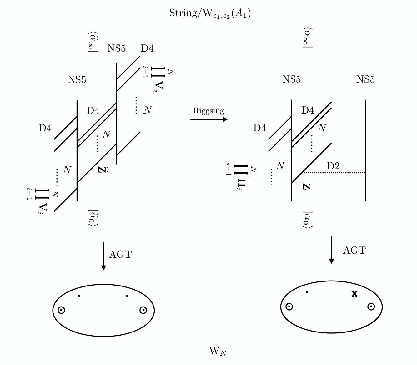
The brane picture is also useful for understanding in which sense the AGT relation happen to be orthogonal (literally) to our description: the stack of $N$ D4 support the higher rank algebra $\text{W}_{N}$ , with each NS5 intersecting the D4 describing a rank $N-1$ full puncture and a rank $1$ simple puncture. After Higgsing, the emerging D2 is associate to the simple puncture which has turned to fully-degenerate.

Generally, for 4d $\mathcal{N}=2$ $A$ -shaped quivers and unitary gauge groups, the duality we have just described can be generalized to an equivalence of $(M+2)$ -point functions in $\text{W}_{N}$ and $(N+2)$ -point functions in $\text{W}_{{\epsilon}_{1},{\epsilon}_{2}}(A_{M-1})$ . We also expect that a similar relation will hold for a wider class of surface defects as well Gomis:2016ljm. In the 5d/ $q$ -deformed setup, the origin of such interplay is known from the string perspective due to fiber/base/S-duality Katz:1997eq; Bao:2011rc, the algebraic viewpoint because of Miki’s automorphism of the DIM algebra, and the theory of integrable systems: the effect of the duality on the gauge theory side is simply to exchange the rank of the quiver with the rank of the gauge group, with a Lagrangian description existing in both frames; at the quantum group level, the duality simply exchanges two algebras in the same family and their correlation functions; in integrable systems of fully trigonometric type, spectral duality acts within the same class. Instead, in the 4d/ ${\epsilon}$ -deformed setup the duality changes the type of algebras involved, and the very existence of the duality is far less understood. This is because the existence of only one frame where a conventional gauge theory description seems to be valid. In fact, at codim-2, the duality has been shown Zenkevich:2017ylb to look very much as Hori-Vafa mirror symmetry between gauged linear sigma models and Landau-Ginzburg theories Hori:2000kt; Aganagic:2001uw; Gomis:2012wy. On the algebraic side, the relation between our approach and AGT is ultimately to be found in the representation theory of the affine Yangian which underlies both constructions.

4.2 rRS model and dual Jack functions

In this last subsection, we would like to explore possible relations between $\text{W}_{{\epsilon}_{1},{\epsilon}_{2}}(\Xi)$ algebras associated to 4d/2d quiver gauge theories and quantum integrable systems. For simplicity, we focus on $A$ -type quivers only. A natural starting point in this direction is the observation that the $\text{W}_{q,t^{-1}}(A_{N})$ algebras were introduced in connection with the theory of Macdonald polynomials: in the CFT-limit $q\to 1$ , these reduce to Jack polynomials which are in one-to-one correspondence with $\text{W}_{N}$ singular vectors, while the former turns out to be in one-to-one correspondence with $\text{W}_{q,t^{-1}}(A_{N})$ singular vectors Awata:1995np; Awata:1995zk. Moreover, another characterization of these orthogonal polynomials is through the integrable systems they are related to: Macdonald or Jack polynomials are eigenfunctions of the trigonometric Ruijsenaars-Schneider (tRS) or Calogero-Moser-Sutherland (tCMS) models respectively.²¹²¹ 21 More precisely, they describe excitations over the vacuum. The vacuum wavefunction is simply a trigonometric $q/\beta$ -deformed Vandermonde determinant which can be stripped off. The connection to $\text{W}_{q,t^{-1}}(A_{N})$ and $\text{W}_{N}$ algebras goes through the bosonization formulas of the quantum Hamiltonians: once the Heisenberg oscillators are represented on the Fock space of symmetric functions by choosing the power sums basis, the non-diagonal part of the Hamiltonians can be expressed in terms of the algebra generators which annihilate the singular vectors constructed from the screening currents. Here, we aim at applying part of this logic to the case of the $\text{W}_{{\epsilon}_{1},{\epsilon}_{2}}(A_{N})$ algebra.

We are going to show that: $i)$ certain $\text{W}_{{\epsilon}_{1},{\epsilon}_{2}}(A_{N})$ free boson correlators are eigenfunctions of the rational Ruijsenaars-Scheider (rRS) system; $ii$ ) spectral duality between $\text{W}_{{\epsilon}_{1},{\epsilon}_{2}}(A_{N})$ and $\text{W}_{N}$ correlators corresponds to the PQ-duality exchanging coordinates and momenta between the rRS and tCMS models.²²²² 22 Actually, the more appropriate model is the hyperbolic one. From our perspective, the difference amounts in the interpretation of the oscillators either as trigonometric/hyperbolic variables. The reality conditions become important when discussing the actual spectrum of the Hamiltonians, but they play a little role in the bosonization formulas as we always work in a complexified setup. The first relation follows from what we have just recalled, namely that certain screening integrals of the $\text{W}_{q,t^{-1}}(A_{N})$ algebra are tRS eigenfunctions. Upon taking the $\hbar$ -limit, one gets the singular vectors²³²³ 23 By analogy with the $q$ -deformed case, we continue to use the world singular vector even though we do not know the exact relation with the representation theory of the $\text{W}_{{\epsilon}_{1},{\epsilon}_{2}}(A_{N})$ algebra. of the $\text{W}_{{\epsilon}_{1},{\epsilon}_{2}}(A_{N})$ algebra (dual Jack functions) on the one side, and the corresponding rRS eigenfunctions on the other side. The second relation describes how the spectral/PQ-duality manifests itself on the level of integrable systems.²⁴²⁴ 24 In the context of 3d quiver gauge theories and tRS model, this and other aspects are extensively discussed in Gaiotto:2013bwa; Bullimore:2014awa; Koroteev:2019byp. The tRS model is known to be PQ-self-dual as the dependance on coordinates and momenta is trigonometric/trigonometric. On the one hand, after the $\hbar$ -limit the tRS Hamiltonian turns into the rRS Hamiltonian in which the dependance on coordinates becomes rational (the circle on which the coordinates live is decompactified). On the other hand, the tCMS model arises in the dual CFT-limit of tRS, in which it is the dependance on momenta becoming rational. Given the action of PQ-duality, it is natural that the two different limits of tRS are dual to each other: this is the remnant of the self-duality which is broken by the limiting procedures.

In order to develop these points, let us start by recalling the Macdonald/tRS Hamiltonian for a system of $N$ particles with positions $x_{i}$ , which we take to be

H_{\text{t}}\equiv\sum_{i=1}^{N}\prod_{j\neq i}\frac{tx_{i}-x_{j}}{x_{i}-x_{j}}\ q^{x_{i}\partial_{x_{i}}}~,

(112)

which in the $\hbar$ -limit reduces to the rRS Hamiltonian

H_{2}\equiv\sum_{i=1}^{N}\prod_{j\neq i}\frac{{\epsilon}_{2}+X_{i}-X_{j}}{X_{i}-X_{j}}\ {\rm e}^{-{\epsilon}_{1}\partial_{X_{i}}}.

(113)

It is an interesting problem to express this operator in terms of $\text{W}_{{\epsilon}_{1},{\epsilon}_{2}}(A_{N})$ generators, as our construction suggests, but we do not attempt to do that here. Instead, our goal is to algorithmically construct its eigenfunctions in terms of the $\text{W}_{{\epsilon}_{1},{\epsilon}_{2}}(A_{N})$ screening charges and compute the resulting eigenvalues. Let us begin with a trivial example, namely the 1-body Hamiltonian whose eigenfunction is

\psi(X_{1}|z_{1})\sim z_{1}^{-X_{1}/{\epsilon}_{1}}~,

(114)

with eigenvalue $E_{2}=z_{1}$ . This result holds up to multiplication by a periodic function of the coordinate with period ${\epsilon}_{1}$ . As a less trivial yet simple example, let us take the 2-body Hamiltonian, for which it can be verified that²⁵²⁵ 25 We recall that, if a function $f(x)$ has a pole at $x=x_{0}$ , then $f(x_{0})$ denotes its residue.

\psi(X_{1},X_{2}|z_{1},z_{2})\sim z_{2}^{-\frac{X_{1}+X_{2}}{\epsilon_{1}}}\left(\frac{z_{1}}{z_{2}}\right)^{-\frac{X_{1}}{{\epsilon}_{1}}}\ \frac{\Gamma_{1}(0|{\epsilon}_{1})\Gamma_{1}(X_{2}-X_{1}|{\epsilon}_{1})}{\Gamma_{1}(-{\epsilon}_{2}|{\epsilon}_{1})\Gamma_{1}(-{\epsilon}_{2}+X_{2}-X_{1}|{\epsilon}_{1})}\times\\ \times{}_{2}F_{1}\left[\begin{smallmatrix}\epsilon_{+},&\epsilon_{+}+X_{1}-X_{2}\\ {\epsilon}_{1},&{\epsilon}_{1}+X_{1}-X_{2}\end{smallmatrix}\left|\frac{z_{2}}{z_{1}}\right.\right]

(115)

is an eigenfunction with eigenvalue $E_{2}=z_{1}+z_{2}$ . This directly follows from the hypergeometric equation and contiguous recurrence relations. Due to the symmetry of the problem, we can of course get another solution by exchanging $X_{1}\leftrightarrow X_{2}$ , and we can give an integral representation of the solutions as follows

\psi(X_{1},X_{2}|z_{1},z_{2})\equiv z_{2}^{-\frac{X_{1}+X_{2}}{\epsilon_{1}}}\oint_{\mathcal{C}_{i}}\frac{{\rm d}s}{2\pi{\rm i}}\ \left(\frac{z_{1}}{z_{2}}\right)^{-\frac{s}{{\epsilon}_{1}}}\prod_{j=1}^{2}\frac{\Gamma_{1}(X_{j}-s|{\epsilon}_{1})}{\Gamma_{1}(-{\epsilon}_{2}+X_{j}-s|{\epsilon}_{1})}~,

(116)

where the enclosed poles are at $s=X_{i}+n{\epsilon}_{1}$ , $n\in\mathbb{Z}_{\geq 0}$ . These two expressions are nothing but a basis of the 4-point functions with two degenerate fields of the ${\epsilon}$ -Virasoro algebra, constructed using a single screening current. We have already shown that such free field conformal blocks are spectral dual to the conformal blocks of the ordinary Virasoro algebra, which are in turn eigenfunctions of the 2-body tCMS system as we recall below.

More generally, the $N$ -body eigenfunctions can be obtained by induction using the kernel function for the rRS Hamiltonian²⁶²⁶ 26 In the trigonometric case, similar kernel functions arise from completeness of Macdonald/Jack/Schur functions. It is an interesting question whether this applies to the present case as well, of which we do not know the answer.

\Pi(\vec{Y},\vec{X})\equiv\prod_{i=1}^{N}\prod_{j=1}^{M}\frac{\Gamma_{1}(X_{i}-Y_{j}|{\epsilon}_{1})}{\Gamma_{1}(-{\epsilon}_{2}+X_{i}-Y_{j}|{\epsilon}_{1})}~.

(117)

The derivation is very similar to that in the trigonometric case (we refer to Bullimore:2014awa; Koroteev:2015dja; Zenkevich:2017ylb for the discussion in the context of 3d gauge theories). Indeed, consider the action of the rRS Hamiltonian in $X$ variables on the kernel function (117). Using the recurrence relation for the $\Gamma_{1}$ function we get

H_{2}^{(X)}\Pi(\vec{Y},\vec{X})=\sum_{i=1}^{N}\prod_{j\neq i}^{N}\frac{X_{i}-X_{j}-{\epsilon}_{2}}{X_{i}-X_{j}}\prod_{k=1}^{M}\frac{X_{i}-Y_{k}}{X_{i}-Y_{k}-\epsilon_{2}}\ \Pi(\vec{Y},\vec{X})~.

(118)

We can notice that the rational function in (118) can be written as a contour integral

H_{2}^{(X)}\Pi(\vec{Y},\vec{X})=-\oint_{\mathcal{C}_{X}}\frac{{\rm d}z}{2\pi{\rm i}\epsilon_{2}}\prod_{j=1}^{N}\frac{z-X_{j}-{\epsilon}_{2}}{z-X_{j}}\prod_{k=1}^{M}\frac{z-Y_{k}}{z-Y_{k}-\epsilon_{2}}\ \Pi(\vec{Y},\vec{X})~,

(119)

where $\mathcal{C}_{X}$ encircles the poles at $X_{i}$ , $i=1,\dots,N$ . Expanding the contour we get residues at $z=Y_{i}$ and at $z=\infty$ , namely

		$\displaystyle\oint_{\mathcal{C}_{Y}}\frac{{\rm d}z}{2\pi{\rm i}\epsilon_{2}}\prod_{j=1}^{N}\frac{z-X_{j}-{\epsilon}_{2}}{z-X_{j}}\prod_{k=1}^{M}\frac{z-Y_{k}}{z-Y_{k}-\epsilon_{2}}=\sum_{k=1}^{M}\prod_{j\neq k}^{M}\frac{Y_{k}-Y_{j}+{\epsilon}_{2}}{Y_{k}-Y_{j}}\prod_{l=1}^{N}\frac{Y_{k}-X_{l}}{Y_{k}-X_{l}+\epsilon_{2}}~,$		(120)
		$\displaystyle-\oint_{\mathcal{C}_{\infty}}\frac{{\rm d}z}{2\pi{\rm i}\epsilon_{2}}\prod_{j=1}^{N}\frac{z-X_{j}-{\epsilon}_{2}}{z-X_{j}}\prod_{k=1}^{M}\frac{z-Y_{k}}{z-Y_{k}-\epsilon_{2}}=N-M~.$		(121)

Summing up two contributions (120) and (121) we get

H_{2}^{(X)}\Pi(\vec{Y},\vec{X})=\left[N-M+\sum_{k=1}^{M}\prod_{j\neq k}^{M}\frac{Y_{k}-Y_{j}+{\epsilon}_{2}}{Y_{k}-Y_{j}}\prod_{l=1}^{N}\frac{Y_{k}-X_{l}}{Y_{k}-X_{l}+\epsilon_{2}}\right]\Pi(\vec{Y},\vec{X})=\\ =\left[N-M+\sum_{k=1}^{M}\prod_{j\neq k}^{M}\frac{Y_{k}-Y_{j}+{\epsilon}_{2}}{Y_{k}-Y_{j}}e^{-\epsilon_{1}\partial_{Y_{k}}}\right]\Pi(\vec{Y},\vec{X})=\left[N-M+(H_{2}^{(Y)})^{{\dagger}}\right]\Pi(\vec{Y},\vec{X})~,

(122)

where the conjugate of the rRS Hamiltonian is defined using the following scalar product on wavefunctions²⁷²⁷ 27 Strictly speaking, we should carefully specify the class of allowed functions as we need some control over the analytic properties. However, here we only act on kernel functions which are well under control.

\langle f|g\rangle\equiv\oint\frac{{\rm d}^{N}X}{(2\pi{\rm i})^{N}}\Delta^{(\epsilon_{1},\epsilon_{2})}(\vec{X})f(\vec{X})g(\vec{X})~,

(123)

with measure determined by the ${\epsilon}$ -deformed version of the Vandermonde determinant

\Delta^{(\epsilon_{1},\epsilon_{2})}(\vec{X})\equiv\prod_{i\neq j}^{N}\frac{\Gamma_{1}(X_{i}-X_{j}-\epsilon_{2}|\epsilon_{1})}{\Gamma_{1}(X_{i}-X_{j}|\epsilon_{1})}~.

(124)

The integral representation of the multiparticle wavefunction is thus given by

\psi(\vec{X}^{(N)}|\vec{z}^{(N)})\equiv z_{N}^{-\frac{\sum_{i=1}^{N}X_{i}^{(N)}}{\epsilon_{1}}}\times\\ \times\oint\prod_{a=1}^{N-1}\frac{{\rm d}X^{(a)}}{(2\pi{\rm i})^{N/2}}\prod_{a=1}^{N-1}\left(\frac{z_{a}}{z_{a+1}}\right)^{-\frac{\sum_{i=1}^{a}X^{(a)}_{i}}{\epsilon_{1}}}\Delta^{(\epsilon_{1},\epsilon_{2})}(\vec{X}^{(a)})\Pi(\vec{X}^{(a)},\vec{X}^{(a+1)})~.

(125)

In fact, the $N$ -body rRS Hamiltonian $H_{2}^{(X^{(N)})}$ acts on the last kernel, and using the identity (122) it can be expressed through the conjugate Hamiltonian acting on $X^{(N-1)}$ variables. The $\epsilon$ -deformed Vandermonde determinant can then be used to convert the conjugate Hamiltonian back to the original one. Moving the Hamiltonian sequentially from right to left one eventually proves that (125) is indeed an eigenfunction with eigenvalue

E_{2}=z_{N}\left(1+\frac{z_{N-1}}{z_{N}}\left(1+\frac{z_{N-2}}{z_{N-1}}(\ldots)\right)\right)=\sum_{i=1}^{N}z_{i}~.

(126)

Remark. The eigenfunctions of the tRS model describe vortex partition functions of the 3d self-mirror $T[\text{U}(N)]$ theory Bullimore:2014awa, the S-duality wall of 4d $\mathcal{N}=4$ SYM. In this setup, the tRS Hamiltonians and eigenvalues represent the action of bulk ’t Hooft and Wilson loop operators at the interface. This theory also arises from maximal Higgsing of the 5d square theory $\text{U}(N)^{N-1}$ Zenkevich:2017ylb; Aprile:2018oau, and it can also be seen a full monodromy defect in 5d $\mathcal{N}=1^{*}$ SYM Bullimore:2014awa. Similarly, following the algebra/gauge dictionary of section 3, the eigenfunctions of the rRS model which we have constructed also match vortex partition functions of the 2d $\mathcal{N}=(2,2)$ theory arising from maximal Higgsing of the 4d square theory. This property has been known for a long time negut2009; Braverman:2010ei, and the embedding of the theory as a full monodromy defect in 4d $\mathcal{N}=2^{*}$ SYM was further studied in Nawata:2014nca. We also refer to Honda:2013uca the for gauge theory interpretation of the Hamiltonians.

We now turn to describing the spectral dual system. The dual tCMS Hamiltonian²⁸²⁸ 28 This is the second in the hierarchy of CMS integrals of motion. The first Hamiltonian $\tilde{H}_{1}=\sum_{i=1}^{N}\epsilon_{1}z_{i}\partial_{z_{i}}$ just counts the total homogeneous degree of the wavefunction in $z_{i}$ .

\tilde{H}_{2}\equiv\sum_{i=1}^{N}(\epsilon_{1}z_{i}\partial_{z_{i}})^{2}-\sum_{i\neq j}\frac{\epsilon_{2}\left(\epsilon_{2}+\epsilon_{1}\right)z_{i}z_{j}}{(z_{i}-z_{j})^{2}}

(127)

acts on the $z_{i}$ variables, but it is non-trivial to see directly from the given integral representation that (125) (up to a rescaling which we could not fix so far) is in fact its eigenfunction as well. In the 2-particle case, one can deduce the result from the hypergeometric differential equation

\tilde{H}_{n=1,2}\tilde{\psi}(X_{1},X_{2}|z_{1},z_{2})=(X_{1}^{n}+X_{2}^{n})\tilde{\psi}(X_{1},X_{2}|z_{1},z_{2})~,

(128)

which allows us to fix the correct rescaling factor as (essentially, the vacuum wavefunction which is usually stripped off from the very beginning)

\tilde{\psi}(X_{1},X_{2}|z_{1},z_{2})\equiv\frac{z_{2}}{z_{1}}\left(1-\frac{z_{2}}{z_{1}}\right)^{\frac{\epsilon_{+}}{\epsilon_{1}}}\psi(X_{1},X_{2}|z_{1},z_{2})~.

(129)

Another way of proving (128) is to first use the Euler transformation on the hypergeometric function in (116)

{}_{2}F_{1}\left[\begin{smallmatrix}\epsilon_{+},&\epsilon_{+}+X_{1}-X_{2}\\ {\epsilon}_{1},&{\epsilon}_{1}+X_{1}-X_{2}\end{smallmatrix}\left|\frac{z_{2}}{z_{1}}\right.\right]=\left(1-\frac{z_{2}}{z_{1}}\right)^{-2\frac{\epsilon_{2}}{\epsilon_{1}}-1}{}_{2}F_{1}\left[\begin{smallmatrix}-\epsilon_{2},&-\epsilon_{2}+X_{1}-X_{2}\\ {\epsilon}_{1},&{\epsilon}_{1}+X_{1}-X_{2}\end{smallmatrix}\left|\frac{z_{2}}{z_{1}}\right.\right]~,

(130)

and then use the Euler-Selberg integral representation

\tilde{\psi}(X_{1},X_{2}|z_{1},z_{2})\sim(z_{1}z_{2})^{-\frac{X_{1}}{\epsilon_{1}}}\frac{z_{2}}{z_{1}}(z_{1}-z_{2})^{-\frac{\epsilon_{2}}{\epsilon_{1}}}\frac{{\rm e}^{\frac{{\rm i}\pi}{{\epsilon}_{1}}(X_{2}-X_{1})}}{\sin\frac{\pi}{{\epsilon}_{1}}(X_{2}-X_{1})}\frac{\Gamma_{1}\left(X_{2}-X_{1}+\epsilon_{+}|\epsilon_{1}\right)}{\Gamma_{1}\left(X_{2}-X_{1}-\epsilon_{2}|\epsilon_{1}\right)}\times\\ \times\oint_{\gamma_{1}}{\rm d}x\,x^{\frac{X_{1}-X_{2}-\epsilon_{+}}{\epsilon_{1}}}(z_{2}-x)^{\frac{\epsilon_{2}}{\epsilon_{1}}}\left(z_{1}-x\right)^{\frac{\epsilon_{2}}{\epsilon_{1}}}~,

(131)

where $\gamma_{1}$ is the Pochhammer contour wrapping two times around $0$ and $z_{1}$ . In general, the appropriately rescaled rRS eigenfunction is also an eigenfunction of the tCMS, with eigenvalues

\tilde{E}_{n}=\sum_{i=1}^{N}X_{i}^{n}.

(132)

The dual integral representation can be written recursively using the kernel function

\text{P}(\vec{z},\vec{w})\equiv\prod_{i=1}^{N}\prod_{j=1}^{M}\frac{1}{(z_{i}-w_{j})^{-\frac{\epsilon_{2}}{\epsilon_{1}}}}~,

(133)

and the corresponding Euler-Selberg representation reads as

\tilde{\psi}(\vec{X}^{(N)}|\vec{z}^{(N)})\sim\left(\prod_{i=1}^{N}z_{i}\right)^{-\frac{X_{1}}{\epsilon_{1}}}\times\\ \times\oint\prod_{a=1}^{N-1}\frac{{\rm d}\ln z^{(a)}}{(2\pi{\rm i})^{N/2}}\prod_{a=1}^{N-1}\left(\prod_{i=1}^{a}z_{i}^{(a)}\right)^{\frac{X_{a}-X_{a+1}-\epsilon_{+}}{\epsilon_{1}}}\Delta(\vec{z}^{(a)})^{-2\frac{\epsilon_{2}}{\epsilon_{1}}}\ \text{P}(\vec{z}^{(a)},\vec{z}^{(a+1)})~,

(134)

where $\Delta(\vec{z})\equiv\prod_{i<j}(z_{i}-z_{j})$ is the standard Vandermonde determinant.

From the last expression, it is manifest that the polynomial eigenfunctions, a.k.a. Jack polynomials, can be obtained by putting the rRS positions $\vec{X}^{(N)}$ on a lattice. However, this can also be seen in the Mellin-Barnes representation which is adapted to the rRS models instead. For instance, in the 2-body case, the representation (116) immediately tells us that if $X_{1}-X_{2}+\epsilon_{+}=-n\epsilon_{1}$ with $n\in\mathbb{Z}_{\geq 0}$ , then the hypergeometric series truncates and becomes a polynomial in $z_{2}/z_{1}$ . The first few Jack polynomials explicitly read

$\displaystyle\psi(X_{1},X_{1}+\epsilon_{1}+\epsilon_{2})$	$\displaystyle\sim 1,$	(135)
$\displaystyle\psi(X_{1},X_{1}+2\epsilon_{1}+\epsilon_{2})$	$\displaystyle\sim z_{1}+z_{2}=p_{1},$	(136)
$\displaystyle\psi(X_{1},X_{1}+3\epsilon_{1}+\epsilon_{2})$	$\displaystyle\sim z_{1}^{2}+z_{2}^{2}+\frac{2(\epsilon_{1}+\epsilon_{2})}{(2\epsilon_{1}+\epsilon_{2})}z_{1}z_{2}=\frac{{\epsilon}_{1}}{2{\epsilon}_{1}+{\epsilon}_{2}}\left(p_{2}+\frac{\epsilon_{1}+\epsilon_{2}}{\epsilon_{1}}p_{1}^{2}\right)~,$	(137)
$\displaystyle\cdots$		(138)

where $p_{n}=z_{1}^{n}+z_{2}^{n}$ denotes the power sum basis.

Before concluding this section, let us point out that there is a further natural limit one can take in the rRS model, which from the gauge theory perspective corresponds to a semi-classical limit removing the disk equivariant parameter. This is the non-relativistic limit ${\epsilon}_{1}\to 0$ with $\beta\equiv-{\epsilon}_{2}/{\epsilon}_{1}$ fixed²⁹²⁹ 29 From a 2d CFT perspective, this is the heavy-charge-limit as $X/{\epsilon}_{1}\to\infty$ or the classical limit as $c\to\infty$ .

H_{2}\to\sum_{i}\partial_{X_{i}}^{2}+\sum_{i\neq j}\frac{\beta}{X_{i}-X_{j}}\partial_{X_{i}}~,

(139)

at quadratic order in ${\epsilon}_{1}$ . Upon taking the limit, the ${\epsilon}$ -deformed Vandermonde determinant coming from the 2-point function of the $\text{W}_{{\epsilon}_{1},{\epsilon}_{2}}$ screening currents reduces to its $\beta$ -deformed version

\Delta^{({\epsilon}_{1},{\epsilon}_{2})}(\vec{X})\to\prod_{i<j}(X_{i}-X_{j})^{2\beta}~,

(140)

and similarly for the generalized kernel (potential terms)

\prod_{i,f}\frac{\Gamma_{1}(X_{i}-Y_{f}|{\epsilon}_{1})}{\Gamma_{1}(X_{i}-Y_{f}-{\epsilon}_{2}\alpha_{f}|{\epsilon}_{1})}\to\prod_{i,f}(X_{i}-Y_{f})^{-\beta\alpha_{f}}~.

(141)

In particular, this means that in this limit the $\text{W}_{{\epsilon}_{1},{\epsilon}_{2}}$ free boson correlators collapse to ordinary 2d CFT Dotsenko-Fateev matrix models, and $\text{W}_{{\epsilon}_{1},{\epsilon}_{2}}$ algebras to ordinary W algebras. In the example discussed before, the (dual) positions of the matrix model correspond to the coordinates of the rRS model, while all the (dual) momenta are set to be degenerate (i.e. fixed by $\beta$ ). The non-relativistic rRS Hamiltonian is also equivalent to the rCMS model upon stripping off the vacuum wavefunction. This can be directly seen by performing this similarity transformation on the tCMS Hamiltonian

\tilde{H}_{2}\simeq\sum_{i=1}^{N}({\epsilon}_{1}z_{i}\partial_{z_{i}})^{2}-{\epsilon}_{1}{\epsilon}_{2}\sum_{i\neq j}\frac{z_{i}+z_{j}}{z_{i}-z_{j}}z_{i}\partial_{z_{i}}~,

(142)

and then taking the rational limit by setting $z_{i}\equiv\exp({\epsilon}_{1}y_{i})$ and keeping the constant terms in ${\epsilon}_{1}$

\tilde{H}_{2}\to\sum_{i}\partial_{y_{i}}^{2}+\sum_{i\neq j}\frac{\beta}{y_{i}-y_{j}}\partial_{y_{i}}~.

(143)

We see that, having now a rational/rational model, this is again self-dual. However, the non-relativistic limit has different meanings: in the rRS side, it rescales the positions by a very large parameter (i.e. heavy-charge regime), while in the tCMS side it pushes the coordinates close to the unit circle (i.e. decompactification regime).

5 Conclusions and future directions

In this paper, we have introduced a class of algebras which are naturally associated to any 4d $\mathcal{N}=2$ quiver gauge theory with unitary groups. Our construction is inspired by the parallel KP construction regarding the 5d dimensional case and quiver $\text{W}_{q,t^{-1}}$ algebras. In fact, it essentially follows from their construction upon a suitable implementation of the dimensional reduction on the algebraic side, which we have called $\hbar$ -limit. This is not the CFT-limit which reproduces the well-known AGT relation, rather our approach can be thought as its spectral dual (in the sense of integrable systems) and the resulting $\text{W}_{{\epsilon}_{1},{\epsilon}_{2}}$ algebra are dual to ordinary W algebra, hence sharing the same conformal blocks. Our construction has the advantage of being directly related to instanton calculus, while such connection is not manifest in the AGT framework. This is non-trivial interplay is partially due to the lack of manifest and simple $\mathbb{SL}(2,\mathbb{Z})$ covariance at various levels when reducing from five to four dimensions. At the level of associated integrable systems, this is due to the lack of spectral-self-duality, which is restored only after taking a semi-classical limit.

There are a number of open questions and further directions to explore. Probably, the most urgent one would be a clearer understanding of $\text{W}_{{\epsilon}_{1},{\epsilon}_{2}}$ algebras from the 2d CFT perspective. Intuitively, we may expect that they govern the integrability or recurrence relations of correlators by playing an analogous role in weight space as W algebras do on the world-sheet. The precise mapping between the continuous free boson formalism and the discrete one might be crucial for this purpose and for establishing direct connections with previous and recent works concerning the affine Yangian and $\text{W}/\text{W}_{1+\infty}$ algebras Gaiotto:2017euk; Prochazka:2017qum. Also, this would probably provide us with a more solid mathematical characterization of our algebras. Moreover, $\text{W}_{{\epsilon}_{1},{\epsilon}_{2}}$ algebras might be a helpful machinery in trying to solve Toda theories through gauge or topological string theory techniques Kozcaz:2010af; Mitev:2014isa; Isachenkov:2014eya; Coman:2019eex.

Another very interesting direction to consider is what our construction has to say about the WZW/Liouville correspondence Ribault:2005wp; Hikida:2007tq. According to AGT Alday:2010vg; Kozcaz:2010yp, this relation appears when considering different types of codim-2 defects which can be engineered by either coupling d.o.f. to the bulk or as monodromy defects Gukov:2006jk; Braverman:2004vv; Braverman:2004cr. The equivalence of the conformal blocks (through a generalized Fourier transform) is then a manifestation of an IR duality between the two gauge theory descriptions Frenkel:2015rda. In a particular example involving the 5d $\mathcal{N}=1^{*}$ theory coupled to codim-2 defects, this has been related to Witten S-duality action Witten:2003ya. Notably, this type of duality has also been related to various aspects of the (quantum) geometric Langlands correspondence Kapustin:2006pk. In order to understand why we expect our work to be related to these topics, it is useful to recall that recently a (quantum) $q$ -geometric Langlands correspondence has been put forward Aganagic:2017smx; Elliott:2018yqm. A convenient way to think about it is as a correspondence between $q$ -affine (off the critical level) and $\text{W}_{q,t^{-1}}$ conformal blocks for Langlands dual groups, which is strongly reminiscent of the WZW/Liouville setup. A key role from this perspective is played by the elliptic stable envelopes Aganagic:2016jmx, which provide (part of) the connection between the two sides. Since these objects naturally arise when studying certain aspects of 3d mirror symmetry Rimanyi:2019zyi, in turn closely related to spectral duality, we naturally expect that $\text{W}/\text{W}_{{\epsilon}_{1},{\epsilon}_{2}}$ duality will fit into another intermediate layer between geometric Langlands and its $q$ -deformation. In order to fully explore this possibility, the inclusion of diverse surface defects and non-simply laced algebras in our setup would be desirable Kimura:2017hez; Haouzi:2017vec.

Finally, another direction worth to be explored is whether T-duality of the little string can offer another (dual) derivation of the AGT relations, along the lines of Cordova:2016cmu but now starting from the low energy description provided by 6d SYM. This may be achieved by exploiting the ideas developed in Costello:2018txb.

Acknowledgements.

The authors thanks S. Pasquetti, E. Pomoni, V. Schomerus and J. Teschner for valuable discussions. FN thanks CIRM for the hospitality during the BPS/CFT workshop where part of this work was done. YZ acknowledges the hospitality of DESY theory department where part of this work was done. FN is supported by DESY theory group. YZ is partially supported by RFBR grants 19-02-00815, 18-51-05015-Arm, 19-51-50008-YaF, and 19-51-18006-Bolg.

Appendix A Special functions

In this appendix, we present a summary of the special functions used in the main text and some of their properties. For a full account we refer to Narukawa:2003.

Gamma function: integral definition and properties.

\Gamma_{1}(X|\omega)\equiv\frac{{\rm e}^{B_{11}(X|\omega)\ln\omega}}{\sqrt{2\pi}}\ \Gamma(X/\omega)~,

(144)

B_{11}(X|\omega)\equiv\frac{X}{\omega}-\frac{1}{2}=-\oint_{0}\frac{{\rm d}k}{2\pi{\rm i}}\frac{{\rm e}^{-kX}}{k(1-{\rm e}^{-\omega k})}~.

(145)

For ${\rm Re}(X)>0$ , ${\rm Re}(\omega)>0$ we have the integral representation

	$\displaystyle\ln\Gamma_{1}(X\|\omega)=$	$\displaystyle\ -\gamma B_{11}(X\|\omega)+\oint_{\mathcal{C}}\frac{{\rm d}k}{2\pi{\rm i}}\ln(-k)\frac{{\rm e}^{-kX}}{k(1-{\rm e}^{-\omega k})}={}$
	$\displaystyle=$	$\displaystyle\ -\gamma B_{11}(X\|\omega)+\oint_{\mathcal{C}}\frac{{\rm d}k}{2\pi{\rm i}k}\ln(-k)\frac{{\rm e}^{-k(X-\omega/2)}}{2\sinh(\omega k/2)}~,$		(146)

Therefore

\ln\Gamma(X/\omega)=\oint_{\mathcal{C}}\frac{{\rm d}k}{2\pi{\rm i}}\ln(-k)\frac{{\rm e}^{-kX}}{k(1-{\rm e}^{-\omega k})}-(\gamma+\ln\omega)B_{11}(X|\omega)+\ln\frac{1}{\sqrt{2\pi}}~.

(147)

It is useful to note that

\Gamma_{1}(X|\omega)\Gamma_{1}(\omega-X|\omega)=\frac{1}{S_{1}(X|\omega)}\equiv\frac{1}{2\sin(\pi X/\omega)}~.

(148)

Gamma function: series definition.

Let us consider the multiple $\zeta$ -function, which is the meromorphic analytic continuation to the complex $s$ -plane of the series

\zeta(s;X|\vec{\omega})\equiv\sum_{\vec{k}\in\mathbb{Z}^{r}_{\geq 0}}(\vec{k}\cdot\vec{\omega}+X)^{-s}~.

(149)

The Hurwitz $\zeta$ -function is $\zeta(s;X|1)$ , the Riemann $\zeta$ -function is $\zeta(s;1|1)$ . The series is convergent for $\text{Re}(s)>r$ and generic complex $\vec{\omega}$ all on the same side of a line through the origin. Since it is holomorphic at $s=0$ , one can define the multiple Gamma function through

\Gamma_{r}(X|\vec{\omega})\equiv\exp\left(\zeta^{\prime}(s;X|\vec{\omega})|_{s=0}\right)~,

(150)

where the derivative is w.r.t. the first argument. From this definition, we also get a formal series representation of the Log Gamma function, namely

\ln\Gamma_{1}(a+X|\omega)=\zeta^{\prime}(0;a|\omega)-X\sum_{k\geq 0}(k\omega+a)^{-1}+\sum_{j\geq 2}\frac{(-1)^{j}}{j}\zeta(j;a|\omega)X^{j}~.

(151)

The linear term in $X$ is divergent and needs to be interpreted as

\lim_{s\to 0}\frac{\zeta(1+s;a|\omega)+\zeta(1-s;a|\omega)}{2}=-\omega^{-1}\psi_{0}(a/\omega)~,

(152)

where $\psi_{0}(X)=\Gamma^{\prime}(X)/\Gamma(X)$ is the digamma function. Therefore we get the series expansion

\ln\Gamma_{1}(a+X|\omega)=\sum_{j\geq 0}\hat{\zeta}(j;a|\omega)\frac{X^{j}}{j!}~,

(153)

where we defined

\hat{\zeta}(j;a|\omega)\equiv\left\{\begin{array}[]{ll}(-1)^{j}\zeta(j;a|\omega)\Gamma(j)&j>1\\ \omega^{-1}\psi_{0}(a/\omega)&j=1\\ \zeta^{\prime}(0;a|\omega)&j=0\end{array}\right.~,

(154)

A useful identity is

\zeta(s;a|\omega)\Gamma(s)=\int_{0}^{\infty}\frac{{\rm d}k}{k}\,\frac{k^{s}\,{\rm e}^{-k(a-\omega/2)}}{2\sinh(\omega k/2)}~,

(155)

which is convergent for $\text{Re}(s)>1$ , $\text{Re}(a-\omega/2)>0$ . For $s\to 1$ we may use (152) to define the l.h.s., for $s\to 0$ we may regularize the l.h.s. by defining it as $\zeta^{\prime}(0;a|\omega)$ .

$\Gamma_{q}$ function.

The $q$ -Pochhammer symbol can be defined by the infinite product

(x;q)_{\infty}\equiv\prod_{k=0}^{\infty}(1-q^{k}x)~,

(156)

for $|q|<1$ and by analytic continuation otherwise. The $\Gamma_{q}$ function is defined as

\Gamma_{q}(X)\equiv(1-q)^{1-X}\frac{(q;q)_{\infty}}{(q^{X};q)_{\infty}}~,

(157)

and it has the undeformed limit

\lim_{q\to 1}\Gamma_{q}(X)=\Gamma(X)~.

(158)

Appendix B Continuous vs. discrete basis

Suppose we want to reproduce the 2-point function (3.5) for ${\epsilon}$ -Virasoro

\displaystyle\mathbf{S}(X)\mathbf{S}(Y)=

\displaystyle\ :\mathbf{S}(X)\mathbf{S}(Y):\,\frac{\Gamma_{1}(X-Y-{\epsilon}_{2}|{\epsilon}_{1})\Gamma_{1}(X-Y+{\epsilon}_{1}|{\epsilon}_{1})}{\Gamma_{1}(X-Y|{\epsilon}_{1})\Gamma_{1}(X-Y+{\epsilon}_{+}|{\epsilon}_{1})}\,{\rm e}^{2\gamma\beta}~,

(159)

by using a more conventional discrete boson(s) instead of the continuous one as we considered in the main text. By looking at (153), we may employ a field $\mathbf{a}(X)$ defined by

	$\displaystyle\mathbf{a}(X)\equiv$	$\displaystyle\ \sum_{j\geq 0}(\mathbf{a}^{+}_{j}+(-1)^{j}\mathbf{a}^{-}_{j})\frac{X^{j}}{j!}~,{}$
	$\displaystyle[\mathbf{a}^{+}_{j},\mathbf{a}^{-}_{\ell}]\equiv$	$\displaystyle\ \frac{1}{k!\ell!}\Big(\hat{\zeta}(j+\ell;-{\epsilon}_{2}+{\rm i}0)-\hat{\zeta}(j+\ell;{\epsilon}_{+}+{\rm i}0)+\hat{\zeta}(j+\ell;{\epsilon}_{1}+{\rm i}0)-\hat{\zeta}(j+\ell;{\rm i}0)\Big)~,$		(160)

with the normal ordering prescription of pushing $\mathbf{a}^{\mp}_{j}$ to the left/right. The ${\rm i}0$ notation denotes a regularization which we remove after computing the normal ordering functions.

In the main text, we have been using a continuous boson to get the very same 2-point function

\mathbf{s}(X)=\mathchoice{{\vbox{\hbox{$\textstyle-$}}\kern-4.86108pt}}{{\vbox{\hbox{$\scriptstyle-$}}\kern-3.43057pt}}{{\vbox{\hbox{$\scriptscriptstyle-$}}\kern-2.908pt}}{{\vbox{\hbox{$\scriptscriptstyle-$}}\kern-2.76045pt}}\!\int{\rm d}k\,\frac{\mathbf{s}(k)\,{\rm e}^{-kX}}{2\sinh({\epsilon}_{1}k/2)}~,

(161)

together with a prescription to deal with the normal ordering of the modes around $k=0$ . Let us explore how the two approaches may be related. We may be tempted to identify

\mathbf{a}_{j+}\simeq(-1)^{j}\int_{>0}{\rm d}k\,k^{j}\,\frac{{\mathbf{s}}(k)}{2\sinh({\epsilon}_{1}k/2)}~,\quad\mathbf{a}_{j-}\simeq-\int_{>0}{\rm d}k\,k^{j}\,\frac{{\mathbf{s}}(-k)}{2\sinh({\epsilon}_{1}k/2)}~,

(162)

at least for $j>0$ . This is consistent with the resulting commutator

[\mathbf{a}_{j+},\mathbf{a}_{\ell-}]\simeq(-1)^{j}\int_{0}^{\infty}\frac{{\rm d}k}{k}\,k^{j+\ell}\,\frac{\sinh({\epsilon}_{2}k/2)\ 2\cosh({\epsilon}_{+}k/2)}{\sinh({\epsilon}_{1}k/2)}~

(163)

thanks to (155). For $j+\ell=0,1$ , the identification is more problematic due to divergencies which needs to be interpreted. These divergences are expected from the small $k$ expansion of the continuous boson, where the dangerous terms indeed arise at linear order in spectral parameter. Let us also observe that we have not considered the zero modes properly here, which can indeed mix with the $j+\ell=0,1$ terms. Hopefully, a proper treatment of the zero modes will establish an exact correspondence between the formalism employing the continuous boson and a more traditional approach employing discrete modes.

Appendix C The generating and screening currents

In this appendix, we explicitly show that the ${\epsilon}$ -Virasoro generating a screening currents (66), (78) fulfill the relation (79). We first compute

\mathbf{Y}(Z+{\rm i}0)\mathbf{S}(X)=\ :\mathbf{Y}(Z)\mathbf{S}(X):\ \frac{X-Z-{\epsilon}_{2}/2}{X-Z+{\epsilon}_{2}/2-{\rm i}0}~,

(164)

and similarly

\mathbf{S}(X+{\rm i}0)\mathbf{Y}(Z)=\ :\mathbf{Y}(Z)\mathbf{S}(X):\ \frac{X-Z-{\epsilon}_{2}/2}{X-Z+{\epsilon}_{2}/2+{\rm i}0}~.

(165)

We recall that

\frac{1}{X\pm{\rm i}0}=\textrm{p.v.}\frac{1}{X}\mp{\rm i}\pi\delta(X)\ ,

(166)

so that we can write

\Big[\mathbf{Y}(Z),\mathbf{S}(X)\Big]=-2\pi{\rm i}{\epsilon}_{2}\ \delta(X-Z+{\epsilon}_{2}/2)\ :\mathbf{Y}(Z)\mathbf{S}(X):~,

(167)

and similarly

\Big[\mathbf{Y}(Z)^{-1},\mathbf{S}(X)\Big]=2\pi{\rm i}{\epsilon}_{2}\ \delta(X-Z-{\epsilon}_{2}/2)\ :\mathbf{Y}(Z)^{-1}\mathbf{S}(X):~.

(168)

Since we can identify ${\mathbf{s}}(k)=C(k)\mathbf{y}(k)$ , we finally get

\Big[\mathbf{T}(Z),\mathbf{S}(X)\Big]=\frac{{\rm d}_{{\epsilon}_{1}}}{{\rm d}_{{\epsilon}_{1}}X}\Big(\delta(X-Z)\mathbf{O}(X)\Big)~,

(169)

where

\mathbf{O}(X)=2\pi{\rm i}{\epsilon}_{1}{\epsilon}_{2}:\mathbf{Y}(X+{\epsilon}_{+}/2)\mathbf{S}(X+{\epsilon}_{1}/2):\ =\ {\epsilon}_{1}{\epsilon}_{2}:\mathbf{Y}(X-{\epsilon}_{+}/2)^{-1}\mathbf{S}(X-{\epsilon}_{1}/2):~.

(170)

References

(1) A. Lossev, N. Nekrasov, and S. L. Shatashvili, “Testing Seiberg-Witten solution,” arXiv:hep-th/9801061 [hep-th].
(2) G. W. Moore, N. Nekrasov, and S. Shatashvili, “D particle bound states and generalized instantons,” Commun. Math. Phys. 209 (2000) 77–95, arXiv:hep-th/9803265 [hep-th].
(3) G. W. Moore, N. Nekrasov, and S. Shatashvili, “Integrating over Higgs branches,” Commun. Math. Phys. 209 (2000) 97–121, arXiv:hep-th/9712241 [hep-th].
(4) A. Losev, N. Nekrasov, and S. L. Shatashvili, “Issues in topological gauge theory,” Nucl. Phys. B534 (1998) 549–611, arXiv:hep-th/9711108 [hep-th].
(5) N. A. Nekrasov, “Seiberg-Witten prepotential from instanton counting,” Adv. Theor. Math. Phys. 7 (2003) no. 5, 831–864, arXiv:hep-th/0206161 [hep-th].
(6) N. Nekrasov and A. Okounkov, “Seiberg-Witten theory and random partitions,” Prog. Math. 244 (2006) 525–596, arXiv:hep-th/0306238 [hep-th].
(7) A. Tsymbaliuk, “The affine yangian of $\mathfrak{gl}_{1}$ revisited,” arXiv:1404.5240 [math.RT].
(8) D. Maulik and A. Okounkov, “Quantum groups and quantum cohomology,” arXiv:1211.1287 [math.AG].
(9) O. Schiffmann and E. Vasserot, “Cherednik algebras, w algebras and the equivariant cohomology of the moduli space of instantons on $a^{2}$ ,” arXiv:1202.2756 [math.QA].
(10) T. Procházka, “ $\mathcal{W}$ -symmetry, topological vertex and affine Yangian,” JHEP 10 (2016) 077, arXiv:1512.07178 [hep-th].
(11) M. R. Gaberdiel, R. Gopakumar, W. Li, and C. Peng, “Higher Spins and Yangian Symmetries,” JHEP 04 (2017) 152, arXiv:1702.05100 [hep-th].
(12) H. Awata, M. Fukuma, Y. Matsuo, and S. Odake, “Representation theory of the W(1+infinity) algebra,” Prog. Theor. Phys. Suppl. 118 (1995) 343–374, arXiv:hep-th/9408158 [hep-th].
(13) M. R. Gaberdiel and R. Gopakumar, “An $AdS_{3}$ Dual for Minimal Model CFTs,” Phys. Rev. D83 (2011) 066007, arXiv:1011.2986 [hep-th].
(14) A. B. Zamolodchikov, “Infinite Additional Symmetries in Two-Dimensional Conformal Quantum Field Theory,” Theor. Math. Phys. 65 (1985) 1205–1213. [Teor. Mat. Fiz.65,347(1985)].
(15) L. F. Alday, D. Gaiotto, and Y. Tachikawa, “Liouville Correlation Functions from Four-dimensional Gauge Theories,” Lett. Math. Phys. 91 (2010) 167–197, arXiv:0906.3219 [hep-th].
(16) N. Wyllard, “A(N-1) conformal Toda field theory correlation functions from conformal N = 2 SU(N) quiver gauge theories,” JHEP 11 (2009) 002, arXiv:0907.2189 [hep-th].
(17) A. Mironov and A. Morozov, “On AGT relation in the case of U(3),” Nucl. Phys. B825 (2010) 1–37, arXiv:0908.2569 [hep-th].
(18) D. Gaiotto, “N=2 dualities,” JHEP 08 (2012) 034, arXiv:0904.2715 [hep-th].
(19) E. Carlsson and A. Okounkov, “Exts and Vertex Operators,”arXiv e-prints (Jan, 2008) arXiv:0801.2565, arXiv:0801.2565 [math.AG].
(20) N. A. Nekrasov and S. L. Shatashvili, “Supersymmetric vacua and Bethe ansatz,” Nucl. Phys. Proc. Suppl. 192-193 (2009) 91–112, arXiv:0901.4744 [hep-th].
(21) N. A. Nekrasov and S. L. Shatashvili, “Quantum integrability and supersymmetric vacua,” Prog. Theor. Phys. Suppl. 177 (2009) 105–119, arXiv:0901.4748 [hep-th].
(22) N. A. Nekrasov and S. L. Shatashvili, “Quantization of Integrable Systems and Four Dimensional Gauge Theories,” arXiv:0908.4052 [hep-th].
(23) N. Nekrasov, A. Rosly, and S. Shatashvili, “Darboux coordinates, Yang-Yang functional, and gauge theory,” Nucl. Phys. Proc. Suppl. 216 (2011) 69–93, arXiv:1103.3919 [hep-th].
(24) E. Carlsson, N. Nekrasov, and A. Okounkov, “Five dimensional gauge theories and vertex operators,” Moscow Math. J. 14 (2014) no. 1, 39–61, arXiv:1308.2465 [math.RT].
(25) N. Nekrasov, “BPS/CFT correspondence: non-perturbative Dyson-Schwinger equations and qq-characters,” JHEP 03 (2016) 181, arXiv:1512.05388 [hep-th].
(26) N. Nekrasov, “BPS/CFT correspondence II: Instantons at crossroads, moduli and compactness theorem,” Adv. Theor. Math. Phys. 21 (2017) 503–583, arXiv:1608.07272 [hep-th].
(27) N. Nekrasov, “BPS/CFT Correspondence III: Gauge Origami partition function and qq-characters,” Commun. Math. Phys. 358 (2018) no. 3, 863–894, arXiv:1701.00189 [hep-th].
(28) N. Nekrasov, “BPS/CFT correspondence IV: sigma models and defects in gauge theory,” Lett. Math. Phys. 109 (2019) no. 3, 579–622, arXiv:1711.11011 [hep-th].
(29) N. Nekrasov, “BPS/CFT correspondence V: BPZ and KZ equations from qq-characters,” arXiv:1711.11582 [hep-th].
(30) N. Nekrasov and V. Pestun, “Seiberg-Witten geometry of four dimensional N=2 quiver gauge theories,” arXiv:1211.2240 [hep-th].
(31) N. Nekrasov, V. Pestun, and S. Shatashvili, “Quantum geometry and quiver gauge theories,” Commun. Math. Phys. 357 (2018) no. 2, 519–567, arXiv:1312.6689 [hep-th].
(32) N. Seiberg and E. Witten, “Electric - magnetic duality, monopole condensation, and confinement in N=2 supersymmetric Yang-Mills theory,” Nucl. Phys. B426 (1994) 19–52, arXiv:hep-th/9407087 [hep-th]. [Erratum: Nucl. Phys.B430,485(1994)].
(33) N. Seiberg and E. Witten, “Monopoles, duality and chiral symmetry breaking in N=2 supersymmetric QCD,” Nucl. Phys. B431 (1994) 484–550, arXiv:hep-th/9408099 [hep-th].
(34) T. Kimura, “Double quantization of Seiberg-Witten geometry and W-algebras,” 2016. arXiv:1612.07590 [hep-th].
(35) H. Awata and Y. Yamada, “Five-dimensional AGT Conjecture and the Deformed Virasoro Algebra,” JHEP 01 (2010) 125, arXiv:0910.4431 [hep-th].
(36) A. Mironov, A. Morozov, S. Shakirov, and A. Smirnov, “Proving AGT conjecture as HS duality: extension to five dimensions,” Nucl. Phys. B855 (2012) 128–151, arXiv:1105.0948 [hep-th].
(37) F. Nieri, S. Pasquetti, and F. Passerini, “3d and 5d Gauge Theory Partition Functions as $q$ -deformed CFT Correlators,” Lett. Math. Phys. 105 (2015) no. 1, 109–148, arXiv:1303.2626 [hep-th].
(38) F. Nieri, S. Pasquetti, F. Passerini, and A. Torrielli, “5D partition functions, q-Virasoro systems and integrable spin-chains,” JHEP 12 (2014) 040, arXiv:1312.1294 [hep-th].
(39) M. Aganagic, N. Haouzi, C. Kozcaz, and S. Shakirov, “Gauge/Liouville Triality,” arXiv:1309.1687 [hep-th].
(40) M. Aganagic, N. Haouzi, and S. Shakirov, “ $A_{n}$ -Triality,” arXiv:1403.3657 [hep-th].
(41) M. Aganagic and S. Shakirov, “Gauge/Vortex duality and AGT,” in New Dualities of Supersymmetric Gauge Theories, J. Teschner, ed., pp. 419–448. 2016. arXiv:1412.7132 [hep-th].
(42) F. Benini, S. Benvenuti, and Y. Tachikawa, “Webs of five-branes and N=2 superconformal field theories,” JHEP 09 (2009) 052, arXiv:0906.0359 [hep-th].
(43) J. Shiraishi, H. Kubo, H. Awata, and S. Odake, “A Quantum deformation of the Virasoro algebra and the Macdonald symmetric functions,” Lett. Math. Phys. 38 (1996) 33–51, arXiv:q-alg/9507034 [q-alg].
(44) H. Awata, H. Kubo, S. Odake, and J. Shiraishi, “Quantum W(N) algebras and Macdonald polynomials,” Commun. Math. Phys. 179 (1996) 401–416, arXiv:q-alg/9508011 [q-alg].
(45) E. Frenkel and N. Reshetikhin, “Deformations of W-algebras associated to simple Lie algebras,” in eprint arXiv:q-alg/9708006. Aug., 1997.
(46) J. Ding and K. Iohara, “Generalization of drinfeld quantum affine algebras,”Letters in Mathematical Physics 41 (Jul, 1997) 181–193. https://doi.org/10.1023/A:1007341410987.
(47) K. Miki, “A $(q,\gamma)$ analog of the $w_{1+\infty}$ algebra,” Journal of Mathematical Physics 48 (2007) no. 12, 123520, https://doi.org/10.1063/1.2823979. https://doi.org/10.1063/1.2823979.
(48) J.-E. Bourgine, “Fiber-base duality from the algebraic perspective,” JHEP 03 (2019) 003, arXiv:1810.00301 [hep-th].
(49) B. Bastian, S. Hohenegger, A. Iqbal, and S.-J. Rey, “Triality in Little String Theories,” Phys. Rev. D97 (2018) no. 4, 046004, arXiv:1711.07921 [hep-th].
(50) S. H. Katz, A. Klemm, and C. Vafa, “Geometric engineering of quantum field theories,” Nucl. Phys. B497 (1997) 173–195, arXiv:hep-th/9609239 [hep-th].
(51) T. J. Hollowood, A. Iqbal, and C. Vafa, “Matrix models, geometric engineering and elliptic genera,” JHEP 03 (2008) 069, arXiv:hep-th/0310272 [hep-th].
(52) S. Katz, P. Mayr, and C. Vafa, “Mirror symmetry and exact solution of 4D N=2 gauge theories: 1.,” Adv. Theor. Math. Phys. 1 (1998) 53–114, arXiv:hep-th/9706110 [hep-th].
(53) L. Bao, E. Pomoni, M. Taki, and F. Yagi, “M5-Branes, Toric Diagrams and Gauge Theory Duality,” JHEP 04 (2012) 105, arXiv:1112.5228 [hep-th].
(54) M. Adams, J. Harnad, and J. Hurtubise, “Dual moment maps into loop algebras,” Letters in Mathematical Physics 20 (1990) no. 4, 299–308.
(55) J. P. Harnad, “Dual isomonodromic deformations and moment maps to loop algebras,” Commun. Math. Phys. 166 (1994) 337–366, arXiv:hep-th/9301076 [hep-th].
(56) M. Bertola, B. Eynard, and J. P. Harnad, “Duality, biorthogonal polynomials and multimatrix models,” Commun. Math. Phys. 229 (2002) 73–120, arXiv:nlin/0108049 [nlin-si].
(57) G. Wilson, “Bispectral commutative ordinary differential operators,” J. reine angew. Math 442 (1993) 177–204.
(58) M. Aganagic and N. Haouzi, “ADE Little String Theory on a Riemann Surface (and Triality),” arXiv:1506.04183 [hep-th].
(59) N. Haouzi and C. Schmid, “Little String Origin of Surface Defects,” JHEP 05 (2017) 082, arXiv:1608.07279 [hep-th].
(60) N. Haouzi and C. Kozçaz, “The ABCDEFG of Little Strings,” arXiv:1711.11065 [hep-th].
(61) Y. Zenkevich, “Generalized Macdonald polynomials, spectral duality for conformal blocks and AGT correspondence in five dimensions,” JHEP 05 (2015) 131, arXiv:1412.8592 [hep-th].
(62) A. Morozov and Y. Zenkevich, “Decomposing Nekrasov Decomposition,” JHEP 02 (2016) 098, arXiv:1510.01896 [hep-th].
(63) T. Kimura and V. Pestun, “Quiver W-algebras,” arXiv:1512.08533 [hep-th].
(64) T. Kimura and V. Pestun, “Fractional quiver W-algebras,” Lett. Math. Phys. 108 (2018) no. 11, 2425–2451, arXiv:1705.04410 [hep-th].
(65) T. Kimura, “Integrating over quiver variety and BPS/CFT correspondence,” arXiv:1910.03247 [hep-th].
(66) V. A. Alba, V. A. Fateev, A. V. Litvinov, and G. M. Tarnopolskiy, “On combinatorial expansion of the conformal blocks arising from AGT conjecture,” Lett. Math. Phys. 98 (2011) 33–64, arXiv:1012.1312 [hep-th].
(67) S. Mironov, A. Morozov, and Y. Zenkevich, “Generalized Jack polynomials and the AGT relations for the $SU(3)$ group,” JETP Lett. 99 (2014) 109–113, arXiv:1312.5732 [hep-th].
(68) P. Koroteev, “On Quiver W-algebras and Defects from Gauge Origami,” Phys. Lett. B800 (2020) 135101, arXiv:1908.04394 [hep-th].
(69) J. E. Bourgine and K. Zhang, “A note on the algebraic engineering of 4D $\mathcal{N}=2$ super Yang-Mills theories,” Phys. Lett. B789 (2019) 610–619, arXiv:1809.08861 [hep-th].
(70) R. Donagi and E. Witten, “Supersymmetric Yang-Mills theory and integrable systems,” Nucl. Phys. B460 (1996) 299–334, arXiv:hep-th/9510101 [hep-th].
(71) A. Gorsky, I. Krichever, A. Marshakov, A. Mironov, and A. Morozov, “Integrability and Seiberg-Witten exact solution,” Phys. Lett. B355 (1995) 466–474, arXiv:hep-th/9505035 [hep-th].
(72) A. Gorsky and A. Mironov, “Integrable many body systems and gauge theories,” arXiv:hep-th/0011197 [hep-th].
(73) A. Mironov, A. Morozov, Y. Zenkevich, and A. Zotov, “Spectral Duality in Integrable Systems from AGT Conjecture,” JETP Lett. 97 (2013) 45–51, arXiv:1204.0913 [hep-th]. [Pisma Zh. Eksp. Teor. Fiz.97,49(2013)].
(74) A. Mironov, A. Morozov, B. Runov, Y. Zenkevich, and A. Zotov, “Spectral Duality Between Heisenberg Chain and Gaudin Model,” Lett. Math. Phys. 103 (2013) no. 3, 299–329, arXiv:1206.6349 [hep-th].
(75) A. Mironov, A. Morozov, B. Runov, Y. Zenkevich, and A. Zotov, “Spectral dualities in XXZ spin chains and five dimensional gauge theories,” JHEP 12 (2013) 034, arXiv:1307.1502 [hep-th].
(76) S. N. M. Ruijsenaars, “Action-angle maps and scattering theory for some finite-dimensional integrable systems,”Communications in Mathematical Physics 115 (Mar, 1988) 127–165. https://doi.org/10.1007/BF01238855.
(77) V. Fock, A. Gorsky, N. Nekrasov, and V. Rubtsov, “Duality in integrable systems and gauge theories,” JHEP 07 (2000) 028, arXiv:hep-th/9906235 [hep-th].
(78) H. Awata, Y. Matsuo, S. Odake, and J. Shiraishi, “Excited states of Calogero-Sutherland model and singular vectors of the W(N) algebra,” Nucl. Phys. B449 (1995) 347–374, arXiv:hep-th/9503043 [hep-th].
(79) D. Gaiotto and E. Witten, “S-Duality of Boundary Conditions In N=4 Super Yang-Mills Theory,” Adv. Theor. Math. Phys. 13 (2009) no. 3, 721–896, arXiv:0807.3720 [hep-th].
(80) M. Bullimore, H.-C. Kim, and P. Koroteev, “Defects and Quantum Seiberg-Witten Geometry,” JHEP 05 (2015) 095, arXiv:1412.6081 [hep-th].
(81) A. Nedelin, S. Pasquetti, and Y. Zenkevich, “T[SU(N)] duality webs: mirror symmetry, spectral duality and gauge/CFT correspondences,” JHEP 02 (2019) 176, arXiv:1712.08140 [hep-th].
(82) F. Aprile, S. Pasquetti, and Y. Zenkevich, “Flipping the head of $T[SU(N)]$ : mirror symmetry, spectral duality and monopoles,” JHEP 04 (2019) 138, arXiv:1812.08142 [hep-th].
(83) N. Doroud, J. Gomis, B. Le Floch, and S. Lee, “Exact Results in D=2 Supersymmetric Gauge Theories,” JHEP 05 (2013) 093, arXiv:1206.2606 [hep-th].
(84) J. Gomis and B. Le Floch, “M2-brane surface operators and gauge theory dualities in Toda,” JHEP 04 (2016) 183, arXiv:1407.1852 [hep-th].
(85) S. Gukov, “Surface Operators,” in New Dualities of Supersymmetric Gauge Theories, J. Teschner, ed., pp. 223–259. 2016. arXiv:1412.7127 [hep-th].
(86) J. Gomis, B. Le Floch, Y. Pan, and W. Peelaers, “Intersecting Surface Defects and Two-Dimensional CFT,” Phys. Rev. D96 (2017) no. 4, 045003, arXiv:1610.03501 [hep-th].
(87) K. Hori and C. Vafa, “Mirror symmetry,” arXiv:hep-th/0002222 [hep-th].
(88) M. Aganagic, K. Hori, A. Karch, and D. Tong, “Mirror symmetry in (2+1)-dimensions and (1+1)-dimensions,” JHEP 07 (2001) 022, arXiv:hep-th/0105075 [hep-th].
(89) J. Gomis and S. Lee, “Exact Kahler Potential from Gauge Theory and Mirror Symmetry,” JHEP 04 (2013) 019, arXiv:1210.6022 [hep-th].
(90) E. Frenkel and N. Reshetikhin, “Deformations of W-algebras associated to simple Lie algebras,” arXiv:9708006.
(91) R. Lodin, A. Popolitov, S. Shakirov, and M. Zabzine, “Solving q-Virasoro constraints,” arXiv:1810.00761 [hep-th].
(92) H. C. Kim, JHEP 03, 199 (2016) doi:10.1007/JHEP03(2016)199 [arXiv:1601.06841 [hep-th]].
(93) N. Haouzi and C. Kozçaz, [arXiv:1907.03838 [hep-th]].
(94) E. Frenkel and N. Reshetikhin, “The q-characters of representations of quantum affine algebras and deformations of w-algebras,” arXiv:math/9810055 [math.QA].
(95) H. Knight, “Spectra of Tensor Products of Finite Dimensional Representations of Yangians,” Journal of Algebra, Volume 174, Issue 1, 1995, Pages 187-196.
(96) F. Nieri, Y. Pan, and M. Zabzine, “3d Expansions of 5d Instanton Partition Functions,” JHEP 04 (2018) 092, arXiv:1711.06150 [hep-th].
(97) H. Awata and H. Kanno, “Refined BPS state counting from Nekrasov’s formula and Macdonald functions,” Int. J. Mod. Phys. A24 (2009) 2253–2306, arXiv:0805.0191 [hep-th].
(98) A. S. Losev, A. Marshakov, and N. A. Nekrasov, “Small instantons, little strings and free fermions,” arXiv:hep-th/0302191 [hep-th].
(99) A. Marshakov and N. Nekrasov, “Extended Seiberg-Witten Theory and Integrable Hierarchy,” JHEP 01 (2007) 104, arXiv:hep-th/0612019 [hep-th].
(100) Y. Yoshida and K. Sugiyama, “Localization of 3d $\mathcal{N}=2$ Supersymmetric Theories on $S^{1}\times D^{2}$ ,” arXiv:1409.6713 [hep-th].
(101) A. Nedelin, F. Nieri, and M. Zabzine, “ $q$ -Virasoro modular double and 3d partition functions,” Commun. Math. Phys. 353 (2017) no. 3, 1059–1102, arXiv:1605.07029 [hep-th].
(102) C. Beem, T. Dimofte, and S. Pasquetti, “Holomorphic Blocks in Three Dimensions,” JHEP 12 (2014) 177, arXiv:1211.1986 [hep-th].
(103) T. Dimofte, S. Gukov, and L. Hollands, “Vortex Counting and Lagrangian 3-manifolds,” Lett. Math. Phys. 98 (2011) 225–287, arXiv:1006.0977 [hep-th].
(104) G. Bonelli, A. Tanzini, and J. Zhao, “Vertices, Vortices and Interacting Surface Operators,” JHEP 06 (2012) 178, arXiv:1102.0184 [hep-th].
(105) T. Fujimori, T. Kimura, M. Nitta, and K. Ohashi, “2d partition function in $\Omega$ -background and vortex/instanton correspondence,” JHEP 12 (2015) 110, arXiv:1509.08630 [hep-th].
(106) F. Benini, R. Eager, K. Hori, and Y. Tachikawa, “Elliptic genera of two-dimensional N=2 gauge theories with rank-one gauge groups,” Lett. Math. Phys. 104 (2014) 465–493, arXiv:1305.0533 [hep-th].
(107) F. Benini, R. Eager, K. Hori, and Y. Tachikawa, “Elliptic Genera of 2d ${\mathcal{N}}$ = 2 Gauge Theories,” Commun. Math. Phys. 333 (2015) no. 3, 1241–1286, arXiv:1308.4896 [hep-th].
(108) A. Gadde and S. Gukov, “2d Index and Surface operators,” JHEP 03 (2014) 080, arXiv:1305.0266 [hep-th].
(109) P. Sulkowski, “Matrix models for beta-ensembles from Nekrasov partition functions,” JHEP 04 (2010) 063, arXiv:0912.5476 [hep-th].
(110) K. Hori and M. Romo, “Exact Results In Two-Dimensional (2,2) Supersymmetric Gauge Theories With Boundary,” arXiv:1308.2438 [hep-th].
(111) D. Honda and T. Okuda, “Exact results for boundaries and domain walls in 2d supersymmetric theories,” JHEP 09 (2015) 140, arXiv:1308.2217 [hep-th].
(112) B.-Y. Hou and W.-l. Yang, “A h-bar deformed Virasoro algebra as hidden symmetry of the restricted sine-Gordon model,” arXiv:hep-th/9612235 [hep-th].
(113) M. Jimbo, H. Konno, and T. Miwa, “Massless XXZ model and degeneration of the elliptic algebra A(Q,P) (SL(2)),” arXiv:hep-th/9610079 [hep-th].
(114) M. Jimbo and T. Miwa, “Quantum KZ equation with —q— = 1 and correlation functions of the XXZ model in the gapless regime,” J. Phys. A29 (1996) 2923–2958, arXiv:hep-th/9601135 [hep-th].
(115) B. Eynard, T. Kimura, and S. Ribault, “Random matrices,” arXiv:1510.04430 [math-ph].
(116) G. Livan, M. Novaes, and P. Vivo, “Introduction to random matrices,” SpringerBriefs in Mathematical Physics (2018) . http://dx.doi.org/10.1007/978-3-319-70885-0.
(117) S. Jeong and X. Zhang, “A note on chiral trace relations from qq-characters,” arXiv:1910.10864 [hep-th].
(118) S. Kanno, Y. Matsuo, and H. Zhang, “Extended Conformal Symmetry and Recursion Formulae for Nekrasov Partition Function,” JHEP 08 (2013) 028, arXiv:1306.1523 [hep-th].
(119) V. Pestun, “Localization of gauge theory on a four-sphere and supersymmetric Wilson loops,” Commun. Math. Phys. 313 (2012) 71–129, arXiv:0712.2824 [hep-th].
(120) N. Hama and K. Hosomichi, “Seiberg-Witten Theories on Ellipsoids,” JHEP 09 (2012) 033, arXiv:1206.6359 [hep-th]. [Addendum: JHEP10,051(2012)].
(121) F. Benini and S. Cremonesi, “Partition Functions of ${\mathcal{N}=(2,2)}$ Gauge Theories on S² and Vortices,” Commun. Math. Phys. 334 (2015) no. 3, 1483–1527, arXiv:1206.2356 [hep-th].
(122) L. F. Alday, D. Gaiotto, S. Gukov, Y. Tachikawa, and H. Verlinde, “Loop and surface operators in N=2 gauge theory and Liouville modular geometry,” JHEP 01 (2010) 113, arXiv:0909.0945 [hep-th].
(123) C. Kozcaz, S. Pasquetti, and N. Wyllard, “A & B model approaches to surface operators and Toda theories,” JHEP 08 (2010) 042, arXiv:1004.2025 [hep-th].
(124) G. Bonelli, A. Tanzini, and J. Zhao, “The Liouville side of the Vortex,” JHEP 09 (2011) 096, arXiv:1107.2787 [hep-th].
(125) V. A. Fateev and A. V. Litvinov, “Correlation functions in conformal Toda field theory. I.,” JHEP 11 (2007) 002, arXiv:0709.3806 [hep-th].
(126) V. A. Fateev and A. V. Litvinov, “Correlation functions in conformal Toda field theory II,” JHEP 01 (2009) 033, arXiv:0810.3020 [hep-th].
(127) E. Witten, “Solutions of four-dimensional field theories via M theory,” Nucl. Phys. B500 (1997) 3–42, arXiv:hep-th/9703166 [hep-th]. [,452(1997)].
(128) D. Gaiotto and P. Koroteev, “On Three Dimensional Quiver Gauge Theories and Integrability,” JHEP 05 (2013) 126, arXiv:1304.0779 [hep-th].
(129) P. Koroteev and A. Sciarappa, “Quantum Hydrodynamics from Large-n Supersymmetric Gauge Theories,” Lett. Math. Phys. 108 (2018) no. 1, 45–95, arXiv:1510.00972 [hep-th].
(130) A. Negut, “Laumon spaces and the Calogero-Sutherland integrable system,”Inventiones Mathematicae 178 (Apr, 2009) 299–331, arXiv:0811.4454 [math.AG].
(131) A. Braverman, D. Maulik, and A. Okounkov, “Quantum cohomology of the Springer resolution,” arXiv:1001.0056 [math.AG].
(132) S. Nawata, “Givental J-functions, Quantum integrable systems, AGT relation with surface operator,” Adv. Theor. Math. Phys. 19 (2015) 1277–1338, arXiv:1408.4132 [hep-th].
(133) D. Gaiotto and M. Rapčák, “Vertex Algebras at the Corner,” JHEP 01 (2019) 160, arXiv:1703.00982 [hep-th].
(134) T. Procházka and M. Rapčák, “Webs of W-algebras,” JHEP 11 (2018) 109, arXiv:1711.06888 [hep-th].
(135) V. Mitev and E. Pomoni, “Toda 3-Point Functions From Topological Strings,” JHEP 06 (2015) 049, arXiv:1409.6313 [hep-th].
(136) M. Isachenkov, V. Mitev, and E. Pomoni, “Toda 3-Point Functions From Topological Strings II,” JHEP 08 (2016) 066, arXiv:1412.3395 [hep-th].
(137) I. Coman, E. Pomoni, and J. Teschner, “Trinion Conformal Blocks from Topological strings,” arXiv:1906.06351 [hep-th].
(138) S. Ribault and J. Teschner, “H+(3)-WZNW correlators from Liouville theory,” JHEP 06 (2005) 014, arXiv:hep-th/0502048 [hep-th].
(139) Y. Hikida and V. Schomerus, “H+(3) WZNW model from Liouville field theory,” JHEP 10 (2007) 064, arXiv:0706.1030 [hep-th].
(140) L. F. Alday and Y. Tachikawa, “Affine SL(2) conformal blocks from 4d gauge theories,” Lett. Math. Phys. 94 (2010) 87–114, arXiv:1005.4469 [hep-th].
(141) C. Kozcaz, S. Pasquetti, F. Passerini, and N. Wyllard, “Affine sl(N) conformal blocks from N=2 SU(N) gauge theories,” JHEP 01 (2011) 045, arXiv:1008.1412 [hep-th].
(142) S. Gukov and E. Witten, “Gauge Theory, Ramification, And The Geometric Langlands Program,” arXiv:hep-th/0612073 [hep-th].
(143) A. Braverman, “Instanton counting via affine Lie algebras. 1. Equivariant J functions of (affine) flag manifolds and Whittaker vectors,” arXiv:math/0401409 [math-ag].
(144) A. Braverman and P. Etingof, “Instanton counting via affine Lie algebras II: From Whittaker vectors to the Seiberg-Witten prepotential,” arXiv:math/0409441 [math-ag].
(145) E. Frenkel, S. Gukov, and J. Teschner, “Surface Operators and Separation of Variables,” JHEP 01 (2016) 179, arXiv:1506.07508 [hep-th].
(146) E. Witten, “SL(2,Z) action on three-dimensional conformal field theories with Abelian symmetry,” arXiv:hep-th/0307041 [hep-th].
(147) A. Kapustin and E. Witten, “Electric-Magnetic Duality And The Geometric Langlands Program,” Commun. Num. Theor. Phys. 1 (2007) 1–236, arXiv:hep-th/0604151 [hep-th].
(148) M. Aganagic, E. Frenkel, and A. Okounkov, “Quantum $q$ -Langlands Correspondence,” Trans. Moscow Math. Soc. 79 (2018) 1–83, arXiv:1701.03146 [hep-th].
(149) C. Elliott and V. Pestun, “Multiplicative Hitchin Systems and Supersymmetric Gauge Theory,” arXiv:1812.05516 [math.AG].
(150) M. Aganagic and A. Okounkov, “Elliptic stable envelopes,” arXiv:1604.00423 [math.AG].
(151) R. Rimányi, A. Smirnov, A. Varchenko, and Z. Zhou, “3d Mirror Symmetry and Elliptic Stable Envelopes,” arXiv:1902.03677 [math.AG].
(152) C. Cordova and D. L. Jafferis, “Toda Theory From Six Dimensions,” JHEP 12 (2017) 106, arXiv:1605.03997 [hep-th].
(153) K. Costello and J. Yagi, “Unification of integrability in supersymmetric gauge theories,” arXiv:1810.01970 [hep-th].
(154) A. Narukawa, “The modular properties and the integral representations of the multiple elliptic gamma functions,” arXiv:math/0306164 [math.QA].

	$\displaystyle{\mathbf{s}}_{n>0}^{a}{\|\alpha\rangle}$	$\displaystyle=0~,\quad\tilde{\mathbf{s}}_{0}^{a}{\|\alpha\rangle}=\alpha^{a}{\|\alpha\rangle}~,\quad{\|\alpha\rangle}\equiv{\rm e}^{\sum_{a}\alpha^{a}{\mathbf{y}}_{0}^{a}}{\|0\rangle}~,{}$
	$\displaystyle{\langle\alpha\|}{\mathbf{s}}_{n<0}^{a}$	$\displaystyle=0~,\quad{\langle\alpha\|}\tilde{\mathbf{s}}_{0}^{a}=\alpha^{a}{\langle\alpha\|}~,\quad{\langle\alpha\|}\equiv{\langle\alpha\|}{\rm e}^{-\sum_{a}\alpha^{a}{\mathbf{y}}_{0}^{a}}~,$		(13)

	$\displaystyle{\mathbf{s}}^{a}(k>0){\|\alpha\rangle}$	$\displaystyle=0~,\quad\tilde{\mathbf{s}}_{0}^{a}{\|\alpha\rangle}=\alpha^{a}{\|\alpha\rangle}~,\quad{\|\alpha\rangle}\equiv{\rm e}^{\sum_{a}\alpha^{a}{\mathbf{y}}_{0}^{a}}{\|0\rangle}~,{}$
	$\displaystyle{\langle\alpha\|}{\mathbf{s}}^{a}(-k)$	$\displaystyle=0~,\quad{\langle\alpha\|}\tilde{\mathbf{s}}_{0}^{a}=\alpha^{a}{\langle\alpha\|}~,\quad{\langle\alpha\|}\equiv{\langle\alpha\|}{\rm e}^{-\sum_{a}\alpha^{a}{\mathbf{y}}_{0}^{a}}~,$		(93)

	$\displaystyle\ln\Gamma_{1}(X\|\omega)=$	$\displaystyle\ -\gamma B_{11}(X\|\omega)+\oint_{\mathcal{C}}\frac{{\rm d}k}{2\pi{\rm i}}\ln(-k)\frac{{\rm e}^{-kX}}{k(1-{\rm e}^{-\omega k})}={}$
	$\displaystyle=$	$\displaystyle\ -\gamma B_{11}(X\|\omega)+\oint_{\mathcal{C}}\frac{{\rm d}k}{2\pi{\rm i}k}\ln(-k)\frac{{\rm e}^{-k(X-\omega/2)}}{2\sinh(\omega k/2)}~,$		(146)

Quiver Wϵ1,ϵ2\text{W}_{{\epsilon}_{1},{\epsilon}_{2}} algebras of 4d 𝒩=2\mathcal{N}=2 gauge theoriesPreprint: DESY 19-233 ITEP-36/19

Abstract

Keywords

1 Introduction

2 Quiver Wq,t−1{\rm W}_{q,t^{-1}} algebras, instantons and vortices

2.1 The algebra

2.2 Free field correlators

2.3 5d and 3d quiver gauge theories

5d 𝒩=1\mathcal{N}=1 theories: infinitely-many screening charges

3d 𝒩=2\mathcal{N}=2 theories.

2.4 4d and 2d quiver gauge theories

2.5 The 5d/3d →\to 4d/2d ℏ\hbar-limit

3 Quiver Wϵ1,ϵ2{\rm W}_{{\epsilon}_{1},{\epsilon}_{2}} algebras

3.1 Warming up: ϵ{\epsilon}-Virasoro

3.2 Generalization: arbitrary quivers

3.3 ℏ\hbar-limit: from Wq,t−1{\rm W}_{q,t^{-1}} to Wϵ1,ϵ2{\rm W}_{{\epsilon}_{1},{\epsilon}_{2}} algebras

3.4 Zero modes

3.5 Correlation functions: instantons and vortices

4d 𝒩=2\mathcal{N}=2 theories: infinitely-many screening charges.

2d 𝒩=(2,2)\mathcal{N}=(2,2) theories: finitely-many screening charges.

4 WN/Wϵ1,ϵ2​(AM−1)\text{W}_{N}/\text{W}_{{\epsilon}_{1},{\epsilon}_{2}}(A_{M-1}) spectral duality

4.1 Toda conformal blocks

4.2 rRS model and dual Jack functions

5 Conclusions and future directions

Acknowledgements.

Appendix A Special functions

Appendix B Continuous vs. discrete basis

Appendix C The generating and screening currents

References

Quiver $\text{W}_{{\epsilon}_{1},{\epsilon}_{2}}$ algebras of 4d $\mathcal{N}=2$ gauge theoriesPreprint: DESY 19-233 ITEP-36/19

2 Quiver ${\rm W}_{q,t^{-1}}$ algebras, instantons and vortices

5d $\mathcal{N}=1$ theories: infinitely-many screening charges

3d $\mathcal{N}=2$ theories.

2.5 The 5d/3d $\to$ 4d/2d $\hbar$ -limit

3 Quiver ${\rm W}_{{\epsilon}_{1},{\epsilon}_{2}}$ algebras

3.1 Warming up: ${\epsilon}$ -Virasoro

3.3 $\hbar$ -limit: from ${\rm W}_{q,t^{-1}}$ to ${\rm W}_{{\epsilon}_{1},{\epsilon}_{2}}$ algebras

4d $\mathcal{N}=2$ theories: infinitely-many screening charges.

2d $\mathcal{N}=(2,2)$ theories: finitely-many screening charges.

4 $\text{W}_{N}/\text{W}_{{\epsilon}_{1},{\epsilon}_{2}}(A_{M-1})$ spectral duality