Computation of the maximal invariant set of discrete-time linear systems subject to a class of non-convex constraints
Abstract
We consider the problem of computing the maximal invariant set of discrete-time linear systems subject to a class of non-convex constraints that admit quadratic relaxations. These non-convex constraints include semialgebraic sets and other smooth constraints with Lipschitz gradient. With these quadratic relaxations, a sufficient condition for set invariance is derived and it can be formulated as a set of linear matrix inequalities. Based on the sufficient condition, a new algorithm is presented with finite-time convergence to the actual maximal invariant set under mild assumptions. This algorithm can be also extended to switched linear systems and some special nonlinear systems. The performance of this algorithm is demonstrated on several numerical examples.
keywords
Invariant sets, non-convex constraints, switched linear systems, semi-algebraic sets, ,
1 Introduction
Invariant set theory is an important tool for stability analysis and controller design of constrained dynamical systems. This theory has been used to solve various problems in systems and control; see, for instance, (Aubin 1991; Blanchini 1999; Blanchini and Miani 2008; Belta et al. 2017) and the references therein. An invariant set of a dynamical system refers to a region where the trajectory will never leave once it enters. One well-known application is in Model Predictive Control (MPC) (Mayne et al. 2000), where invariant sets are often used to ensure recursive feasibility and stability.
Given the extensive applications of invariant sets in systems and control, significant attention has been paid to their characterization and computation. In (Gilbert and Tan 1991; Dorea and Hennet 1999; Pluymers et al. 2005), recursive algorithms have been proposed to compute polyhedral invariant sets of linear systems. For linear systems with bounded disturbances, robust invariant sets can be computed using different algorithms (Kolmanovsky and Gilbert 1998; Rakovic et al. 2005; Ong and Gilbert 2006; Raković et al. 2007; Artstein and Raković 2008; Trodden 2016). For linear systems with control, the computation of (control) invariant sets is more complicated and a few algorithms have been proposed to compute inner or outer approximations (Gutman and Cwikel 1987; Darup and Cannon 2017; Rungger and Tabuada 2017). Algorithms for computing invariant sets of different nonlinear systems are also available in the literature, see, e.g., (Bravo et al. 2005; Alamo et al. 2009; Fiacchini et al. 2010; Sassi and Girard 2012; Henrion and Korda 2014; Korda et al. 2014). The concept of set invariance can be extended to hybrid systems. For instance, invariant sets can be defined for switched systems, which constitute an important family of hybrid systems, and the computation of such sets have been extensively studied, see, e.g., (Dehghan and Ong 2012a; Hernández-Mejías et al. 2016; Athanasopoulos and Jungers 2016; Athanasopoulos et al. 2017; Athanasopoulos and Jungers 2018; Legat et al. 2018).
Among various invariant sets, the maximal invariant set is of particular interest. A standard algorithm for computing the maximal invariant set of linear systems with polytopic constraints is presented in (Gilbert and Tan 1991; Kolmanovsky and Gilbert 1998) with sufficient conditions for finite convergence. Since recently, necessary and sufficient conditions for finite convergence have been well understood (Ahmadi and Gunluk 2018). Even though the literature on set invariance of linear systems is large, computing the exact maximal control invariant set is still challenging, especially when the constraints are non-convex, see, e.g., recent works (Darup and Cannon 2017; Rungger and Tabuada 2017) for inner or outer approximations. For switched linear systems, algorithms to compute the maximal invariant set are also provided in the cases of polytopic/convex constraints (Dehghan and Ong 2012a; Dehghan and Ong 2012b; Athanasopoulos et al. 2017; Athanasopoulos and Jungers 2018) and semialgebraic constraints (Athanasopoulos and Jungers 2016). Although there are some algorithms for estimating the maximal invariant sets of certain types of nonlinear systems, see, e.g., (Alamo et al. 2009; Henrion and Korda 2014; Korda et al. 2014), computing the exact maximal invariant set is still an open problem for general nonlinear systems. When the constraints are non-convex, the computation will be even more challenging. In fact, in the presence of non-convex constraints, to the best of our knowledge, the exact computation of the maximal invariant set is only addressed in (Athanasopoulos and Jungers 2016) for switched linear systems with semialgebraic constraints by lifting the original system into a higher dimension. For general non-convex constraints, computing the exact maximal invariant set is an unsolved problem even for linear systems.
This paper is focused on the exact computation of the maximal invariant set of discrete-time linear systems in the presence of a broad class of non-convex constraints that admit quadratic relaxations. We subsequently generalize our method to some classes of nonlinear systems. We will give formal assumptions on such non-convex constraints which include semialgebraic constraints and smooth constraints with Lipschitz gradient. Using quadratic relaxations, a sufficient condition for set invariance is derived from the S-procedure (Boyd et al. 1994) and can be expressed as a set of Linear Matrix Inequalities (LMI). Based on this sufficient condition, we present a new algorithm that solves a set of LMIs at each iteration. The tightness of the sufficient condition largely depends on the conservatism of the S-procedure (Derinkuyu and Pınar 2006). We emphasize that, even though the S-procedure induces some conservatism in the sufficient condition, our algorithm converges to the true maximal invariant set in finite time, as we show below. Moreover, as we show on several examples, the algorithmic efficiency of our technique turns out to be much better than the previously known techniques in the literature. This proposed algorithm can be also extended to switched linear systems and some nonlinear systems that can be linearized via state transformation. In the case of semialgebraic constraints, a similar lifting method as (Athanasopoulos and Jungers 2016) is used. The dimension of the lifted space depends on the order of the semialgebraic constraints. It will be shown that we require a lower lifted system than (Athanasopoulos and Jungers 2016) for the same setting.
A preliminary version of this paper appears as a conference paper in (Wang et al. 2019), which is only focused on linear systems. In this paper, we provide complete detailed proofs of all lemmas and theorems, the discussion on the extensions to switched linear systems and some special nonlinear systems, and additional numerical results.
The rest of the paper is organized as follows. This section ends with the notation, followed by the next section on the review of preliminary results on the invariant sets of linear systems. Section 3 presents the proposed approach for computing the maximal invariant set of linear systems with non-convex constraints. Section 4 discusses semi-algebraic constraints and the extensions some special nonlinear systems. Several numerical examples are provided in Section 5. The last section concludes the work.
The notation used in this paper is as follows. Non-negative and positive integer sets are indicated respectively by and . Similarly, and refer respectively to the sets of non-negative and positive real numbers. For any , let . For any given set , denotes the positive linear span of , i.e., . denotes the set of symmetric matrices in . (the subscription is omitted when the dimension is clear from the context) is the identity matrix and denote the vector of ones. For a square matrix , means is positive definite (semi-definite). The -norm of is while for . Given a set of vectors, , the collection of vectors, also refers to the stack vector of for notational simplicity. Additional notation is introduced as required in the text.
2 Preliminaries
This section reviews some known results on the invariant sets of constrained discrete-time linear systems. We consider the linear system
| (1) |
where is the state vector. The system is subject to state constraints
| (2) |
where is a quadratic set and is a set of non-quadratic nonlinear constraints. The set is described as
| (3) |
where , and is the number of constraints. When , for all , becomes a polytope. The set is described as
| (4) |
where is a continuous nonlinear function and is the number of such nonlinear constraints.
For computational reasons, we treat quadratic constraints and general nonlinear constraints differently. The following assumptions are made.
Assumption 1
The matrix is Schur stable, i.e., for any eigenvalue of A, is smaller than one.
Assumption 2
The set is compact and contains the origin in its interior.
Assumption 3
For any , is a continuous nonlinear function with and there exist a vector and a scalar such that
| (5) |
for all .
Assumptions 1 and 2 are standard requirements that are often made in the literature, see, e.g., (Gilbert and Tan 1991). From the continuity of the nonlinear functions , contains the origin in its interior, and thus is compact and contains the origin in its interior. Assumption 3 requires all the nonlinear functions to have quadratic lower and upper bounds. However, these functions are not necessarily Lipschitz continuous or differentiable. Clearly, for functions with Lipschitz continuous gradient, the condition in Assumption 3 will be satisfied. Indeed, suppose that, for any , is a continuously differentiable function with Lipschitz gradient:
| (6) |
then, Assumption 3 is satisfied with (see, e.g., Lemma 6.9.1 in (Bertsekas 2009)). Inspired by a recent work on different classes of quadratic approximations (Necoara et al. 2019), we will refer to a function satisfying (5) as a quasi-smooth function. All the polynomial functions satisfy (5). For notational simplicity, a compact form of is given below
| (7) |
where
We now define some central concepts of this paper.
Definition 1
(Blanchini 1999; Mayne et al. 2000) The nonempty set is a CA-invariant (Constraint Admissible invariant) set for System (1) if for any one has that .
With Assumptions 1 and 2, there often exist multiple CA-invariant sets. In many applications, it is desirable to compute the maximal CA-invariant set (Gilbert and Tan 1991), which is defined below.
Definition 2
A nonempty set is the maximal CA-invariant set for the system (1) if is a CA-invariant set and contains all CA-invariant sets in .
It is a standard result that the maximal CA-invariant set exists (see (Gilbert and Tan 1991) for general conditions guaranteeing its existence), and that it can be computed recursively by the following iteration:
| (8) | ||||
| (9) |
With these iterates, it can be verified that
| (10) |
Thus, the maximal CA-invariant set can be expressed as
| (11) |
From Assumptions 1 and 2, the set defined in (11) has the following properties (Gilbert and Tan 1991): (i) if is a CA-invariant set of system (1), ; (ii) there exists a finite such that ; (iii) for any satisfying (ii), it can be shown that for all and .
From the properties above, the problem of computing becomes the search for an index such that . The standard procedure is to increase from until which is equivalent to
| (12) |
see (Gilbert and Tan 1991) for details. This condition can be treated as a stopping criterion for the algorithm in (8)-(9). Observe that can be rewritten as During the computational procedure, we aim to find the minimal that satisfies (12). Let
| (13) |
As shown in Property (iii), for any . By this property, given any upper bound on , one is able to determine . When there are only linear constraints, the standard algorithm for the verification of (12) is to solve a set of linear optimization problems, see, e.g., (Blanchini 1999). However, in the presence of non-convex constraints, we need to solve a set of nonlinear optimization problems, which are computationally expensive. For this reason, we will aim to derive a sufficient condition that can be efficiently verified.
3 The proposed approach
This section discusses the computation of the exact maximal CA-invariant set with nonlinear constraints. An algorithm will be presented to compute an upper bound on which can be determined in a finite number of iterations under mild assumptions.
For quadratic (or linear) constraints, the following nonlinear optimization problem is defined at the iteration of (9):
| (14a) | ||||
| s.t. | (14b) | |||
for and let . If for some , . Similarly, for non-quadratic nonlinear constraints, the following nonlinear optimization problem is defined at the iteration of (9):
| (15a) | ||||
| s.t. | (15b) | |||
for and . If for some , . Using (14) and (15), can be determined via . To do so, we need in principle to solve (14) and (15) and get their global optimal solutions. However, for general nonlinear constraints, both (14) and (15) are nonlinear non-convex problems. Even if and are convex sets, (14) and (15) may not be convex problems. Therefore, we only require upper bounds on the optimal values of and .
3.1 Quadratic constraints
Consider the case where only quadratic constraints exist, i.e., and . Let
Following the iteration in (8)-(9), we define:
| (20) | ||||
| (21) |
where . From the construction of , it can be shown that
| (22) |
with . It can be also shown that
| (23) |
for all . Using the notation above, defined in (8)-(9) can be rewritten as
for all . Since Problem (14) is non-convex, we use the S-procedure (see Section 2.6.3 in (Boyd et al. 1994) for details) to verify set invariance. More precisely, we check the redundancy of the new quadratic constraints generated in (9) by solving a set of LMIs, which is formally stated in the following lemma.
Lemma 1
Proof of Lemma 1: This is a direct application of the S-procedure (Boyd et al. 1994). Suppose, for every , there exists such that , the following inequality holds
for any . From (3.1), the right hand side of the inequality above is smaller or equal to for any . Hence, is a subset of the set , which implies .
As we have seen, under Assumptions 1 and 2, the formal algorithm described in (8)-(9) always terminates in finite time. This algorithm is easily implementable when is a polytope, see (Gilbert et al. 1995; Blanchini 1999). In many cases, it is not directly implementable in the presence of nonlinear constraints. Even if is convex, the optimization problem (14) is still non-convex. However, the same algorithm with the S-procedure in Lemma 1 is practically implementable, since these LMIs can be efficiently solved using interior point methods (Boyd et al. 1994). To recover the nice finite termination property of the formal algorithm, the following fact is needed.
Fact 1.
There exists such that for all .
This fact always holds under Assumption 2. Indeed, without loss of generality, we can always add a redundant ball constraint of the form to . With this fact, we can let and in (3). We now show that the finiteness property of the former algorithm in (8)-(9) still holds for the LMI version.
Lemma 3.1.
Proof of Lemma 3.1: From (3.1), (3.1) and (23), we have
for all and . From Assumption 1, goes to as increases. With the additional redundant constraint , there always exists for some (one obvious choice is ), which means that there exists a constant such that
Hence, for any ,
From the inequality above and the fact that goes to as increases, given any , for any , there always exists a such that
Therefore, . This completes the proof.
Remark 3.2.
As shown in the proof of Lemma 3.1, the purpose of adding the redundant constraint is to provide a guaranteed bound on for all for sufficiently large . If there already exists for some , it is not necessary to add this constraint.
Based on Lemma 3.1, the following LMI optimization problem is defined for all and :
| (46a) | ||||
| (46b) | ||||
| (46c) | ||||
where . Some properties of the LMI problem above are stated in the following lemma.
Lemma 3.3.
Proof of Lemma 3.3: Suppose and the optimal solution is , we have which implies that
| (47) |
As shown below, we can obtain a feasible solution for Problem (46) with the pair . Let be given as follows:
| (48) |
where is corresponding matrix that satisfies for . Consider that for all from (20)-(21), (47) impies that is a feasible solution to Problem (46) with the pair for any and thus .
In the following theorem, we show that the LMI problem (46) can be used to establish a stopping criterion for the algorithm summarized in (8)-(9).
Theorem 3.4.
Proof of Theorem 3.4: From Lemmas 3.1 and 3.3, there always exists some such that for all and . Let . We can see that for all , which implies . Following Lemma 1, we can get . Finally, it holds that .
From Theorem 3.4, the maximal CA-invariant set can be exactly characterized by with guaranteed finite determination. The determination condition ( for some ) is computationally tractable and leads to the true .
Based on the discussion above, the algorithm to compute the maximal CA-invariant set with quadratic constraints is summarized in Algorithm 1.
Since and , , at the iteration in Algorithm 1, we solve at most LMI problems with at most variables and one LMI constraint. As increases, may have some redundant elements, which can be removed using a similar formulation as (46):
| (49a) | ||||
| (49b) | ||||
| (49c) | ||||
where for any . If, for some at the iteration, , then, is redundant and can be removed from . After all the redundant elements are removed, a reduced set of can be obtained. Since removing redundant elements from does not change the sign of the optimum of Problem (46), the results in Theorem 3.4 are still valid.
As (14) is not directly solved, the obtained from Algorithm 1 is an upper bound on . For a loose upper bound , the description of may not be tight enough though it is still true that . However, in some cases, is not necessarily a loose upper bound. It can be close or equal to . One example is the case with only linear constraints, i.e., and for all . The proposition below shows that the obtained from Algorithm 1 is exactly equal to in the case of linear constraints.
Proposition 3.5.
The proof of Proposition 3.5 is given in the appendix. From Proposition 3.5, we can see that Algorithm 1 is eventually equivalent to the standard algorithm (Blanchini 1999) for linear systems with linear constraints. Generally speaking, the conservatism of obtained from Algorithm 1 depends on the conservatism of the S-procedure in Lemma 1. If the LMI in Lemma 1 is a necessary and sufficient condition of the set inclusion in (12), the S-procedure is lossless and is exactly equal to . However, for general quadratic constraints, this is not true. A detailed discussion on the conservatism of S-procedure can be found in (Derinkuyu and Pınar 2006). More precisely, can be larger than in most of the cases. However, the size of the resulting is not affected although there are redundant constraints in the description of the set. With Fact 1, another possibility to determine a that satisfies (12) is to find a such that enters an open ball inside for any . However, this is usually very conservative and such a can be much larger than the obtained from Algorithm 1.
3.2 Quasi-smooth nonlinear constraints
In the rest of this section, the proposed approach will be generalized to handle non-quadratic nonlinear constraints that satisfy Assumption 3. This is possible by making use of the quadratic upper and lower bounds in (5). With these quadratic bounds, we are able to establish quadratic relaxations of (14) and (15). More precisely, the constraints in (14) and (15) are replaced by their quadratic lower bounds and the objectives in (15) are replaced by their quadratic upper bounds. For notational simplicity, let
for all . Similar to (20)-(21), we define:
| (62) | ||||
| (63) | ||||
| (64) | ||||
| (65) |
where
The sets and are updated differently because is used in the cost function while is used in the constraints as shown later. With additional definitions above, a relaxed quadratic constraint set of can be obtained for all :
Based on this relaxed constraint set, a modification of (14) is given by
| (74a) | ||||
| s.t. | (74b) | |||
for any and . As , for all and . Similarly, we can also modify (15) using the relaxed set. Since the cost function of (15) is also nonlinear, we will replace it by its quadratic upper bound (3.2). With the relaxed set and the quadratic upper bound of the cost function, the corresponding modification of (15) is given by
| (75a) | ||||
| s.t. | (75b) | |||
for all . Again, we can see that for all and . Using the S-procedure, the following lemma can be obtained immediately.
Lemma 3.6.
Suppose Assumption 3 holds. Let the set be defined by the procedure in (8)-(9) and the relaxed quadratic set be defined in (3.2) using the quadratic lower bounds (3.2) for all . Consider the sets defined in (20)-(21) and (62)-(65), the following results hold.
(i) For any , if ( and are given in (3.1) and (3.1) respectively) is satisfied for some and some , then,
(ii) For any , if ( is given in (3.2)) is satisfied for some and some , then, for all .
Proof of Lemma 3.6: (i) An immediate consequence of the S-procedure is that for any . Taking into account that , property (i) holds true.
(ii) Similarly, from the S-procedure, for any . Since for any and , property (ii) is proved.
From the lemma above, we can see that it is also possible to implement the formal algorithm in (8)-(9) using the quadratic relaxations in (3.2)-(3.2) for general nonlinear constraints that satisfy Assumption 3. The finite termination of the algorithm is discussed in the next lemma.
Lemma 3.7.
Suppose Assumptions 1-3 hold with and in (3). Consider the relaxed quadratic set defined in (3.2) using the quadratic lower bounds (3.2), and the sets defined in (20)-(21) and (62)-(65) for all , the following results hold.
(i) For any , there exists some finite such that ( and are given in (3.1) and (3.1) respectively)
for some .
(ii) For any , there exists some finite such that
( is given in (3.2))
for some .
Based on Lemma 3.7, Problem (46) is modified as
| (80a) | ||||
| (80b) | ||||
| (80c) | ||||
for any and . The following lemma can be derived.
Lemma 3.8.
Suppose Assumptions 1-3 hold. Let the sets be defined in (20)-(21) and (62)-(65) for all . Let be defined in (80) for any and . The following properties hold.
(i) For any , there exists a finite such that ( and are given in (3.1) and (3.1) respectively) for all .
(ii) For all , there exists a finite such that ( and are given in (3.1) and (3.2) respectively)
for all .
Based on Lemmas 3.6 - 3.8, the algorithm for computing the maximal CA-invariant set with nonlinear constraints is summarized in Algorithm 2. At each iteration of Algorithm 1 for , we solve at most LMI problems with at most variables and one LMI constraint. Similar to Algorithm 1, Algorithm 2 will also terminate after a finite time as stated in Theorem 3.9.
Theorem 3.9.
3.3 Semi-algebraic constraints
We now consider one special case in which is a semi-algebraic constraint set and are polynomial functions of degree smaller or equal to . Since quadratic constraints are handled separately, we assume that . Clearly, semi-algebraic constraints satisfy Assumption 3 with and being the Lipschitz constant in for all . Although semi-algebraic constraints can be handled by Algorithm 2, the Lipschtiz constants can be conservative for high-order polynomial functions. For this reason, we present an alternative method for handling semi-algebraic constraints. In (Athanasopoulos and Jungers 2016), a lifting method is used to convert semi-algebraic constraints into linear constraints. In this paper, we use a similar lifting method that converts semi-algebraic constraints into quadratic constraints. For the same degree , the dimension of the lifted space in our method can be shown to be lower than the one used in (Athanasopoulos and Jungers 2016).
The lifting method is described as follows. For any and , let denote the vector of all the monomials of degree and denote the lifted linear map of the system (1). In (Athanasopoulos and Jungers 2016), semi-algebraic constraints are converted into linear constraints by using this lifted linear map. Thanks to Algorithm 1, we only need to convert semi-algebraic constraints into quadratic constraints. This reduces the dimension of the lifted space significantly. With a vector of monomials, the polynomial functions can be always rewritten into quadratic forms, i.e.,
where , and with . The lifted system becomes
| (89) |
where and . From (Blondel and Nesterov 2005; Athanasopoulos and Jungers 2016), is also Schur stable if is Schur stable.
The expression in (3.3) may not be unique and we may only need a subset of , depending on the polynomial functions. The dimension of the lifted system is in the best case (when only is used) and in the worst case (when the whole set is used). In (Athanasopoulos and Jungers 2016), the lower and upper bounds are and respectively. As , the quadratic expression in (3.3) allows us to significantly reduce the dimension of the lifted space. In fact, it can be verified that our upper bound is even much smaller than the lower bound in (Athanasopoulos and Jungers 2016) when .
In the rest of this section, for ease of discussion and notational simplicity, we consider the whole vector . As a result, the original quadratic constraints in (3) can be expressed as
| (90) |
and the semi-algebraic constraints in (4) become
| (91) |
Since is bounded under Assumption 2, without loss of generality, we can always add the redundant constraint of the form for some sufficiently large such that for all . Hence, the overall constraint set of the lifted system can be expressed as
| (92) |
From the definition of , it can be verified that . Now, all the constraints in for the lifted system are quadratic (or linear) and we can use Algorithm 1 to compute the maximal CA-invariant set of the lifted system, denoted by . Since in (89) is Schur stable, the results in Theorem 3.4 are also valid for the lifted system. The following proposition shows that the maximal CA-invariant set of the original system can be exactly characterized by .
Proposition 3.10.
Proof of Proposition 3.10: First, we show that . For any , we know that for all . From the definition of the lifted system in (89) and in (92), for all , which implies that . Then, we show that . For any , for all . Hence, for all , which implies that . This completes the proof.
It is worth mentioning that the lifting method for semi-algebraic constraints is closely related to sum of squares (SOS) optimization techniques (see, e.g., (Powers and Wörmann 1998; Parrilo 2003) for details of SOS optimization). More precisely, for the verification of the set inclusion condition (12), from the discussion above, the constraints of affine combinations of quadratic forms that are nonnegative (or nonpositive) for the lifted system are equivalent to the constraints of affine combinations of polynomials that are SOS for the original system.
4 Particular nonlinear systems
In this section, we show that the proposed approach is also applicable to special types of nonlinear systems.
4.1 Switched linear systems
We consider switched linear systems, which are a well-known family of hybrid systems in the form of:
| (93) |
where is a time-dependent switching signal that indicates the current active mode of the system among possible modes in . For arbitrarily switching systems, the joint spectral radius (JSR) is defined by (Jungers 2009)
| (94) |
As shown in (Jungers 2009), System (93) is asymptotically stable at origin under arbitrary switching if and only if . The set invariance of arbitrarily switched linear systems is defined as follows.
Definition 4.11.
As shown in (Dehghan and Ong 2012a; Athanasopoulos and Jungers 2016), the maximal CA-invariant set of System (93) exists if and Assumptions 2 and 3 hold. For its computation, we need to adjust the procedure in (8)-(9) as follows:
| (95) | ||||
| (96) |
Let with
The update in (20)-(21) becomes
| (99) | ||||
| (100) |
with ,
| (101) |
and for . Similarly, the update in (62)-(65) is also adjusted as follows:
| (102) | ||||
| (103) | ||||
| (104) | ||||
| (105) |
where and are given in (3.2) and (3.2) respectively, and for . With the assumption that , as increases, for any . Following the arguments in Section 3.1 & 3.2, this implies that, there exists such that, for any , there exists that satisfies . This implies that finite determination also holds for switched linear systems.
Due to the multiple modes in a switched system, at each iteration , we need to solve at most LMI problems with at most variables at Algorithm 1 and at most LMI problems with at most variables at Algorithm 2. In this case, as increases, it may becomes necessary to remove redundancy using the formulation in (49).
4.2 Nonlinear systems with linear equivalents
The proposed approach can be also extended to other special nonlinear systems. Consider the following nonlinear system
| (106) |
where and is continuous with . The state is subject to
| (107) |
In the case of nonlinear systems, quadratic constraints are also included in (107). Similar to the linear case, the following assumptions are made.
Assumption 4
System (106) is asymptotically stable at the origin in , i.e., it converges to the origin for any initial state in , and is continuous with .
Assumption 5
For all , is a continuous function with . In addition, is compact.
The maximal CA-invariant set of nonlinear systems can be defined in a similar way as shown in Section 2, although the computation is more complicated and difficult. Let the maximal CA-invariant set of system (106) be denoted by , the same iterates can be used to compute
| (108) | ||||
| (109) |
Similar to the linear case, the maximal CA-invariant set can be expressed as
| (110) |
where and . With Assumptions 4 and 5, the existence of can be guaranteed and the algorithm above terminates in a finite time following similar arguments in Theorem 4.1 in (Gilbert and Tan 1991) for the linear case. We believe such a result is already known or can be easily derived from some textbooks, see, e.g., (Aubin 2009). However, we cannot find the exact reference in the literature. For completeness, we give the proof below.
Proposition 4.12.
Proof of Proposition 4.12: The proof is adapted from the proof of Theorem 4.1 in (Gilbert and Tan 1991). (i) From Assumption 5, we have for all . Thus, from the definition of in (107), the origin is in the interior of . For any , from the definition in (108)-(109), can be expressed as Under Assumption 4, we have that is continuous with , which, together with the continuity of the functions , implies that is continuous with for any and . This implies that the origin is in the interior of for any . The compactness of and the continuity of and also imply that is closed and bounded for any finite . According to the Heine–Borel theorem, they are also compact. (ii) Now, we show that for some finite . From Assumption 4, there exists a such that for any . We claim that is an invariant set of System (106). We have to show that for any , . From the expression of in (i), we can see that implies for all . As the system is time-invariant, we know that for . From the fact that for any , we can see that , which implies that . This means that is an invariant set. As defined in (109), from the invariance of , we get that . Thus, it holds that for all , which implies that . This completes the proof.
Even though the existence of is guaranteed, computing the exact can be very challenging for general nonlinear systems, even when the nonlinear constraints satisfy Assumption 3. For this reason, we only consider a class of nonlinear systems that can be linearized by state transformation, see, e.g., (Su 1982; Levine and Marino 1986; Menini and Tornambè 2012; Jungers and Tabuada 2019), for conditions for linearizability. While the state transformations in these papers are not necessarily diffeomorphisms, we make the following assumption for ease of discussion.
Assumption 6
There exists a diffeomorphism such that System (106) can be transformed into a linear system
| (111) |
for some , , with and .
An example of nonlinear systems that satisfy Assumption 6 will be given in the next section. The linearized system (111) is subject to the following constraints
| (112) |
with With the state transformation, it is possible to compute the maximal CA-invariant of System (106) by computing the maximal CA-invariant set of the linearized system (111). Let denote the maximal CA-invariant set of the linearized system (111). Suppose satisfies Assumption 3, can be computed using Algorithm 2. The equivalence between the invariant sets of System (106) and System (111) can be easily established. In many real applications, we will need to deal with systems with nonlinear dynamics and linear (or box) constraints. In this case, will often satisfy Assumption 3 (when is continuously differentiable with Lipschitz gradient), although it is not guaranteed.
Remark 4.13.
From the discussion above, we can see that it is possible to compute the maximal CA-invariant set of nonlinear systems using their linear equivalents in some cases. However, the problem of computing linear equivalents for nonlinear systems is nontrivial and it is out of the scope of this paper. For a detailed discussion, we refer readers to a recent paper (Wang et al. 2020) and the references therein.
5 Illustrative examples
Example 5.14.
We consider the linear system studied in (Athanasopoulos and Jungers 2016, Example 1) with . The constraint set is the unit circle given by and . Algorithm 1 is used to obtain the maximal CA-invariant set and the result is given in Figure 1. It can been seen from Figure 1 that Algorithm 1 terminates at . For the same setting, the algorithm in (Athanasopoulos and Jungers 2016) takes iterations.

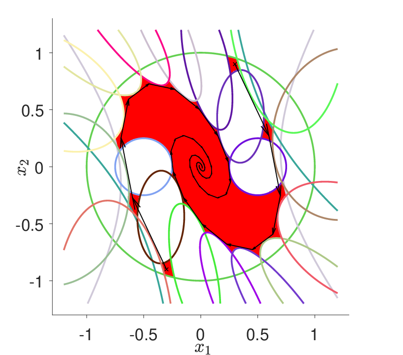
We consider the same dynamical system in Example 5.14 with additional quadratic constraints. Let the quadratic constraint set be . Note that there are quadratic constraints and that this set is nonconvex. Again, we use Algorithm 1 to compute the maximal CA-invariant set and it terminates at . The set is shown in Figure 2. Trajectories are also shown to verify set invariance of the disconnected regions.
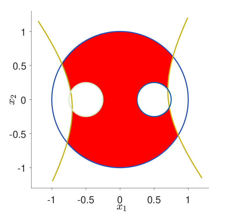
Additionaly, we also consider a nonlinear constraint, which is beyond the class of constraints that the approach in (Athanasopoulos and Jungers 2016) is able to handle. Let . It is easy to verify that Assumption 3 is satisfied with and . Using Algorithm 2, the maximal CA-invariant set can be obtained with as shown in Figure 3.


Example 5.15.
We consider an autonomous Wiener system, which consists of a linear dynamical system and a nonlinear static system (see (Markovsky 2019) for details on autonomous Wiener systems), as shown in Figure 4, with , and . The constraints are given by: and .
The output can be rewritten as
with
. The lifted system in (89) becomes
With the inequality , it can be easily verified that
Then, the constraint set for the lifted system is Finally, the lifted maximal CA-invariant set can be obtained using Algorithm 1, which terminates at . According to Proposition 3.10, the maximal CA-invariant set of the original system can be given by , which is shown in Figure 5. Again, a trajectory is given to verify set invariance of the disconnected regions.


Example 5.16.
Now, we evaluate the proposed approach on switched linear systems of different sizes. As we have already seen in Example 5.14, compared with the lifting approach in (Athanasopoulos and Jungers 2016), our approach takes fewer iterations for the same setting. In this example, we will make more comparison experiments in more difficult situations. Consider a switched linear system (93) with , which are randomly generated. To make sure that is satisfied, we first generate matrices and whose elements are sampled independently and identically from the uniform distribution between and . Then, we compute the JSR (or an upper bound) using the JSR toolbox (Vankeerberghen et al. 2014). Finally, we let
where . With this choice of , the condition that is satisfied for any . In the simulation, we set . The constraint set is given by , where the symmetric matrices and the vectors are also randomly generated. We then use Algorithm 1 with the modifications in (95)-(96) and (99)-(100) to compute . Let denote the number of iterations and denote the number of constraints in the expression of (or equivalently ) after removing redundancy by solving (49). Note that different approaches may result in different descriptions of in the presence of nonlinear constraints though the set is fixed, because identifying redundant nonlinear constraints requires us to solve non-convex problems, see Problems (14) and (15). The comparison with the lifting approach in (Athanasopoulos and Jungers 2016) is made in terms of the number of iterations and the number of constraints in the expression of . Similarly, let and denote the number of iterations and the number of constraints respectively in (Athanasopoulos and Jungers 2016). The approach in (Athanasopoulos and Jungers 2016) lifts the system into a -dimensional system, where the quadratic constraints become linear constraints, while our approach does not have to lift the system as the constraints are quadratic. For the lifted system of (Athanasopoulos and Jungers 2016), all the sets from (9) are polyhedra and we can remove redundancy by solving linear optimization problems according to the extended Farkas’ lemma (Schrijver 1986; Blanchini 1999). The computation of polyhedra is implemented with the Multi-Parametric Toolbox (Herceg et al. 2013), which allows to remove redundancy efficiently.
We take realizations of the dynamics and the constraints and compute the mean values of , , and , denoted by , , , and respectively. The results are shown in Table 1. When , the approach in (Athanasopoulos and Jungers 2016) is not conducted as it takes too much time. As we can see in Table 1, the proposed approach converges faster and produces a tighter expression of with a smaller number of constraints.
| - | - | |||
| - | - | |||
| - | - | |||
| - | - |
Example 5.17.
In the rest of this section, we consider the following nonlinear system
| (123) |
The state constraint set is given by . There exists a diffeomorphism ,
such that the nonlinear system can be linearized into
With the state transformation , the state constraint set of the linearized system can be given by . As a result, we get a linear system with quadratic constraints and the constraint set is bounded. Using Algorithm 1, the maximal CA-invariant set of the linearized system can be computed and it takes iterations. The set is shown in Figure 6.


Using the inverse mapping ,
the maximal CA-invariant set of the original nonlinear system can be obtained and is shown in Figure 7.


6 Conclusions
We have studied the computation of the maximal CA-invariant set of discrete-time linear systems subject to a class of non-convex constraints that admit quadratic lower and upper bounds. By the use of these quadratic bounds, we have derived a sufficient condition for set invariance, which can be expressed as a set of LMIs. Based on this sufficient condition, a new algorithm is presented by solving a number of convex problems with only one LMI constraint at every iteration. Under mild assumptions, finite convergence to the exact maximal CA-invariant set can be guaranteed. This algorithm can be extended to switched linear systems and some special nonlinear systems that admit linear equivalents. To illustrate the performance of the proposed algorithm, we have presented several numerical examples and made comparison with an existing approach, which is capable of computing the exact maximal CA-invariant set of switched linear systems subject to semi-algebraic constraints. For the same setting, we show that our approach converges faster with a tighter expression of the maximal CA-invariant set.
Appendix
Proof of Proposition 3.5
In the case of linear constraints, is a polyhedral set for any . It is clear from Lemma 1 that implies . We only need to show implies . From (10), if and only if . From the extended Farkas’ lemma (Schrijver 1986; Blanchini 1999), for any , if and only if there exists a non-negative matrix such that,
| (134) |
Suppose there exists a non-negative matrix satisfying (Proof of Proposition ) and (134) for some , by simple manipulations, we can see that and for any , which implies that
This means that for any . Hence, .
References
- (1)
- Ahmadi and Gunluk (2018) Ahmadi, A. A. and Gunluk, O. (2018). Robust-to-dynamics optimization, arXiv preprint arXiv:1805.03682 .
- Alamo et al. (2009) Alamo, T., Cepeda, A., Fiacchini, M. and Camacho, E. F. (2009). Convex invariant sets for discrete-time lur’e systems, Automatica 45(4): 1066–1071.
- Artstein and Raković (2008) Artstein, Z. and Raković, S. V. (2008). Feedback and invariance under uncertainty via set-iterates, Automatica 44(2): 520–525.
- Athanasopoulos and Jungers (2016) Athanasopoulos, N. and Jungers, R. M. (2016). Computing the domain of attraction of switching systems subject to non-convex constraints, Proceedings of the 19th International Conference on Hybrid Systems: Computation and Control, ACM, pp. 41–50.
- Athanasopoulos and Jungers (2018) Athanasopoulos, N. and Jungers, R. M. (2018). Combinatorial methods for invariance and safety of hybrid systems, Automatica 98: 130–140.
- Athanasopoulos et al. (2017) Athanasopoulos, N., Smpoukis, K. and Jungers, R. M. (2017). Invariant sets analysis for constrained switching systems, IEEE Control Systems Letters 1(2): 256–261.
- Aubin (1991) Aubin, J. P. (1991). Viability theory., Basel: Birkhauser.
- Aubin (2009) Aubin, J. P. (2009). Viability theory, Springer Science & Business Media.
- Belta et al. (2017) Belta, C., Yordanov, B. and Gol, E. A. (2017). Formal Methods for Discrete-Time Dynamical Systems, Vol. 89, Springer.
- Bertsekas (2009) Bertsekas, D. P. (2009). Convex optimization theory, Athena Scientific.
- Blanchini (1999) Blanchini, F. (1999). Set invariance in control, Automatica 35(11): 1747–1767.
- Blanchini and Miani (2008) Blanchini, F. and Miani, S. (2008). Set-Theoretic Methods in Control, Birkhauser.
- Blondel and Nesterov (2005) Blondel, V. D. and Nesterov, Y. (2005). Computationally efficient approximations of the joint spectral radius, SIAM Journal on Matrix Analysis and Applications 27(1): 256–272.
- Boyd et al. (1994) Boyd, S., El Ghaoui, L., Feron, E. and Balakrishnan, V. (1994). Linear Matrix Inequalities in System and Control Theory, Society for Industrial and Applied Mathematics (SIAM).
- Bravo et al. (2005) Bravo, J. M., Limón, D., Alamo, T. and Camacho, E. F. (2005). On the computation of invariant sets for constrained nonlinear systems: An interval arithmetic approach, Automatica 41(9): 1583–1589.
- Darup and Cannon (2017) Darup, M. S. and Cannon, M. (2017). On the computation of -contractive sets for linear constrained systems, IEEE Transactions on Automatic Control 62(3): 1498–1504.
- Dehghan and Ong (2012a) Dehghan, M. and Ong, C. (2012a). Discrete-time switching linear system with constraints: Characterization and computation of invariant sets under dwell-time consideration, Automatica 5(48): 964–969.
- Dehghan and Ong (2012b) Dehghan, M. and Ong, C. J. (2012b). Characterization and computation of disturbance invariant sets for constrained switched linear systems with dwell time restriction, Automatica 48(9): 2175–2181.
- Derinkuyu and Pınar (2006) Derinkuyu, K. and Pınar, M. (2006). On the S-procedure and some variants, Mathematical Methods of Operations Research 64(1): 55–77.
- Dorea and Hennet (1999) Dorea, C. E. T. and Hennet, J. C. (1999). (A, B)-invariant polyhedral sets of linear discrete-time systems, Journal of Optimization Theory and Applications 103(3): 521–542.
- Fiacchini et al. (2010) Fiacchini, M., Alamo, T. and Camacho, E. F. (2010). On the computation of convex robust control invariant sets for nonlinear systems, Automatica 46(8): 1334–1338.
- Gilbert et al. (1995) Gilbert, E. G., Kolmanovsky, I. and Tan, K. T. (1995). Discrete-time reference governors and the nonlinear control of systems with state and control constraints, International Journal of Robust and Nonlinear Control 5: 487–504.
- Gilbert and Tan (1991) Gilbert, E. G. and Tan, K. T. (1991). Linear systems with state and control constraints: The theory and application of maximal output admissible sets, IEEE Transactions on Automatic Control 36: 1008–1020.
- Gutman and Cwikel (1987) Gutman, P. O. and Cwikel, M. (1987). An algorithm to find maximal state constraint sets for discrete-time linear dynamical systems with bounded controls and states, IEEE Transactions on Automatic Control 32(3): 251–254.
- Henrion and Korda (2014) Henrion, D. and Korda, M. (2014). Convex computation of the region of attraction of polynomial control systems, IEEE Transactions on Automatic Control 59(2): 297–312.
- Herceg et al. (2013) Herceg, M., Kvasnica, M., Jones, C. and Morari, M. (2013). Multi-Parametric Toolbox 3.0, Proceedings of the European Control Conference, Zürich, Switzerland, pp. 502–510. http://control.ee.ethz.ch/~mpt.
- Hernández-Mejías et al. (2016) Hernández-Mejías, M. A., Sala, A., Ariño, C. and Querol, A. (2016). Reliable controllable sets for constrained markov-jump linear systems, International Journal of Robust and Nonlinear Control 26(10): 2075–2089.
- Jungers (2009) Jungers, R. M. (2009). The joint spectral radius: theory and applications, Vol. 385, Springer Science & Business Media.
- Jungers and Tabuada (2019) Jungers, R. M. and Tabuada, P. (2019). Non-local linearization of nonlinear differential equations via polyflows, Proceedings of the American Control Conference, pp. 1–6.
- Kolmanovsky and Gilbert (1998) Kolmanovsky, I. and Gilbert, E. G. (1998). Theory and computation of disturbance invariant sets for discrete-time linear systems, Mathematical Problems in Engineering 4: 317–367.
- Korda et al. (2014) Korda, M., Henrion, D. and Jones, C. N. (2014). Convex computation of the maximum controlled invariant set for polynomial control systems, SIAM Journal on Control and Optimization 52(5): 2944–2969.
- Legat et al. (2018) Legat, B., Tabuada, P. and Jungers, R. M. (2018). Computing controlled invariant sets for hybrid systems with applications to model-predictive control, IFAC-PapersOnLine 51(16): 193–198.
- Levine and Marino (1986) Levine, J. and Marino, R. (1986). Nonlinear system immersion, observers and finite-dimensional filters, Systems & Control Letters 7(2): 133–142.
- Markovsky (2019) Markovsky, I. (2019). On the behavior of autonomous wiener systems, Automatica 110: 108601.
- Mayne et al. (2000) Mayne, D. Q., Rawlings, J. B., Rao, C. V. and Scokaert, P. O. M. (2000). Constrained model predictive control: Stability and optimality, Automatica 36(6): 789–814.
- Menini and Tornambè (2012) Menini, L. and Tornambè, A. (2012). Exact and approximate feedback linearization without the linear controllability assumption, Automatica 48(9): 2221–2228.
- Necoara et al. (2019) Necoara, I., Nesterov, Y. and Glineur, F. (2019). Linear convergence of first order methods for non-strongly convex optimization, Mathematical Programming 175(1-2): 69–107.
- Ong and Gilbert (2006) Ong, C. J. and Gilbert, E. G. (2006). The minimal disturbance invariant set: Outer approximations via its partial sums, Automatica 42(9): 1563–1568.
- Parrilo (2003) Parrilo, P. A. (2003). Semidefinite programming relaxations for semialgebraic problems, Mathematical programming 96(2): 293–320.
- Pluymers et al. (2005) Pluymers, B., Rossiter, J. A., Suykens, J. A. K. and De Moor, B. (2005). The efficient computation of polyhedral invariant sets for linear systems with polytopic uncertainty, Proceedings of the American Control Conference, pp. 804–809.
- Powers and Wörmann (1998) Powers, V. and Wörmann, T. (1998). An algorithm for sums of squares of real polynomials, Journal of pure and applied algebra 127(1): 99–104.
- Rakovic et al. (2005) Rakovic, S. V., Kerrigan, E. C., Kouramas, K. I. and Mayne, D. Q. (2005). Invariant approximations of the minimal robust positively invariant set, IEEE Transactions on Automatic Control 50(3): 406–410.
- Raković et al. (2007) Raković, S. V., Kerrigan, E. C., Mayne, D. Q. and Kouramas, K. I. (2007). Optimized robust control invariance for linear discrete-time systems: Theoretical foundations, Automatica 43(5): 831–841.
- Rungger and Tabuada (2017) Rungger, M. and Tabuada, P. (2017). Computing robust controlled invariant sets of linear systems, IEEE Transactions on Automatic Control 62(7): 3665–3670.
- Sassi and Girard (2012) Sassi, M. A. B. and Girard, A. (2012). Computation of polytopic invariants for polynomial dynamical systems using linear programming, Automatica 48(12): 3114–3121.
- Schrijver (1986) Schrijver, A. (1986). Theory of linear and integer programming, John Wiley & Sons.
- Su (1982) Su, R. (1982). On the linear equivalents of nonlinear systems, Systems & Control Letters 2(1): 48–52.
- Trodden (2016) Trodden, P. (2016). A one-step approach to computing a polytopic robust positively invariant set, IEEE Transactions on Automatic Control 61(12): 4100–4105.
- Vankeerberghen et al. (2014) Vankeerberghen, G., Hendrickx, J. and Jungers, R. M. (2014). Jsr: A toolbox to compute the joint spectral radius, Proceedings of the 17th international conference on Hybrid systems: computation and control, ACM, pp. 151–156.
- Wang et al. (2019) Wang, Z., Jungers, R. M. and Ong, C. J. (2019). Computation of the maximal invariant set of linear systems with quasi-smooth nonlinear constraints, Proceedings of the European Control Conference, pp. 3803–3808.
- Wang et al. (2020) Wang, Z., Jungers, R. M. and Ong, C. J. (2020). Computing invariant sets of discrete-time nonlinear systems via state immersion, The 21st IFAC World Congress, Berlin, Germany, pp. 5579–5584.