跳到论文正文
W Papers独立论文阅读器 arXiv:1912.09627 论文正文 计算阅读时间 · 0%
引用这篇论文根据当前论文元数据生成,正式投稿前建议核对。


License: CC BY-NC-SA 4.0
arXiv:1912.09627v1 [math.NA] 20 Dec 2019

The Virtual Element Method
for a Minimal Surface Problem

P. F. Antonietti Affiliation:  MOX, Dipartimento di Matematica, Politecnico di Milano, Italy; e-mail: paola.antonietti@polimi.it    S. Bertoluzza Affiliation: Istituto di Matematica Applicata e Tecnologie Informatiche - CNR, Pavia, Italy e-mail: silvia.bertoluzza@imati.cnr.it    D. Prada Affiliation: Istituto di Matematica Applicata e Tecnologie Informatiche - CNR, Pavia, Italy e-mail: daniele.prada@imati.cnr.it    M. Verani Affiliation:  MOX, Dipartimento di Matematica, Politecnico di Milano, Italy and Istituto di Matematica Applicata e Tecnologie Informatiche - CNR, Pavia, Italy e-mail: marco.verani@polimi.it
Abstract

In this paper we consider the Virtual Element discretization of a minimal surface problem, a quasi-linear elliptic partial differential equation modeling the problem of minimizing the area of a surface subject to a prescribed boundary condition. We derive optimal error estimate and present several numerical tests assessing the validity of the theoretical results.

1 Introduction

In recent years, the numerical approximation of partial differential equations on computational meshes composed by arbitrarily-shaped polygonal/polyhedral (polytopal, for short) elements has been the subject of an intense research activity. Examples of such methods include the Mimetic Finite Difference method, the Polygonal Finite Element Method, the polygonal Discontinuous Galerkin Finite Element Methods, the Hybridizable Discontinuous Galerkin and Hybrid High-Order Methods, the Gradient Discretization method, the Finite Volume Method, the BEM-based FEM, the Weak Galerkin method and the Virtual Element method (VEM). For more details see the special issue [6] and the references therein. VEM has been introduced in [10] for elliptic problems and later extended to several different linear and non-linear differential problems. While the analysis of linear problems is much more flourished, the study of Virtual Element discretization for non-linear problems is much less developed (see, e.g., [4, 15, 11, 9, 5, 7, 12, 20, 3, 2, 1, 17]). In this paper we contribute to fill this gap by addressing the (lowest order) Virtual Element discretization of a minimal surface problem (see, e.g., [13] for its finite element discretization). More precisely, in Section 2 we introduce the continuous problem together with its Virtual Element discretization, while in Section 3 we derive optimal error estimate in the H1H^{1}-norm, under a condition on the discrete solution, the validity of which can be checked “a posteriori”. Finally, in Section 4 we present several numerical results assessing the validity of the theoretical estimate and confirming that optimal convergence is indeed achieved. Moreover, the convergence properties in the L2L^{2}-norm is numerically investigated.

1.1 Notation

Throughout the paper we shall use the standard notation of the Sobolev spaces Hm​(𝒟)H^{m}(\mathcal{D}) for a nonnegative integer mm and an open bounded domain 𝒟\mathcal{D}. The mm-th seminorm of the function vv will be denoted by

|v|2m,𝒟=∑|α|=m∥∂|α|v∂x1α1∂x2α2∥20,𝒟,|v|{{}^{2}}_{m,\mathcal{D}}=\sum_{|\alpha|=m}\bigg\|\frac{\partial^{|\alpha|}v}{\partial_{x_{1}}^{\alpha_{1}}\partial_{x_{2}}^{\alpha_{2}}}\bigg\|^{2}_{0,\mathcal{D}},

where ∥⋅∥0,𝒟\|\cdot\|_{0,\mathcal{D}} stands for the L2​(𝒟)L^{2}(\mathcal{D}) norm and we set |α|=α1+α2|{\alpha}|=\alpha_{1}+\alpha_{2} for the nonnegative multi-index α=(α1,α2){\alpha}=(\alpha_{1},\alpha_{2}). For any integer m≥0m\geq 0, ℙm​(𝒟)\mathbb{P}^{m}({\mathcal{D}}) is the space of polynomials of total degree up to mm defined on 𝒟{\mathcal{D}}. Moreover, n=(n1,n2)n=(n_{1},n_{2}) is the outward unit normal vector to ∂𝒟\partial\mathcal{D}, the boundary of 𝒟\mathcal{D}. Finally, we will employ the symbol ≲\lesssim for an inequality holding up to a constant independent of the mesh size.

2 Continuous problem and its VEM discretization

Let Ω⊆ℝ2\Omega\subseteq\mathbb{R}^{2} be a bounded open set. In the following, we will employ the following notation

f⁡(⋅)=1+|∇(⋅)|2.f(\cdot)=\sqrt{1+|\nabla(\cdot)|^{2}}.

Let φ\varphi be a function given on the boundary Γ=∂Ω\Gamma=\partial\Omega. The minimal surface problem amounts to finding a function uu which minimizes the functional

J⁡(v)=∫Ωf⁡(v)​𝑑xJ(v)=\int_{\Omega}f(v)dx

over a suitable space of functions which are equal to φ\varphi on Γ\Gamma. The existence and uniqueness of a solution is a delicate mathematical issue (see, e.g., [13] and the references therein). Here, with the aim of simplifying the analysis, we follow the framework considered, e.g., in [13] and make the following hypotheses: the domain Ω\Omega is a convex polygonal set and the function φ\varphi is the trace over Γ\Gamma of a function (by abuse of notation still denoted by φ\varphi) of H2​(Ω)H^{2}(\Omega). Moreover, for the subsequent discussion, as in [13], we consider that the minimal surface problem consists in solving the following:

u=arg​minv∈Vφ⁡J⁡(v),u=\mathop{\mathrm{arg\,min}}_{v\in V^{\varphi}}J(v), (1)

where Vφ={v∈H1​(Ω):u=φ​ on ​∂Ω}V^{\varphi}=\{v\in H^{1}(\Omega):~u=\varphi\text{~on~}\partial\Omega\}. Note that uu is the solution to (1) if and only if u∈Vφu\in V^{\varphi} solves

∫Ω∇u⋅∇vf⁡(u)=0∀v∈V0=H01​(Ω).\int_{\Omega}\frac{\nabla u\cdot\nabla v}{f(u)}=0\qquad\forall v\in V^{0}=H^{1}_{0}(\Omega). (2)

Let {𝒯h}h\{\mathcal{T}_{h}\}_{h} be a sequence of decompositions (meshes) of Ω\Omega into non-overlapping polygons EE. Each mesh 𝒯h\mathcal{T}_{h} is labeled by the mesh size parameter hh, which will be defined below, and satisfies suitable regularity assumptions that are customarily made to prove the convergence of the method and derive an estimate of the approximation error. These regularity assumptions are introduced and discussed in Section 3. Let ℰh\mathcal{E}_{h} be the set of edges of 𝒯h\mathcal{T}_{h} such that ℰh=ℰhi∪ℰhΓ\mathcal{E}_{h}=\mathcal{E}_{h}^{i}\cup\mathcal{E}_{h}^{\Gamma}, where ℰhi\mathcal{E}_{h}^{i} and ℰhΓ\mathcal{E}_{h}^{\Gamma} are the set of interior and boundary edges, respectively. Similarly, we denote by Vh=Vhi∪VhΓV_{h}=V_{h}^{i}\cup V_{h}^{\Gamma} the set of vertices in 𝒯h\mathcal{T}_{h}, where VhiV_{h}^{i} and VhΓV_{h}^{\Gamma} are the sets of interior and boundary vertices, respectively. Accordingly, VhEV_{h}^{E} is the set of vertices of EE. Moreover, |E||E| and |e||e| denote the area of cell EE and the length of edge ee, respectively, ∂E\partial E is the boundary of EE, hEh_{E} is the diameter of EE and the mesh size parameter is defined as h=maxE∈𝒯h⁡hEh=\max_{E\in\mathcal{T}_{h}}h_{E}.

Let us introduce the usual local lowest order conforming Virtual Element space on the polygon EE (see, e.g., [10])

VhE={vh∈H1(E):Δvh=0 in E,vh∈C0(∂E),vh|e∈ℙ1(e)∀e∈∂E},V^{E}_{h}=\{v_{h}\in H^{1}(E):~\Delta v_{h}=0\text{~in~}E,~v_{h}\in C^{0}(\partial E),v_{h}|_{e}\in\mathbb{P}^{1}(e)~\forall e\in\partial E\},

where, for DD dd-dimensional domain, ℙ1​(D)\mathbb{P}^{1}(D) denotes the space of dd-variate polynomials of order less than or equal to one on DD. Accordingly, the global Virtual Element space is defined as follows

Vhφ={vh∈H1(Ω):vh|E∈VhE,vh(V)=φ(V) for each vertex V∈VhΓ}.V_{h}^{\varphi}=\{v_{h}\in H^{1}(\Omega):~v_{h}|_{E}\in V_{h}^{E},~v_{h}(V)=\varphi(V)~\text{~for~each~vertex~V}\in V_{h}^{\Gamma}\}.

Consistently, we denote by Vh0V_{h}^{0} the global VEM space with homogeneous Dirichlet boundary conditions.

Let SE​(⋅,⋅)S^{E}(\cdot,\cdot) be the usual stabilization term employed for constructing the VEM discretization of the Laplace problem, i.e. the Euclidean scalar product associated with the degrees of freedom (here the vertex values). See, e.g., [10, 8] for further details. Moreover, let ΠE∇:VhE→ℙ1​(E)\Pi^{\nabla}_{E}\colon V^{E}_{h}\rightarrow\mathbb{P}^{1}(E) the usual elliptic projection operator (see, e.g., [10]).

We introduce the local discrete function fhE:VhE→ℝf^{E}_{h}:V^{E}_{h}\to\mathbb{R} defined as

fhE​(vh)=1+|∇Π∇Evh|2+|E|−1SE((I−Π∇E)vh,(I−Π∇E)vh).f^{E}_{h}(v_{h})=\sqrt{1+|\nabla\Pi^{\nabla}_{E}v_{h}|^{2}+|E|^{-1}S^{E}((I-\Pi^{\nabla}_{E})v_{h},(I-\Pi^{\nabla}_{E})v_{h})}. (3)

Roughly speaking, fhE​(⋅)f_{h}^{E}(\cdot) represents an approximation to 1+|(∇⋅)|E|2\sqrt{1+|(\nabla\cdot)_{|E}|^{2}}.

Having in mind the above definitions, the discrete virtual counterpart of the continuous minimization problem (1) reads as follows

uh=arg​minvh∈Vhφ⁡Jh​(vh), with Jh​(vh)=∑E∈𝒯h∫EfhE​(vh)​𝑑x.u_{h}=\mathop{\mathrm{arg\,min}}_{v_{h}\in V_{h}^{\varphi}}J_{h}(v_{h}),\quad\text{ with }\quad J_{h}(v_{h})=\sum_{E\in\mathcal{T}_{h}}\int_{E}f^{E}_{h}(v_{h})\,dx. (4)

Thus, the Virtual Element discretization of (2) is as follows: find uh∈Vhφu_{h}\in V_{h}^{\varphi} such that

Ah​(uh,uh,vh)=0A_{h}(u_{h};u_{h},v_{h})=0 (5)

for all vh∈Vh0v_{h}\in V_{h}^{0}, where Ah​(wh,uh,vh)=∑EAhE​(wh,uh,vh)A_{h}(w_{h};u_{h},v_{h})=\sum_{E}A_{h}^{E}(w_{h};u_{h},v_{h}) and

AhE​(wh,uh,vh)=∫E∇Π∇Euh⋅∇Π∇EvhfhE​(wh)​𝑑x+SE​((I−ΠE∇)​uh,(I−ΠE∇)​vh)fhE​(wh).A_{h}^{E}(w_{h};u_{h},v_{h})=\int_{E}\frac{\nabla\Pi^{\nabla}_{E}u_{h}\cdot\nabla\Pi^{\nabla}_{E}v_{h}}{f^{E}_{h}(w_{h})}\,dx+\frac{S^{E}((I-\Pi^{\nabla}_{E})u_{h},(I-\Pi^{\nabla}_{E})v_{h})}{f^{E}_{h}(w_{h})}. (6)

Note that as fhE​(wh)f_{h}^{E}(w_{h}) is constant on each polygon EE, the form AhE​(⋅,⋅,⋅)A^{E}_{h}(\cdot;\cdot,\cdot) can be equivalently written as

AhE​(wh,uh,vh)=ahE​(uh,vh)fhE​(wh)A_{h}^{E}(w_{h};u_{h},v_{h})=\frac{a_{h}^{E}(u_{h},v_{h})}{f_{h}^{E}(w_{h})} (7)

where

ahE(uh,vh)=∫E∇ΠE∇uh⋅∇ΠE∇vhdx+SE((I−ΠE∇)uh,(I−ΠE∇)vh)a_{h}^{E}(u_{h},v_{h})=\int_{E}\nabla\Pi^{\nabla}_{E}u_{h}\cdot\nabla\Pi^{\nabla}_{E}v_{h}dx+S^{E}((I-\Pi^{\nabla}_{E})u_{h},(I-\Pi^{\nabla}_{E})v_{h})

is the classical local discrete VEM bilinear form for the Laplace problem. It is worth remembering (see, e.g., [10]) that ahE​(⋅,⋅)a_{h}^{E}(\cdot,\cdot) satisfies the following two crucial properties:

(i)(i)

Consistency: for every polynomial q∈ℙ1​(E)q\in\mathbb{P}^{1}(E) and function vh∈VhEv_{h}\in V_{h}^{E} we have:

ahE​(vh,q)=aE​(vh,q);\displaystyle a^{E}_{h}(v_{h},q)=a^{E}(v_{h},q); (8)
(i​i)(ii)

Stability: there exist two positive constants α∗\alpha_{*}, α∗\alpha^{*} independent of hh and EE such that for every vh∈VhEv_{h}\in V_{h}^{E} it holds:

α∗​aE​(vh,vh)≤ahE​(vh,vh)≤α∗​aE​(vh,vh).\displaystyle\alpha_{*}a^{E}(v_{h},v_{h})\leq a^{E}_{h}(v_{h},v_{h})\leq\alpha^{*}a^{E}(v_{h},v_{h}). (9)

Remark that requiring that the stability condition (i​i)(ii) holds is equivalent to requiring that there exists positive constants α~∗\widetilde{\alpha}_{*} and α~∗\widetilde{\alpha}^{*} such that, for all vh∈VhEv_{h}\in V_{h}^{E} with ΠE∇​vh=0\Pi^{\nabla}_{E}v_{h}=0 it holds:

α~∗​aE​(vh,vh)≤SE​(vh,vh)≤α~∗​aE​(vh,vh),\displaystyle{\widetilde{\alpha}}_{*}a^{E}(v_{h},v_{h})\leq S^{E}(v_{h},v_{h})\leq{\widetilde{\alpha}}^{*}a^{E}(v_{h},v_{h}), (10)

(see [10] for more details). Existence and uniqueness of the solution uh∈Vhφu_{h}\in V_{h}^{\varphi} follow by working on the discrete cost functional Jh​(vh)J_{h}(v_{h}) as in [13].

For future use, we set aE​(uh,vh)=∫E∇uh⋅∇vh​𝑑xa^{E}(u_{h},v_{h})=\int_{E}\nabla u_{h}\cdot\nabla v_{h}dx.

3 Error analysis

We make the following regularity assumptions on the mesh sequence {𝒯h}h\{\mathcal{T}_{h}\}_{h}:

  • (H)

    there exists a constant ρ0>0\rho_{0}>0 independent of 𝒯h\mathcal{T}_{h}, such that for every element EE it holds:

    1. (H1)

      EE is star-shaped with respect to all the points of a ball of radius ρ0​hE\rho_{0}h_{E}

    2. (H2)

      every edge e∈ℰhe\in\mathcal{E}_{h} has length |e|≥ρ0​hE|e|\geq\rho_{0}h_{E}.

The assumptions (H1)-(H2) are standard (see, e.g.,  [10]) and allow to define, for every smooth enough function vv, an “interpolant” vIv_{I} in VhφV^{\varphi}_{h} such that it holds |v−vI|1,Ω≲h|v-v_{I}|_{{1,\Omega}}{\lesssim}h (see [10]).

We now state the main result of the paper.

Theorem 3.1.

Let u∈H2​(Ω)∩W1,∞​(Ω)u\in H^{2}(\Omega)\cap W^{1,\infty}(\Omega) be the continuous solution to (1), and let uh∈Vhφu_{h}\in V_{h}^{\varphi} be the VEM solution to (5). Letting

C⁡(uh)=h−1​∑ESE​((I−ΠE∇)​uh,(I−ΠE∇)​uh),C(u_{h})=h^{-1}\sqrt{\sum_{E}S^{E}((I-\Pi_{E}^{\nabla})u_{h},(I-\Pi_{E}^{\nabla})u_{h}),}

it holds

|u−uh|1,Ω≲(1+C⁡(uh))2​h.|u-u_{h}|_{{1,\Omega}}\lesssim(1+C(u_{h}))^{2}h. (11)
Corollary 3.2.

Assume that C⁡(uh)≲1C(u_{h})\lesssim 1. Then it holds that

|u−uh|1,Ω≲h.|u-u_{h}|_{{1,\Omega}}\lesssim h.
Proof.

By triangle inequality we have

|u−uh|1,Ω≤|u−uI|1,Ω+|​uI−uh|1,Ω.|u-u_{h}|_{{1,\Omega}}\leq|u-u_{I}|_{{1,\Omega}}+|u_{I}-u_{h}|_{{1,\Omega}}.

In the following, we adapt the ideas of [16] to the present context. We preliminary observe that the following holds true

|uI−uh|1,Ω\displaystyle|u_{I}-u_{h}|_{{1,\Omega}} =\displaystyle= (∑E∈𝒯h∫E|∇(uI−uh)|2fhE​(uh)​fhE​(uh))1/2\displaystyle\left(\sum_{E\in\mathcal{T}_{h}}\int_{E}\frac{|\nabla(u_{I}-u_{h})|^{2}}{f_{h}^{E}(u_{h})}f^{E}_{h}(u_{h})\right)^{1/2} (12)
≤\displaystyle\leq (maxE⁡|fhE​(uh)|)1/2​(∑E∈𝒯h∫E|∇(uI−uh)|2fhE​(uh))1/2.\displaystyle\left(\max_{E}|f^{E}_{h}(u_{h})|\right)^{1/2}\left(\sum_{E\in\mathcal{T}_{h}}\int_{E}\frac{|\nabla(u_{I}-u_{h})|^{2}}{f^{E}_{h}(u_{h})}\right)^{1/2}.

The remaining part of the proof is devoted to show:

  • (i)

    (∑E∈𝒯h∫E|∇(uI−uh)|2fhE​(uh))1/2≲(1+C⁡(uh))​h\displaystyle{\left(\sum_{E\in\mathcal{T}_{h}}\int_{E}\frac{|\nabla(u_{I}-u_{h})|^{2}}{f_{h}^{E}(u_{h})}\right)^{1/2}\lesssim(1+C(u_{h}))h};

  • (ii)

    maxE⁡|fhE​(uh)|≲(1+C⁡(uh))2\displaystyle{\max_{E}|f^{E}_{h}(u_{h}){|}\lesssim(1+C(u_{h}))^{2}}.

Let us first prove (i)(i). We start by observing that, thanks to (10), we have

|uh−ΠE∇​uh|1,h≲C⁡(uh)​h|u_{h}-\Pi^{\nabla}_{E}u_{h}|_{1,h}\lesssim C(u_{h})h (13)

where where |v|1,h2=∑E∈𝒯h‖∇v‖0,E2|v|_{1,h}^{2}=\sum_{E\in\mathcal{T}_{h}}{\|\nabla v\|_{0,E}^{2}}. By using the stability property of ahE​(⋅,⋅)a_{h}^{E}(\cdot,\cdot), as fhE​(uh)f_{h}^{E}(u_{h}) is constant on EE, we get the following inequalities with δh=uh−uI\delta_{h}=u_{h}-u_{I}

∑E∈𝒯h∫E|∇(uI−uh)|2fhE​(uh)\displaystyle\sum_{E\in\mathcal{T}_{h}}\int_{E}\frac{|\nabla(u_{I}-u_{h})|^{2}}{f_{h}^{E}(u_{h})} ≲\displaystyle\lesssim ∑E∈𝒯hahE​(δh,δh)fhE​(uh)\displaystyle\sum_{E\in\mathcal{T}_{h}}\frac{a_{h}^{E}(\delta_{h},\delta_{h})}{f_{h}^{E}(u_{h})} (14)
≲\displaystyle\lesssim |−∑E∈𝒯hahE​(uI,δh)fhE​(uh)|,\displaystyle\left|-\sum_{E\in\mathcal{T}_{h}}\frac{a_{h}^{E}(u_{I},\delta_{h})}{f_{h}^{E}(u_{h})}\right|,

where in the last step we employ (5) with δh∈Vh0\delta_{h}\in V_{h}^{0}. Let uπ|Eu_{\pi}|_{E} be the L2​(E)L^{2}(E) projection of uu onto ℙ1​(E)\mathbb{P}^{1}(E). By employing the consistency and stability properties of ahE​(⋅,⋅)a_{h}^{E}(\cdot,\cdot) together with the fact that uu is solution to (1), it is immediate to check that the following holds

−∑E∈𝒯hahE​(uI,δh)fhE​(uh)\displaystyle-\sum_{E\in\mathcal{T}_{h}}\frac{a_{h}^{E}(u_{I},\delta_{h})}{f^{E}_{h}(u_{h})} =\displaystyle= −∑E∈𝒯h{ahE​(uI−uπ,δh)fhE​(uh)+ahE​(uπ,δh)fhE​(uh)\displaystyle-\sum_{E\in\mathcal{T}_{h}}\Bigg\{\frac{a_{h}^{E}(u_{I}-u_{\pi},\delta_{h})}{f^{E}_{h}(u_{h})}+\frac{a_{h}^{E}(u_{\pi},\delta_{h})}{f^{E}_{h}(u_{h})} (15)
±aE​(u,δh)fhE​(uh)−∫E∇u⋅∇δhf⁡(u)dx}\displaystyle\pm\frac{a^{E}(u,\delta_{h})}{f^{E}_{h}(u_{h})}-\int_{E}\frac{\nabla u\cdot\nabla\delta_{h}}{f(u)}dx\Bigg\}
=\displaystyle= ∑E∈𝒯hahE​(uπ−uI,δh)fhE​(uh)+∑E∈𝒯haE​(u−uπ,δh)fhE​(uh)\displaystyle\sum_{E\in\mathcal{T}_{h}}\frac{a_{h}^{E}(u_{\pi}-u_{I},\delta_{h})}{f^{E}_{h}(u_{h})}+\sum_{E\in\mathcal{T}_{h}}\frac{a^{E}(u-u_{\pi},\delta_{h})}{f^{E}_{h}(u_{h})}
+∑E∈𝒯h∫E∇u⋅∇δh(1f⁡(u)−1fhE​(uh))dx\displaystyle+\sum_{E\in\mathcal{T}_{h}}\int_{E}\nabla u\cdot\nabla\delta_{h}\left(\frac{1}{f(u)}-\frac{1}{f^{E}_{h}(u_{h})}\right)dx
=\displaystyle= A+B+C.\displaystyle A+B+C. (16)

We now bound the three terms separately. By combining the Cauchy-Schwarz inequality with the fact that fhE​(uh)f_{h}^{E}(u_{h}) is constant and larger than 11 on each polygon EE, we have

A≤(|u−uπ|1,h+|​u−uI|1,Ω)​(∑E∈𝒯h∫E|∇(uI−uh)|2fhE​(uh)​𝑑x)1/2,\displaystyle A\leq(|u-u_{\pi}|_{1,h}+|u-u_{I}|_{{1,\Omega}})\left(\sum_{E\in\mathcal{T}_{h}}\int_{E}\frac{|\nabla(u_{I}-u_{h})|^{2}}{f^{E}_{h}(u_{h})}dx\right)^{1/2}, (17)

and

B≤|u−uπ|1,h​(∑E∈𝒯h∫E|∇(uI−uh)|2fhE​(uh)​𝑑x)1/2.\displaystyle B\leq|u-u_{\pi}|_{1,h}\left(\sum_{E\in\mathcal{T}_{h}}\int_{E}\frac{|\nabla(u_{I}-u_{h})|^{2}}{f^{E}_{h}(u_{h})}dx\right)^{1/2}. (18)

Finally, setting γ=maxΩ¯⁡|∇u|f⁡(u)\gamma=\max_{\bar{\Omega}}\frac{|\nabla u|}{f(u)}, employing the definitions of f⁡(⋅)f(\cdot) and fhE​(⋅)f^{E}_{h}(\cdot) and observing that f⁡(u)≥|∇u|f(u)\geq|\nabla u|, the following holds

C\displaystyle C =\displaystyle= ∑E∈𝒯h∫E∇u⋅∇δh[fhE​(uh)]2−f2​(u)f⁡(u)​fhE​(uh)​(f⁡(u)+fhE​(uh))dx\displaystyle\sum_{E\in\mathcal{T}_{h}}\int_{E}\nabla u\cdot\nabla\delta_{h}\frac{[f_{h}^{E}(u_{h})]^{2}-f^{2}(u)}{f(u)f_{h}^{E}(u_{h})(f(u)+f_{h}^{E}(u_{h}))}dx
≤\displaystyle\leq γ​∑E∈𝒯h∫E|∇δh|​|f2​(u)−[fhE​(uh)]2|fhE​(uh)​(f⁡(u)+fhE​(uh))​𝑑x\displaystyle\gamma\sum_{E\in\mathcal{T}_{h}}\int_{E}|\nabla\delta_{h}|\frac{|f^{2}(u)-[f_{h}^{E}(u_{h})]^{2}|}{f_{h}^{E}(u_{h})(f(u)+f_{h}^{E}(u_{h}))}dx
=\displaystyle= γ∑E∈𝒯h{∫E|∇δh|||∇u|2−|∇ΠE∇uh|2|fhE​(uh)​(f⁡(u)+fhE​(uh))dx\displaystyle\gamma\sum_{E\in\mathcal{T}_{h}}\Bigg\{\int_{E}|\nabla\delta_{h}|\frac{\left||\nabla u|^{2}-|\nabla\Pi_{E}^{\nabla}u_{h}|^{2}\right|}{f_{h}^{E}(u_{h})(f(u)+f_{h}^{E}(u_{h}))}dx
+∫E|∇δh|OPEN|E|−1​SE​((I−ΠE∇)​uh,(I−ΠE∇)​uh))fhE​(uh)​(f⁡(u)+fhE​(uh))dx}=C.I+C.II\displaystyle+\int_{E}|\nabla\delta_{h}|\frac{|E|^{-1}S^{E}((I-\Pi_{E}^{\nabla})u_{h},(I-\Pi_{E}^{\nabla})u_{h}))}{f_{h}^{E}(u_{h})(f(u)+f_{h}^{E}(u_{h}))}dx\Bigg\}=C.I+C.II

As fhE(uh)≥|∇ΠE∇uh|f_{h}^{E}(u_{h})\geq|\nabla\Pi_{E}^{\nabla}u_{h}|, we can bound

C.I\displaystyle C.I =\displaystyle= γ​∑E∈𝒯h∫E|∇δh|​||∇u|2−|∇ΠE∇uh|2|fhE​(uh)​(f⁡(u)+fhE​(uh))​𝑑x\displaystyle\gamma\sum_{E\in\mathcal{T}_{h}}\int_{E}|\nabla\delta_{h}|\frac{\left||\nabla u|^{2}-|\nabla\Pi_{E}^{\nabla}u_{h}|^{2}\right|}{f_{h}^{E}(u_{h})(f(u)+f_{h}^{E}(u_{h}))}dx
≤\displaystyle\leq γ​∑E∈𝒯h∫E|∇δh|​|∇(u−ΠE∇uh)|(|∇u|+|∇ΠE∇uh|)fhE​(uh)​(f⁡(u)+fhE​(uh))​𝑑x\displaystyle\gamma\sum_{E\in\mathcal{T}_{h}}\int_{E}|\nabla\delta_{h}|\frac{|\nabla(u-\Pi_{E}^{\nabla}u_{h})|(|\nabla u|+|\nabla\Pi_{E}^{\nabla}u_{h}|)}{f_{h}^{E}(u_{h})(f(u)+f_{h}^{E}(u_{h}))}dx
≤\displaystyle\leq γ​∑E∈𝒯h∫E|∇δh|​|∇(u−ΠE∇​uh)|fhE​(uh)​𝑑x.\displaystyle\gamma\sum_{E\in\mathcal{T}_{h}}\int_{E}|\nabla\delta_{h}|\frac{|\nabla(u-\Pi_{E}^{\nabla}u_{h})|}{f_{h}^{E}(u_{h})}dx.

Now, employing the Cauchy-Schwarz inequality and noticing that fhE​(uh)≥1f_{h}^{E}(u_{h})\geq 1, we have the following

C.I\displaystyle C.I ≲\displaystyle\lesssim γ​(∑E∈𝒯h∫E|∇δh|2fhE​(uh)​𝑑x)1/2​{(∑E∈𝒯h∫E|∇δh|2fhE​(uh)​𝑑x)1/2+|u−uI|1,Ω+|uh−ΠE∇​uh|1,h}\displaystyle\gamma\left(\sum_{E\in\mathcal{T}_{h}}\int_{E}\frac{|\nabla\delta_{h}|^{2}}{f^{E}_{h}(u_{h})}dx\right)^{1/2}\left\{\left(\sum_{E\in\mathcal{T}_{h}}\int_{E}\frac{|\nabla\delta_{h}|^{2}}{f^{E}_{h}(u_{h})}dx\right)^{1/2}+|u-u_{I}|_{{1,\Omega}}+|u_{h}-\Pi_{E}^{\nabla}u_{h}|_{1,h}\right\} (19)
≤\displaystyle\leq γ​(∑E∈𝒯h∫E|∇δh|2fhE​(uh)​𝑑x)1/2​{(∑E∈𝒯h∫E|∇δh|2fhE​(uh)​𝑑x)1/2+|u−uI|1,Ω+C⁡(uh)​h},\displaystyle\gamma\left(\sum_{E\in\mathcal{T}_{h}}\int_{E}\frac{|\nabla\delta_{h}|^{2}}{f^{E}_{h}(u_{h})}dx\right)^{1/2}\left\{\left(\sum_{E\in\mathcal{T}_{h}}\int_{E}\frac{|\nabla\delta_{h}|^{2}}{f^{E}_{h}(u_{h})}dx\right)^{1/2}+|u-u_{I}|_{{1,\Omega}}+C(u_{h})h\right\},

where we used the stability property (13) and the definition of the constant C⁡(uh)C(u_{h}). On the other hand, as fhE​(uh)>1f_{h}^{E}(u_{h})>1 clearly implies [fhE​(uh)]2≥[fhE​(uh)]3/2[f_{h}^{E}(u_{h})]^{2}\geq[f_{h}^{E}(u_{h})]^{3/2}, we have

C.I​I\displaystyle C.II ≤\displaystyle\leq γ​∑E∈𝒯h∫E|∇δh|2​[fhE​(uh)]1/2​OPEN|E|−1​SE​((I−ΠE∇)​uh,(I−ΠE∇)​uh))fhE​(uh)​𝑑x\displaystyle\gamma\sum_{E\in\mathcal{T}_{h}}\int_{E}\frac{|\nabla\delta_{h}|}{2[f_{h}^{E}(u_{h})]^{1/2}}\frac{|E|^{-1}S^{E}((I-\Pi_{E}^{\nabla})u_{h},(I-\Pi_{E}^{\nabla})u_{h}))}{f_{h}^{E}(u_{h})}dx (20)
≤\displaystyle\leq γ∑E∈𝒯h∫E|∇δh|2​[fhE​(uh)]1/2|E|−1/2(SE((I−ΠE∇)uh,(I−ΠE∇)uh)))1/2dx\displaystyle\gamma\sum_{E\in\mathcal{T}_{h}}\int_{E}\frac{|\nabla\delta_{h}|}{2[f_{h}^{E}(u_{h})]^{1/2}}|E|^{-1/2}(S^{E}((I-\Pi_{E}^{\nabla})u_{h},(I-\Pi_{E}^{\nabla})u_{h})))^{1/2}dx
≤\displaystyle\leq γ​(∑E∈𝒯h∫E|∇δh|2fhE​(uh))1/2​C​(uh)​h,\displaystyle\gamma\left(\sum_{E\in\mathcal{T}_{h}}\int_{E}\frac{|\nabla\delta_{h}|^{2}}{f^{E}_{h}(u_{h})}\right)^{1/2}C(u_{h})h,

where we used fhE(uh)≥|E|−1/2(SE((I−ΠE∇)uh,(I−ΠE∇)uh)))1/2f_{h}^{E}(u_{h})\geq|E|^{-1/2}(S^{E}((I-\Pi_{E}^{\nabla})u_{h},(I-\Pi_{E}^{\nabla})u_{h})))^{1/2} and employed the Cauchy-Schwarz inequality once again. Setting

T=∑E∈𝒯h∫E|∇δh|2fhE​(uh)​𝑑xT=\sum_{E\in\mathcal{T}_{h}}\int_{E}\frac{|\nabla\delta_{h}|^{2}}{f^{E}_{h}(u_{h})}dx

and plugging the above inequalities for AA, BB, CC into (14) we obtain

T≲T12​(|u−uπ|1,h+|​u−uI|1,Ω)+T12​|u−uπ|1,h+γ​T12​(T12+|u−uI|1,Ω+2​C​(uh)​h).T\lesssim T^{\frac{1}{2}}(|u-u_{\pi}|_{1,h}+|u-u_{I}|_{{1,\Omega}})+T^{\frac{1}{2}}|u-u_{\pi}|_{1,h}\\ +\gamma T^{\frac{1}{2}}\left(T^{\frac{1}{2}}+|u-u_{I}|_{{1,\Omega}}+2C(u_{h})h\right).

Noticing that γ<1\gamma<1 we get

T1/2≲11−γ​(|u−uπ|1,h+|​u−uI|1+C⁡(uh)​h),T^{1/2}\lesssim\frac{1}{1-\gamma}(|u-u_{\pi}|_{1,h}+|u-u_{I}|_{1}+C(u_{h})h), (21)

which, using standard error estimates, implies T1/2≲(1+C⁡(uh))​hT^{1/2}\lesssim(1+C(u_{h}))h.

Finally, we prove (ii). In particular, from (i) we have

(∫E|∇δh|2fhE​(uh)​𝑑x)1/2≲(1+C⁡(uh))​h\left(\int_{E}\frac{|\nabla\delta_{h}|^{2}}{f^{E}_{h}(u_{h})}dx\right)^{1/2}\lesssim(1+C(u_{h}))h

for any E∈𝒯hE\in\mathcal{T}_{h}, which implies

(∫E|∇uh|2fhE​(uh)​𝑑x)1/2\displaystyle\left(\int_{E}\frac{|\nabla u_{h}|^{2}}{f^{E}_{h}(u_{h})}dx\right)^{1/2} ≲\displaystyle\lesssim (∫E|∇δh|2fhE​(uh)​𝑑x)1/2+(∫E|∇uI|2fhE​(uh)​𝑑x)1/2\displaystyle\left(\int_{E}\frac{|\nabla\delta_{h}|^{2}}{f^{E}_{h}(u_{h})}dx\right)^{1/2}+\left(\int_{E}\frac{|\nabla u_{I}|^{2}}{f^{E}_{h}(u_{h})}dx\right)^{1/2} (22)
≲\displaystyle\lesssim (1+C⁡(uh))​h+|u|W1,∞​(∫E𝑑x)1/2\displaystyle(1+C(u_{h}))h+|u|_{W^{1,\infty}}\left(\int_{E}dx\right)^{1/2}
≲\displaystyle\lesssim (1+C⁡(uh))​h,\displaystyle(1+C(u_{h}))h,

where we employed the fact that fhE​(uh)≥1f_{h}^{E}(u_{h})\geq 1 on each EE, the H1H^{1}-stability of the interpolation operator (⋅)I(\cdot)_{I} and |E|≃h2|E|\simeq h^{2}.

On the other hand, using the fact that fhE​(uh)f_{h}^{E}(u_{h}) is constant on each EE and employing the H1H^{1}-orthogonality property of the elliptic projector ΠE∇\Pi^{\nabla}_{E} we have

∫E|∇uh|2fhE​(uh)​𝑑x\displaystyle\int_{E}\frac{|\nabla u_{h}|^{2}}{f^{E}_{h}(u_{h})}dx =\displaystyle= ∫E|∇Π∇Euh|2fhE​(uh)​𝑑x+∫E|∇(I−ΠE∇)uh|2fhE​(uh)​𝑑x\displaystyle\int_{E}\frac{|\nabla\Pi^{\nabla}_{E}u_{h}|^{2}}{f^{E}_{h}(u_{h})}dx+\int_{E}\frac{|\nabla(I-\Pi_{E}^{\nabla})u_{h}|^{2}}{f^{E}_{h}(u_{h})}dx (23)
≳\displaystyle\gtrsim ∫E|∇Π∇Euh|2fhE​(uh)​𝑑x+SE​((I−ΠE∇)​uh,(I−ΠE∇)​uh)fhE​(uh),\displaystyle\int_{E}\frac{|\nabla\Pi^{\nabla}_{E}u_{h}|^{2}}{f^{E}_{h}(u_{h})}dx+\frac{S^{E}((I-\Pi_{E}^{\nabla})u_{h},(I-\Pi_{E}^{\nabla})u_{h})}{f^{E}_{h}(u_{h})}{,}

where in the last step we employed (10). Combining (22) and (23), and observing that ΠE∇​uh\Pi^{\nabla}_{E}u_{h} and SE​((I−ΠE∇)​uh,(I−ΠE∇)​uh)S^{E}((I-\Pi_{E}^{\nabla})u_{h},(I-\Pi_{E}^{\nabla})u_{h}) are both constant on EE yield

∫E|∇Π∇Euh|2+|E|−1SE((I−ΠE∇)uh,(I−ΠE∇)uh)fhE​(uh)​𝑑x≲(1+C⁡(uh))2​h2,\int_{E}\frac{|\nabla\Pi^{\nabla}_{E}u_{h}|^{2}+|E|^{-1}S^{E}((I-\Pi_{E}^{\nabla})u_{h},(I-\Pi_{E}^{\nabla})u_{h})}{f^{E}_{h}(u_{h})}dx\lesssim(1+C(u_{h}))^{2}h^{2}{,}

and thus

|∇Π∇Euh|2+|E|−1SE((I−ΠE∇)uh,(I−ΠE∇)uh)fhE​(uh)≲(1+C⁡(uh))2,\frac{|\nabla\Pi^{\nabla}_{E}u_{h}|^{2}+|E|^{-1}S^{E}((I-\Pi_{E}^{\nabla})u_{h},(I-\Pi_{E}^{\nabla})u_{h})}{f^{E}_{h}(u_{h})}\lesssim(1+C(u_{h}))^{2}{,}

which, recalling the definition of fhE​(uh)f_{h}^{E}(u_{h}), implies

|∇ΠE∇uh|2+|E|−1SE((I−ΠE∇)uh,(I−ΠE∇)uh)≲(1+C(uh))4.|\nabla\Pi^{\nabla}_{E}u_{h}|^{2}+|E|^{-1}S^{E}((I-\Pi_{E}^{\nabla})u_{h},(I-\Pi_{E}^{\nabla})u_{h})\lesssim(1+C(u_{h}))^{4}.

This yields (ii). By combining (i) and (ii) with (12) we finally obtain the thesis. ∎

Remark 3.3.

Observe that, while (11) is not properly an a priori estimate on the error, as the quantity C⁡(uh)C(u_{h}) on the right hand side depends on the discrete solution and, consequently on hh, such a quantity can be computed a posteriori, allowing us to check whether it remains bounded, thus providing a useful bound. Observe also that such a quantity is obtained by combining local contributions, so that, should it be too big, its distribution might (heuristically) provide some information on how to refine the mesh in order to obtain a better solution.

4 Numerical Experiments

The discrete VE problem (5) is solved using a classical fixed point algorithm, i.e. iterate on kk the following: given uhk∈Vhφu_{h}^{k}\in V_{h}^{\varphi}, find uhk+1∈Vhφu_{h}^{k+1}\in V_{h}^{\varphi} such that

Ah​(uhk,uhk+1,vh)=0∀vh∈Vh0(linearized problem).A_{h}(u_{h}^{k};u_{h}^{k+1},v_{h})=0\qquad\forall\,v_{h}\in V_{h}^{0}\quad(\textit{linearized~problem}).

Fixed point iterations are stopped as soon as ‖uhk+1−uhk‖∞/‖uhk‖∞||u_{h}^{k+1}-u_{h}^{k}||_{\infty}/||u_{h}^{k}||_{\infty} is less than a prescribed tolerance 𝚝𝚘𝚕=1⋅10−9\mathtt{tol}=$1\text{\cdot}{10}^{-9}$, whereas at each iteration, the discrete linear system is solved using a direct solver.

To assess the convergence properties of our Virtual Element discretization, we introduce the following error quantities:

eH1\displaystyle e_{H^{1}} =||∇u−Π00∇uh||L2​(Ω)‖∇u‖L2​(Ω),\displaystyle=\frac{||\nabla u-\Pi^{0}_{0}\nabla u_{h}||_{L^{2}(\Omega)}}{||\nabla u||_{L^{2}(\Omega)}}, eL2\displaystyle e_{L^{2}} =‖u−Π10​uh‖L2​(Ω)‖u‖L2​(Ω),\displaystyle=\frac{||u-\Pi^{0}_{1}u_{h}||_{L^{2}(\Omega)}}{||u||_{L^{2}(\Omega)}},

where Πk0\Pi^{0}_{k} is the L2L^{2}-projection onto the space of polynomials of degree kk, k=0,1k=0,1. The exact solution uu is evaluated analytically, whenever possible. Otherwise, it is approximated by the solution uhFEMu_{h}^{\text{FEM}} computed with the finite element method on a very fine grid of Ω\Omega. Estimated convergence rates (ecr) are computed with respect to the total number of degrees of freedom NN, under the assumption N≈O⁡(h−2)N\approx O(h^{-2}). All the numerical experiments are performed on Voronoi meshes that are either uniform or random, see Figure 1. For each mesh, we collect the following informations (see tables below):

  • •

    the maximum diameter over all the elements of the mesh (hh);

  • •

    the number of degrees of freedom (NN);

  • •

    the number of fixed-point iterations required to reach convergence (It);

  • •

    the computed errors eH1e_{H^{1}} and eL2e_{L^{2}} measured in the H1H^{1} and L2L^{2} norms, respectively, and the corresponding estimated convergence rates (ecr);

  • •

    the constant C⁡(uh)C(u_{h}) defined in Theorem 3.1, computed by using either the actual diameter hh (see the column named C1C_{1}) or 1/N≈h1/\sqrt{N}\approx h (see the column named C2C_{2}).

Refer to caption
(a)
Refer to caption
(b)
Figure 1: Example of the meshes used in the numerical tests.

4.1 Test 1

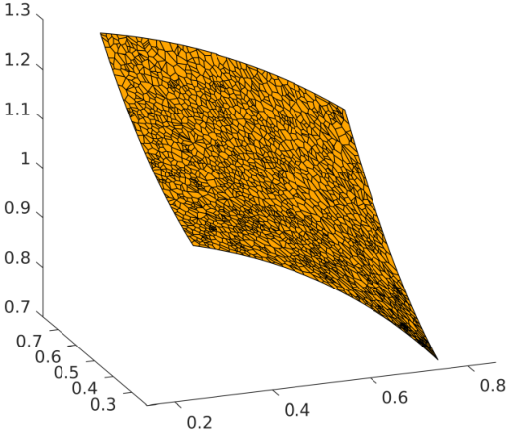
Here we consider a test problem originally proposed by Concus [14] that provided the following analytic solution to the minimal surface problem on the square Ω=(0.25,0.75)×(0.25,0.75)\Omega=(0.25,0.75)\times(0.25,0.75):

u⁡(x,y)=cosh2⁡(y)−x2.u(x,y)=\sqrt{\cosh^{2}(y)-x^{2}}.

Note that u∈H2​(Ω)∩W1,∞​(Ω)u\in H^{2}(\Omega)\cap W^{1,\infty}(\Omega). An example of computed solution on a coarse mesh is shown in Figure 2. Experiments are performed on uniform (Table 1) and random Voronoi meshes (Table 2). The assumption C⁡(uh)≲1C(u_{h})\lesssim 1 is verified and the rate of convergence in the H1H^{1}-norm is in agreement with Theorem 3.1. Moreover, the reported rate of convergence in the L2L^{2}-norm seems to be 22.

Refer to caption
(a)
Refer to caption
(b)
Figure 2: Example 4.1: example of the computational mesh (left) and corresponding computed solution (right).
Table 1: Example 4.1: computed errors and estimated convergence rates (uniform Voronoi meshes).
Mesh hh NN It eH1e_{H^{1}} ecr eL2e_{L^{2}} ecr C1C_{1} C2C_{2}
u-concus1 1.820 473⋅10−021.820\,473\text{\cdot}{10}^{-02} 40824082 1717 7.315 457⋅10−037.315\,457\text{\cdot}{10}^{-03} - 1.228 661⋅10−051.228\,661\text{\cdot}{10}^{-05} - 0.133 731 20.133\,731\,2 0.155 544 10.155\,544\,1
u-concus2 1.233 497⋅10−021.233\,497\text{\cdot}{10}^{-02} 81658165 1717 5.138 253⋅10−035.138\,253\text{\cdot}{10}^{-03} 1.019 1601.019\,160 6.175 387⋅10−066.175\,387\text{\cdot}{10}^{-06} 1.984 6191.984\,619 0.138 960 70.138\,960\,7 0.154 884 50.154\,884\,5
u-concus3 8.472 495⋅10−038.472\,495\text{\cdot}{10}^{-03} 16 32316\,323 1717 3.640 650⋅10−033.640\,650\text{\cdot}{10}^{-03} 0.994 7790.994\,779 3.206 931⋅10−063.206\,931\text{\cdot}{10}^{-06} 1.891 8431.891\,843 0.145 714 90.145\,714\,9 0.157 730 40.157\,730\,4
u-concus4 6.358 370⋅10−036.358\,370\text{\cdot}{10}^{-03} 32 65732\,657 1717 2.564 317⋅10−032.564\,317\text{\cdot}{10}^{-03} 1.010 7511.010\,751 1.521 949⋅10−061.521\,949\text{\cdot}{10}^{-06} 2.149 5022.149\,502 0.136 547 20.136\,547\,2 0.156 897 70.156\,897\,7
u-concus5 4.512 142⋅10−034.512\,142\text{\cdot}{10}^{-03} 65 29365\,293 1717 1.817 913⋅10−031.817\,913\text{\cdot}{10}^{-03} 0.993 0430.993\,043 7.959 064⋅10−077.959\,064\text{\cdot}{10}^{-07} 1.871 3671.871\,367 0.137 176 80.137\,176\,8 0.158 160 00.158\,160\,0
u-concus6 3.002 593⋅10−033.002\,593\text{\cdot}{10}^{-03} 130 567130\,567 1717 1.283 903⋅10−031.283\,903\text{\cdot}{10}^{-03} 1.003 7061.003\,706 4.037 045⋅10−074.037\,045\text{\cdot}{10}^{-07} 1.959 0101.959\,010 0.145 767 50.145\,767\,5 0.158 151 70.158\,151\,7
u-concus7 2.235 510⋅10−032.235\,510\text{\cdot}{10}^{-03} 261 206261\,206 1717 9.077 853⋅10−049.077\,853\text{\cdot}{10}^{-04} 0.999 8280.999\,828 1.979 326⋅10−071.979\,326\text{\cdot}{10}^{-07} 2.055 7622.055\,762 0.138 457 30.138\,457\,3 0.158 191 80.158\,191\,8
u-concus8 1.522 826⋅10−031.522\,826\text{\cdot}{10}^{-03} 522 279522\,279 1717 6.420 748⋅10−046.420\,748\text{\cdot}{10}^{-04} 0.999 5870.999\,587 9.936 792⋅10−089.936\,792\text{\cdot}{10}^{-08} 1.989 0451.989\,045 0.144 056 20.144\,056\,2 0.158 538 10.158\,538\,1
Table 2: Example 4.1: computed errors and estimated convergence rates (random Voronoi meshes).
Mesh hh NN It eH1e_{H^{1}} ecr eL2e_{L^{2}} ecr C1C_{1} C2C_{2}
concus1 3.406 596⋅10−023.406\,596\text{\cdot}{10}^{-02} 37163716 1717 9.316 064⋅10−039.316\,064\text{\cdot}{10}^{-03} - 2.736 716⋅10−052.736\,716\text{\cdot}{10}^{-05} - 0.091 030 100.091\,030\,10 0.189 035 60.189\,035\,6
concus2 2.526 368⋅10−022.526\,368\text{\cdot}{10}^{-02} 74507450 1717 6.407 736⋅10−036.407\,736\text{\cdot}{10}^{-03} 1.076 0571.076\,057 1.114 473⋅10−051.114\,473\text{\cdot}{10}^{-05} 2.583 1542.583\,154 0.083 715 360.083\,715\,36 0.182 549 10.182\,549\,1
concus3 1.717 608⋅10−021.717\,608\text{\cdot}{10}^{-02} 14 69314\,693 1717 4.582 240⋅10−034.582\,240\text{\cdot}{10}^{-03} 0.987 4530.987\,453 5.944 094⋅10−065.944\,094\text{\cdot}{10}^{-06} 1.851 0261.851\,026 0.089 057 510.089\,057\,51 0.185 417 10.185\,417\,1
concus4 1.293 438⋅10−021.293\,438\text{\cdot}{10}^{-02} 29 48729\,487 1717 3.223 429⋅10−033.223\,429\text{\cdot}{10}^{-03} 1.009 9151.009\,915 3.044 994⋅10−063.044\,994\text{\cdot}{10}^{-06} 1.920 5291.920\,529 0.083 530 300.083\,530\,30 0.185 526 10.185\,526\,1
concus5 9.161 274⋅10−039.161\,274\text{\cdot}{10}^{-03} 59 01159\,011 1717 2.263 267⋅10−032.263\,267\text{\cdot}{10}^{-03} 1.019 4561.019\,456 1.581 828⋅10−061.581\,828\text{\cdot}{10}^{-06} 1.887 9841.887\,984 0.083 040 980.083\,040\,98 0.184 805 50.184\,805\,5
concus6 7.240 372⋅10−037.240\,372\text{\cdot}{10}^{-03} 118 053118\,053 1717 1.601 315⋅10−031.601\,315\text{\cdot}{10}^{-03} 0.997 9210.997\,921 7.453 749⋅10−077.453\,749\text{\cdot}{10}^{-07} 2.170 2872.170\,287 0.074 488 090.074\,488\,09 0.185 304 60.185\,304\,6
concus7 4.918 414⋅10−034.918\,414\text{\cdot}{10}^{-03} 235 898235\,898 1717 1.134 128⋅10−031.134\,128\text{\cdot}{10}^{-03} 0.996 6150.996\,615 3.709 904⋅10−073.709\,904\text{\cdot}{10}^{-07} 2.015 7322.015\,732 0.077 542 010.077\,542\,01 0.185 235 50.185\,235\,5
concus8 3.568 262⋅10−033.568\,262\text{\cdot}{10}^{-03} 472 263472\,263 1717 8.009 051⋅10−048.009\,051\text{\cdot}{10}^{-04} 1.002 3301.002\,330 1.840 569⋅10−071.840\,569\text{\cdot}{10}^{-07} 2.019 5772.019\,577 0.075 568 600.075\,568\,60 0.185 306 20.185\,306\,2

4.2 Test 2

Here we consider another test problem for which an analytic solution is known [18]. Let us consider the following convex domain

Ω={𝐱=(x,y)∈ℝ2|∥𝐱∥2<4∩x>1}.\Omega=\Set{\mathbf{x}=(x,y)\in\mathbb{R}^{2}}{\lVert\mathbf{x}\rVert_{2}<4\cap x>1}.

An explicit example of minimal surface on Ω\Omega is given by

u⁡(x,y)=a​log⁡(b+b2−a2r+r2−a2),u(x,y)=a\log\left(\frac{b+\sqrt{b^{2}-a^{2}}}{r+\sqrt{r^{2}-a^{2}}}\right),

where we take a=0.75,b=4a=0.75,b=4 and r=x2+y2r=\sqrt{x^{2}+y^{2}}. Note that u∈H2​(Ω)∩W1,∞​(Ω)u\in H^{2}(\Omega)\cap W^{1,\infty}(\Omega). This minimal surface is also known as catenoid. A typical solution on a coarse mesh is shown in Figure 3. Experiments are performed on uniform Voronoi meshes (Table 3) and random Voronoi meshes (Table 4). Again, C⁡(uh)≲1C(u_{h})\lesssim 1 and the rate of convergence in the H1H^{1}-norm is in agreement with Theorem 3.1, whereas the computed rate of convergence in the L2L^{2}-norm seems to be 22.

Refer to caption
(a)
Refer to caption
(b)
Figure 3: Example 4.2: example of the computational mesh (left) and corresponding computed solution (right).
Table 3: Example 4.2: computed errors and estimated convergence rates (uniform Voronoi meshes).
Mesh hh NN It eH1e_{H^{1}} ecr eL2e_{L^{2}} ecr C1C_{1} C2C_{2}
u-sector1 1.408 847⋅10−011.408\,847\text{\cdot}{10}^{-01} 40804080 2020 2.571 832⋅10−022.571\,832\text{\cdot}{10}^{-02} - 3.745 642⋅10−043.745\,642\text{\cdot}{10}^{-04} - 0.198 1310.198\,131 1.782 9791.782\,979
u-sector2 1.031 659⋅10−011.031\,659\text{\cdot}{10}^{-01} 81588158 2121 1.748 529⋅10−021.748\,529\text{\cdot}{10}^{-02} 1.113 7041.113\,704 1.720 191⋅10−041.720\,191\text{\cdot}{10}^{-04} 2.246 0832.246\,083 0.186 4100.186\,410 1.736 9901.736\,990
u-sector3 6.978 080⋅10−026.978\,080\text{\cdot}{10}^{-02} 16 30916\,309 2121 1.262 748⋅10−021.262\,748\text{\cdot}{10}^{-02} 0.939 7310.939\,731 8.938 975⋅10−058.938\,975\text{\cdot}{10}^{-05} 1.889 9451.889\,945 0.198 4210.198\,421 1.768 2271.768\,227
u-sector4 5.177 668⋅10−025.177\,668\text{\cdot}{10}^{-02} 32 64032\,640 2222 8.940 494⋅10−038.940\,494\text{\cdot}{10}^{-03} 0.995 3120.995\,312 4.514 633⋅10−054.514\,633\text{\cdot}{10}^{-05} 1.969 0861.969\,086 0.187 9090.187\,909 1.757 7461.757\,746
u-sector5 3.587 076⋅10−023.587\,076\text{\cdot}{10}^{-02} 65 27165\,271 2222 6.378 085⋅10−036.378\,085\text{\cdot}{10}^{-03} 0.974 6560.974\,656 2.291 350⋅10−052.291\,350\text{\cdot}{10}^{-05} 1.957 2111.957\,211 0.194 1610.194\,161 1.779 3581.779\,358
u-sector6 2.557 910⋅10−022.557\,910\text{\cdot}{10}^{-02} 130 572130\,572 2323 4.431 724⋅10−034.431\,724\text{\cdot}{10}^{-03} 1.050 1631.050\,163 1.115 385⋅10−051.115\,385\text{\cdot}{10}^{-05} 2.076 6242.076\,624 0.188 3800.188\,380 1.741 1811.741\,181
u-sector7 1.807 119⋅10−021.807\,119\text{\cdot}{10}^{-02} 261 077261\,077 2323 3.140 899⋅10−033.140\,899\text{\cdot}{10}^{-03} 0.993 7490.993\,749 5.583 417⋅10−065.583\,417\text{\cdot}{10}^{-06} 1.997 3821.997\,382 0.190 1670.190\,167 1.755 9281.755\,928
u-sector8 1.296 064⋅10−021.296\,064\text{\cdot}{10}^{-02} 522 210522\,210 2323 2.216 130⋅10−032.216\,130\text{\cdot}{10}^{-03} 1.006 1141.006\,114 2.763 452⋅10−062.763\,452\text{\cdot}{10}^{-06} 2.029 0402.029\,040 0.187 9930.187\,993 1.760 7221.760\,722
Table 4: Example 4.2: computed errors and estimated convergence rates (random Voronoi meshes).
Mesh hh NN It eH1e_{H^{1}} ecr eL2e_{L^{2}} ecr C1C_{1} C2C_{2}
sector1 2.783 233⋅10−012.783\,233\text{\cdot}{10}^{-01} 41984198 1919 3.037 020⋅10−023.037\,020\text{\cdot}{10}^{-02} - 6.536 296⋅10−046.536\,296\text{\cdot}{10}^{-04} - 0.121 0570.121\,057 2.183 0392.183\,039
sector2 2.262 086⋅10−012.262\,086\text{\cdot}{10}^{-01} 83308330 1919 2.303 112⋅10−022.303\,112\text{\cdot}{10}^{-02} 0.807 3360.807\,336 3.991 139⋅10−043.991\,139\text{\cdot}{10}^{-04} 1.439 7381.439\,738 0.109 9300.109\,930 2.269 5952.269\,595
sector3 1.475 084⋅10−011.475\,084\text{\cdot}{10}^{-01} 16 58816\,588 2121 1.536 174⋅10−021.536\,174\text{\cdot}{10}^{-02} 1.175 8341.175\,834 1.606 314⋅10−041.606\,314\text{\cdot}{10}^{-04} 2.642 6062.642\,606 0.114 7470.114\,747 2.179 9862.179\,986
sector4 1.074 039⋅10−011.074\,039\text{\cdot}{10}^{-01} 33 08033\,080 2222 1.106 745⋅10−021.106\,745\text{\cdot}{10}^{-02} 0.950 0090.950\,009 8.749 437⋅10−058.749\,437\text{\cdot}{10}^{-05} 1.760 3431.760\,343 0.113 6710.113\,671 2.220 5122.220\,512
sector5 7.993 085⋅10−027.993\,085\text{\cdot}{10}^{-02} 65 97365\,973 2222 7.805 126⋅10−037.805\,126\text{\cdot}{10}^{-03} 1.011 7901.011\,790 4.463 371⋅10−054.463\,371\text{\cdot}{10}^{-05} 1.950 0761.950\,076 0.108 6300.108\,630 2.230 2212.230\,221
sector6 5.475 817⋅10−025.475\,817\text{\cdot}{10}^{-02} 131 673131\,673 2323 5.477 103⋅10−035.477\,103\text{\cdot}{10}^{-03} 1.025 0811.025\,081 2.080 637⋅10−052.080\,637\text{\cdot}{10}^{-05} 2.208 8162.208\,816 0.111 2980.111\,298 2.211 4942.211\,494
sector7 4.037 713⋅10−024.037\,713\text{\cdot}{10}^{-02} 262 975262\,975 2323 3.897 524⋅10−033.897\,524\text{\cdot}{10}^{-03} 0.983 7110.983\,711 1.057 072⋅10−051.057\,072\text{\cdot}{10}^{-05} 1.957 8861.957\,886 0.108 4410.108\,441 2.245 3692.245\,369
sector8 2.853 023⋅10−022.853\,023\text{\cdot}{10}^{-02} 525 468525\,468 2323 2.724 878⋅10−032.724\,878\text{\cdot}{10}^{-03} 1.034 1001.034\,100 5.122 127⋅10−065.122\,127\text{\cdot}{10}^{-06} 2.093 2862.093\,286 0.107 7320.107\,732 2.228 0422.228\,042

4.3 Test 3

Here we consider the so called Scherk’s fifth surface [19] which is another minimal surface that can be expressed on Ω=(−0.8,0.8)×(−0.8,0.8)\Omega=(-0.8,0.8)\times(-0.8,0.8) as follows

u⁡(x,y)=sin−1⁡(sinh⁡x​sinh⁡y).u(x,y)=\sin^{-1}(\sinh x\sinh y).

A typical solution on a coarse mesh is shown in Figure 4. Experiments are performed on uniform Voronoi meshes (Table 5) and random Voronoi meshes (Table 6). The assumption C⁡(uh)≲1C(u_{h})\lesssim 1 is satisfied, and, as predicted by our theoretical analysis, we observe a linear convergence in the H1H^{1} norm. Moreover, second order convergence in the L2L^{2} norm is also observed.

Refer to caption
(a)
Refer to caption
(b)
Figure 4: Example 4.3: example of the computational mesh (left) and corresponding computed solution (right).
Table 5: Example 4.3: computed errors and estimated convergence rates (uniform Voronoi meshes).
Mesh hh NN It eH1e_{H^{1}} ecr eL2e_{L^{2}} ecr C1C_{1} C2C_{2}
u-scherk1 5.845 703⋅10−025.845\,703\text{\cdot}{10}^{-02} 40794079 2525 2.830 468⋅10−022.830\,468\text{\cdot}{10}^{-02} - 7.509 648⋅10−047.509\,648\text{\cdot}{10}^{-04} - 0.550 2090.550\,209 2.054 1932.054\,193
u-scherk2 3.876 636⋅10−023.876\,636\text{\cdot}{10}^{-02} 81588158 2727 1.972 075⋅10−021.972\,075\text{\cdot}{10}^{-02} 1.042 6521.042\,652 3.571 190⋅10−043.571\,190\text{\cdot}{10}^{-04} 2.144 6812.144\,681 0.563 2180.563\,218 1.972 0771.972\,077
u-scherk3 2.792 674⋅10−022.792\,674\text{\cdot}{10}^{-02} 16 32316\,323 2929 1.396 771⋅10−021.396\,771\text{\cdot}{10}^{-02} 0.994 6220.994\,622 1.802 687⋅10−041.802\,687\text{\cdot}{10}^{-04} 1.971 2921.971\,292 0.547 9370.547\,937 1.955 0201.955\,020
u-scherk4 1.959 732⋅10−021.959\,732\text{\cdot}{10}^{-02} 32 66432\,664 3131 9.785 263⋅10−039.785\,263\text{\cdot}{10}^{-03} 1.026 0111.026\,011 8.673 115⋅10−058.673\,115\text{\cdot}{10}^{-05} 2.109 3762.109\,376 0.541 9210.541\,921 1.919 4081.919\,408
u-scherk5 1.382 014⋅10−021.382\,014\text{\cdot}{10}^{-02} 65 27565\,275 2929 6.986 006⋅10−036.986\,006\text{\cdot}{10}^{-03} 0.973 4250.973\,425 4.502 900⋅10−054.502\,900\text{\cdot}{10}^{-05} 1.893 6091.893\,609 0.540 5280.540\,528 1.908 5531.908\,553
u-scherk6 1.008 418⋅10−021.008\,418\text{\cdot}{10}^{-02} 130 555130\,555 3030 4.922 164⋅10−034.922\,164\text{\cdot}{10}^{-03} 1.010 2951.010\,295 2.266 426⋅10−052.266\,426\text{\cdot}{10}^{-05} 1.980 7611.980\,761 0.518 6310.518\,631 1.889 7131.889\,713
u-scherk7 7.062 998⋅10−037.062\,998\text{\cdot}{10}^{-03} 261 164261\,164 3131 3.484 116⋅10−033.484\,116\text{\cdot}{10}^{-03} 0.996 7030.996\,703 1.123 266⋅10−051.123\,266\text{\cdot}{10}^{-05} 2.024 8352.024\,835 0.522 6500.522\,650 1.886 5001.886\,500
u-scherk8 5.043 997⋅10−035.043\,997\text{\cdot}{10}^{-03} 522 210522\,210 3030 2.472 460⋅10−032.472\,460\text{\cdot}{10}^{-03} 0.990 0130.990\,013 5.611 956⋅10−065.611\,956\text{\cdot}{10}^{-06} 2.002 9012.002\,901 0.517 1340.517\,134 1.884 9521.884\,952
Table 6: Example 4.3: computed errors and estimated convergence rates (random Voronoi meshes).
Mesh hh NN It eH1e_{H^{1}} ecr eL2e_{L^{2}} ecr C1C_{1} C2C_{2}
scherk1 1.182 205⋅10−011.182\,205\text{\cdot}{10}^{-01} 40984098 2929 3.544 840⋅10−023.544\,840\text{\cdot}{10}^{-02} - 1.450 268⋅10−031.450\,268\text{\cdot}{10}^{-03} - 0.312 3190.312\,319 2.363 6192.363\,619
scherk2 7.672 309⋅10−027.672\,309\text{\cdot}{10}^{-02} 81978197 3131 2.444 451⋅10−022.444\,451\text{\cdot}{10}^{-02} 1.072 2321.072\,232 6.571 025⋅10−046.571\,025\text{\cdot}{10}^{-04} 2.283 8572.283\,857 0.333 4820.333\,482 2.316 4652.316\,465
scherk3 5.475 856⋅10−025.475\,856\text{\cdot}{10}^{-02} 16 39116\,391 3434 1.761 149⋅10−021.761\,149\text{\cdot}{10}^{-02} 0.946 2360.946\,236 3.761 298⋅10−043.761\,298\text{\cdot}{10}^{-04} 1.610 2011.610\,201 0.328 4000.328\,400 2.302 2822.302\,282
scherk4 4.149 791⋅10−024.149\,791\text{\cdot}{10}^{-02} 32 77832\,778 3434 1.254 106⋅10−021.254\,106\text{\cdot}{10}^{-02} 0.979 8870.979\,887 1.727 792⋅10−041.727\,792\text{\cdot}{10}^{-04} 2.244 9982.244\,998 0.310 4220.310\,422 2.332 2192.332\,219
scherk5 2.848 743⋅10−022.848\,743\text{\cdot}{10}^{-02} 65 55165\,551 3333 8.769 878⋅10−038.769\,878\text{\cdot}{10}^{-03} 1.032 1761.032\,176 8.586 859⋅10−058.586\,859\text{\cdot}{10}^{-05} 2.017 6762.017\,676 0.316 2250.316\,225 2.306 4252.306\,425
scherk6 2.126 006⋅10−022.126\,006\text{\cdot}{10}^{-02} 131 087131\,087 3636 6.221 969⋅10−036.221\,969\text{\cdot}{10}^{-03} 0.990 5350.990\,535 4.452 327⋅10−054.452\,327\text{\cdot}{10}^{-05} 1.895 4551.895\,455 0.300 5260.300\,526 2.313 2712.313\,271
scherk7 1.751 864⋅10−021.751\,864\text{\cdot}{10}^{-02} 262 167262\,167 3535 4.353 764⋅10−034.353\,764\text{\cdot}{10}^{-03} 1.030 2561.030\,256 2.098 014⋅10−052.098\,014\text{\cdot}{10}^{-05} 2.171 1542.171\,154 0.255 5590.255\,559 2.292 3452.292\,345
scherk8 1.078 938⋅10−021.078\,938\text{\cdot}{10}^{-02} 524 326524\,326 3232 3.101 653⋅10−033.101\,653\text{\cdot}{10}^{-03} 0.978 4740.978\,474 1.076 297⋅10−051.076\,297\text{\cdot}{10}^{-05} 1.925 9381.925\,938 0.293 8960.293\,896 2.296 0972.296\,097

4.4 Test 4

The minimal surface problem (4) is solved on Ω=(0,1)2\Omega=(0,1)^{2} with the following boundary conditions

{φ=0 on ​y=0​ and ​x=0,φ=x on ​y=1,φ=y on ​x=1.\begin{cases}\varphi=0&\text{ on }y=0\text{ and }x=0,\\ \varphi=x&\text{ on }y=1,\\ \varphi=y&\text{ on }x=1.\end{cases}

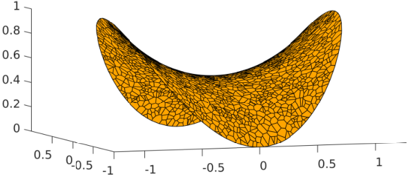
A typical solution on a coarse mesh is shown in Figure 5. We recall that by properly rotating and translating this minimal surface, it is possible to obtain the so-called Schwarz D surface (see Figure 6). Results on uniform and random Voronoi meshes are shown in Tables 7 and 8, respectively. The reference FEM solution is computed on a Delaunay triangular mesh with 77675837767583 nodes and 1552462715524627 triangles. Also in this case we observe C⁡(uh)≲1C(u_{h})\lesssim 1, a linear convergence in the H1H^{1} norm, and a quadratic convergence in the L2L^{2} norm.

Refer to caption
(a)
Refer to caption
(b)
Figure 5: Example 4.4: example of the computational mesh (left) and corresponding computed solution (right).
Refer to caption
Figure 6: Example 4.4: representation of the Schwarz D surface obtained by rotating and translating the patch shown in Figure 5.
Table 7: Example 4.4: computed errors and estimated convergence rates (uniform Voronoi meshes).
Mesh hh NN It eH1e_{H^{1}} ecr eL2e_{L^{2}} ecr C1C_{1} C2C_{2}
u-square1 3.400 609⋅10−023.400\,609\text{\cdot}{10}^{-02} 40774077 2222 1.138 459⋅10−021.138\,459\text{\cdot}{10}^{-02} - 1.118 740⋅10−041.118\,740\text{\cdot}{10}^{-04} - 0.229 8880.229\,888 0.499 1630.499\,163
u-square2 2.698 981⋅10−022.698\,981\text{\cdot}{10}^{-02} 81558155 2222 8.004 869⋅10−038.004\,869\text{\cdot}{10}^{-03} 1.016 0861.016\,086 5.503 866⋅10−055.503\,866\text{\cdot}{10}^{-05} 2.046 3542.046\,354 0.203 0070.203\,007 0.494 7910.494\,791
u-square3 1.740 063⋅10−021.740\,063\text{\cdot}{10}^{-02} 16 32516\,325 2222 5.697 379⋅10−035.697\,379\text{\cdot}{10}^{-03} 0.979 8590.979\,859 2.781 825⋅10−052.781\,825\text{\cdot}{10}^{-05} 1.966 2201.966\,220 0.222 4030.222\,403 0.494 4620.494\,462
u-square4 1.211 312⋅10−021.211\,312\text{\cdot}{10}^{-02} 32 63632\,636 2222 4.022 932⋅10−034.022\,932\text{\cdot}{10}^{-03} 1.004 7241.004\,724 1.387 913⋅10−051.387\,913\text{\cdot}{10}^{-05} 2.007 4722.007\,472 0.225 8230.225\,823 0.494 1650.494\,165
u-square5 8.695 573⋅10−038.695\,573\text{\cdot}{10}^{-03} 65 29765\,297 2222 2.848 237⋅10−032.848\,237\text{\cdot}{10}^{-03} 0.995 8060.995\,806 6.894 715⋅10−066.894\,715\text{\cdot}{10}^{-06} 2.017 5942.017\,594 0.221 1700.221\,170 0.491 4420.491\,442
u-square6 6.110 583⋅10−036.110\,583\text{\cdot}{10}^{-03} 130 532130\,532 2222 2.021 494⋅10−032.021\,494\text{\cdot}{10}^{-03} 0.989 9730.989\,973 3.443 489⋅10−063.443\,489\text{\cdot}{10}^{-06} 2.004 6142.004\,614 0.221 4520.221\,452 0.488 9000.488\,900
u-square7 4.472 890⋅10−034.472\,890\text{\cdot}{10}^{-03} 261 135261\,135 2222 1.437 691⋅10−031.437\,691\text{\cdot}{10}^{-03} 0.982 9500.982\,950 1.721 962⋅10−061.721\,962\text{\cdot}{10}^{-06} 1.998 8511.998\,851 0.213 7860.213\,786 0.488 6520.488\,652
u-square8 3.113 299⋅10−033.113\,299\text{\cdot}{10}^{-03} 522 236522\,236 2222 1.028 641⋅10−031.028\,641\text{\cdot}{10}^{-03} 0.966 1200.966\,120 8.599 788⋅10−078.599\,788\text{\cdot}{10}^{-07} 2.003 5492.003\,549 0.217 1320.217\,132 0.488 5140.488\,514
Table 8: Example 4.4: computed errors and estimated convergence rates (random Voronoi meshes).
Mesh hh NN It eH1e_{H^{1}} ecr eL2e_{L^{2}} ecr C1C_{1} C2C_{2}
square1 6.384 666⋅10−026.384\,666\text{\cdot}{10}^{-02} 50065006 2222 1.282 674⋅10−021.282\,674\text{\cdot}{10}^{-02} - 1.712 198⋅10−041.712\,198\text{\cdot}{10}^{-04} - 0.135 7630.135\,763 0.613 2910.613\,291
square2 4.344 562⋅10−024.344\,562\text{\cdot}{10}^{-02} 10 00810\,008 2222 9.094 385⋅10−039.094\,385\text{\cdot}{10}^{-03} 0.992 7850.992\,785 8.512 310⋅10−058.512\,310\text{\cdot}{10}^{-05} 2.017 6182.017\,618 0.142 3510.142\,351 0.618 7010.618\,701
square3 3.470 002⋅10−023.470\,002\text{\cdot}{10}^{-02} 20 00720\,007 2222 6.384 179⋅10−036.384\,179\text{\cdot}{10}^{-03} 1.021 6131.021\,613 4.187 674⋅10−054.187\,674\text{\cdot}{10}^{-05} 2.048 1322.048\,132 0.125 8490.125\,849 0.617 6910.617\,691
square4 2.405 393⋅10−022.405\,393\text{\cdot}{10}^{-02} 40 01140\,011 2222 4.511 768⋅10−034.511\,768\text{\cdot}{10}^{-03} 1.001 7241.001\,724 2.082 425⋅10−052.082\,425\text{\cdot}{10}^{-05} 2.015 9882.015\,988 0.127 5080.127\,508 0.613 4960.613\,496
square5 1.726 980⋅10−021.726\,980\text{\cdot}{10}^{-02} 80 00780\,007 2222 3.210 831⋅10−033.210\,831\text{\cdot}{10}^{-03} 0.981 7580.981\,758 1.058 687⋅10−051.058\,687\text{\cdot}{10}^{-05} 1.952 5041.952\,504 0.126 6510.126\,651 0.618 6700.618\,670
square6 1.140 086⋅10−021.140\,086\text{\cdot}{10}^{-02} 160 028160\,028 2222 2.268 962⋅10−032.268\,962\text{\cdot}{10}^{-03} 1.001 7021.001\,702 5.246 371⋅10−065.246\,371\text{\cdot}{10}^{-06} 2.025 5142.025\,514 0.135 1020.135\,102 0.616 1670.616\,167
square7 8.860 795⋅10−038.860\,795\text{\cdot}{10}^{-03} 320 020320\,020 2222 1.613 746⋅10−031.613\,746\text{\cdot}{10}^{-03} 0.983 3980.983\,398 2.630 185⋅10−062.630\,185\text{\cdot}{10}^{-06} 1.992 6351.992\,635 0.123 1530.123\,153 0.617 3150.617\,315
square8 6.248 831⋅10−036.248\,831\text{\cdot}{10}^{-03} 640 035640\,035 2222 1.149 771⋅10−031.149\,771\text{\cdot}{10}^{-03} 0.978 1440.978\,144 1.308 687⋅10−061.308\,687\text{\cdot}{10}^{-06} 2.014 1102.014\,110 0.123 2950.123\,295 0.616 3750.616\,375

4.5 Test 5

Here we consider a minimal surface problem on the unit disk, where the boundary condition is φ⁡(x,y)=x2\varphi(x,y)=x^{2}. A typical solution on a coarse mesh is shown in Figure 7. Results on uniform and random Voronoi meshes are shown in Tables 9 and 10, respectively. Again, C⁡(uh)≲1C(u_{h})\lesssim 1 and we observe a linear convergence in the H1H^{1} norm. Moreover, second order convergence in the L2L^{2} norm is also observed.

Refer to caption
(a)
Refer to caption
(b)
Figure 7: Example 4.5: example of the computational mesh (left) and corresponding computed solution (right).
Table 9: Example 4.5: computed errors and estimated convergence rates (uniform Voronoi meshes).
Mesh hh NN It eH1e_{H^{1}} ecr eL2e_{L^{2}} ecr C1C_{1} C2C_{2}
u-circ1 6.167 744⋅10−026.167\,744\text{\cdot}{10}^{-02} 40744074 2222 2.491 744⋅10−022.491\,744\text{\cdot}{10}^{-02} - 2.175 920⋅10−042.175\,920\text{\cdot}{10}^{-04} - 0.416 6370.416\,637 1.640 1931.640\,193
u-circ2 4.246 809⋅10−024.246\,809\text{\cdot}{10}^{-02} 81668166 2222 1.759 650⋅10−021.759\,650\text{\cdot}{10}^{-02} 1.000 5481.000\,548 1.086 885⋅10−041.086\,885\text{\cdot}{10}^{-04} 1.996 4961.996\,496 0.427 7840.427\,784 1.641 6951.641\,695
u-circ3 3.054 830⋅10−023.054\,830\text{\cdot}{10}^{-02} 16 30316\,303 2222 1.243 710⋅10−021.243\,710\text{\cdot}{10}^{-02} 1.003 8501.003\,850 5.396 769⋅10−055.396\,769\text{\cdot}{10}^{-05} 2.025 2562.025\,256 0.422 1850.422\,185 1.646 7331.646\,733
u-circ4 2.163 149⋅10−022.163\,149\text{\cdot}{10}^{-02} 32 61932\,619 2222 8.797 412⋅10−038.797\,412\text{\cdot}{10}^{-03} 0.998 4250.998\,425 2.688 975⋅10−052.688\,975\text{\cdot}{10}^{-05} 2.008 9242.008\,924 0.416 1590.416\,159 1.625 8521.625\,852
u-circ5 1.506 714⋅10−021.506\,714\text{\cdot}{10}^{-02} 65 27565\,275 2323 6.232 316⋅10−036.232\,316\text{\cdot}{10}^{-03} 0.993 8090.993\,809 1.346 466⋅10−051.346\,466\text{\cdot}{10}^{-05} 1.994 1261.994\,126 0.425 0500.425\,050 1.636 2291.636\,229
u-circ6 1.064 505⋅10−021.064\,505\text{\cdot}{10}^{-02} 130 546130\,546 2323 4.427 231⋅10−034.427\,231\text{\cdot}{10}^{-03} 0.986 7710.986\,771 6.718 177⋅10−066.718\,177\text{\cdot}{10}^{-06} 2.006 1612.006\,161 0.425 5040.425\,504 1.636 5641.636\,564
u-circ7 7.731 530⋅10−037.731\,530\text{\cdot}{10}^{-03} 261 069261\,069 2323 3.158 871⋅10−033.158\,871\text{\cdot}{10}^{-03} 0.974 1150.974\,115 3.354 122⋅10−063.354\,122\text{\cdot}{10}^{-06} 2.004 5242.004\,524 0.414 4190.414\,419 1.637 1271.637\,127
u-circ8 5.459 296⋅10−035.459\,296\text{\cdot}{10}^{-03} 522 188522\,188 2323 2.274 585⋅10−032.274\,585\text{\cdot}{10}^{-03} 0.947 4800.947\,480 1.675 214⋅10−061.675\,214\text{\cdot}{10}^{-06} 2.002 9032.002\,903 0.414 5890.414\,589 1.635 5651.635\,565
Table 10: Example 4.5: computed errors and estimated convergence rates (random Voronoi meshes).
Mesh hh NN It eH1e_{H^{1}} ecr eL2e_{L^{2}} ecr C1C_{1} C2C_{2}
circ1 1.207 272⋅10−011.207\,272\text{\cdot}{10}^{-01} 42384238 2121 3.111 517⋅10−023.111\,517\text{\cdot}{10}^{-02} - 4.282 237⋅10−044.282\,237\text{\cdot}{10}^{-04} - 0.271 2030.271\,203 2.131 4722.131\,472
circ2 8.719 227⋅10−028.719\,227\text{\cdot}{10}^{-02} 83988398 2222 2.187 564⋅10−022.187\,564\text{\cdot}{10}^{-02} 1.030 3281.030\,328 2.050 550⋅10−042.050\,550\text{\cdot}{10}^{-04} 2.153 4302.153\,430 0.264 4880.264\,488 2.113 3512.113\,351
circ3 6.233 188⋅10−026.233\,188\text{\cdot}{10}^{-02} 16 66216\,662 2222 1.545 690⋅10−021.545\,690\text{\cdot}{10}^{-02} 1.013 8651.013\,865 1.021 701⋅10−041.021\,701\text{\cdot}{10}^{-04} 2.033 5752.033\,575 0.260 6360.260\,636 2.097 0442.097\,044
circ4 4.554 244⋅10−024.554\,244\text{\cdot}{10}^{-02} 33 17533\,175 2222 1.094 648⋅10−021.094\,648\text{\cdot}{10}^{-02} 1.002 0481.002\,048 5.069 568⋅10−055.069\,568\text{\cdot}{10}^{-05} 2.035 2362.035\,236 0.253 4730.253\,473 2.102 5822.102\,582
circ5 3.382 851⋅10−023.382\,851\text{\cdot}{10}^{-02} 66 09666\,096 2323 7.744 545⋅10−037.744\,545\text{\cdot}{10}^{-03} 1.003 9841.003\,984 2.544 399⋅10−052.544\,399\text{\cdot}{10}^{-05} 2.000 1442.000\,144 0.239 3610.239\,361 2.081 7282.081\,728
circ6 2.421 469⋅10−022.421\,469\text{\cdot}{10}^{-02} 131 883131\,883 2323 5.479 975⋅10−035.479\,975\text{\cdot}{10}^{-03} 1.001 4031.001\,403 1.264 160⋅10−051.264\,160\text{\cdot}{10}^{-05} 2.025 1282.025\,128 0.237 0220.237\,022 2.084 3102.084\,310
circ7 1.804 084⋅10−021.804\,084\text{\cdot}{10}^{-02} 263 268263\,268 2323 3.898 897⋅10−033.898\,897\text{\cdot}{10}^{-03} 0.984 8920.984\,892 6.310 083⋅10−066.310\,083\text{\cdot}{10}^{-06} 2.010 3782.010\,378 0.224 9700.224\,970 2.082 4812.082\,481
circ8 1.199 765⋅10−021.199\,765\text{\cdot}{10}^{-02} 525 901525\,901 2323 2.783 893⋅10−032.783\,893\text{\cdot}{10}^{-03} 0.973 6190.973\,619 3.121 175⋅10−063.121\,175\text{\cdot}{10}^{-06} 2.034 6812.034\,681 0.238 7400.238\,740 2.077 1792.077\,179

4.6 Test 6

In the last example, the minimal surface problem is again solved on Ω=(0,1)2\Omega=(0,1)^{2}. As Dirichlet boundary conditions, we require the solution to match proper reflections of the fourth iterate of a sequence of functions converging to the Cantor function (see Figure 8). Note that the exact solution does not satisfy the regularity assumptions of Theorem 3.1.

(a)
(b)
Figure 8: Example 4.6: fourth iterate of a sequence of function converging to the Cantor function on [0,1][0,1] (left) which is used as as boundary condition for Example 4.6 (right).

A typical solution on a coarse mesh is shown in Figure 9. Results on uniform and random Voronoi meshes are shown in Tables 11 and 12, respectively. The reference FEM solution is computed on a Delaunay triangular mesh with 77680417768041 nodes and 1552505115525051 triangles. Such mesh is constructed in order to have all the nodes where the Dirichlet data is just continuous as boundary nodes. Observe that the assumption C⁡(uh)≲1C(u_{h})\lesssim 1 does not hold in this case. This example shows that a lack of regularity in the boundary data may severely affect the convergence properties of the method.

Refer to caption
(a)
Refer to caption
(b)
Figure 9: Example 4.6: example of the computational mesh (left) and corresponding computed solution (right).
Table 11: Example 4.6: computed errors and estimated convergence rates (uniform Voronoi meshes).
Mesh hh NN It eH1e_{H^{1}} ecr eL2e_{L^{2}} ecr C1C_{1} C2C_{2}
u-square1 3.400 609⋅10−023.400\,609\text{\cdot}{10}^{-02} 40774077 3131 4.609 498⋅10−014.609\,498\text{\cdot}{10}^{-01} - 3.013 669⋅10−023.013\,669\text{\cdot}{10}^{-02} - 3.374 8113.374\,811 7.327 8507.327\,850
u-square2 2.698 981⋅10−022.698\,981\text{\cdot}{10}^{-02} 81558155 4545 4.194 200⋅10−014.194\,200\text{\cdot}{10}^{-01} 0.272 3800.272\,380 2.415 286⋅10−022.415\,286\text{\cdot}{10}^{-02} 0.638 5410.638\,541 3.983 6813.983\,681 9.709 4869.709\,486
u-square3 1.740 063⋅10−021.740\,063\text{\cdot}{10}^{-02} 16 32516\,325 4545 3.902 435⋅10−013.902\,435\text{\cdot}{10}^{-01} 0.207 7670.207\,767 2.114 981⋅10−022.114\,981\text{\cdot}{10}^{-02} 0.382 5910.382\,591 6.553 7326.553\,732 14.570 69814.570\,698
u-square4 1.211 312⋅10−021.211\,312\text{\cdot}{10}^{-02} 32 63632\,636 4646 2.826 745⋅10−012.826\,745\text{\cdot}{10}^{-01} 0.931 0420.931\,042 4.374 640⋅10−034.374\,640\text{\cdot}{10}^{-03} 4.549 6324.549\,632 7.861 1737.861\,173 17.202 51017.202\,510
u-square5 8.695 573⋅10−038.695\,573\text{\cdot}{10}^{-03} 65 29765\,297 5959 3.419 749⋅10−013.419\,749\text{\cdot}{10}^{-01} −0.549 193-0.549\,193 1.280 841⋅10−021.280\,841\text{\cdot}{10}^{-02} −3.097 998-3.097\,998 9.116 7059.116\,705 20.257 35520.257\,355
u-square6 6.110 583⋅10−036.110\,583\text{\cdot}{10}^{-03} 130 532130\,532 6767 3.683 411⋅10−013.683\,411\text{\cdot}{10}^{-01} −0.214 451-0.214\,451 1.364 939⋅10−021.364\,939\text{\cdot}{10}^{-02} −0.183 617-0.183\,617 10.450 64810.450\,648 23.071 95323.071\,953
u-square7 4.472 890⋅10−034.472\,890\text{\cdot}{10}^{-03} 261 135261\,135 8484 2.695 212⋅10−012.695\,212\text{\cdot}{10}^{-01} 0.900 9340.900\,934 6.281 133⋅10−036.281\,133\text{\cdot}{10}^{-03} 2.238 6022.238\,602 11.192 52311.192\,523 25.582 83925.582\,839
u-square8 3.113 299⋅10−033.113\,299\text{\cdot}{10}^{-03} 522 236522\,236 100100 3.079 599⋅10−013.079\,599\text{\cdot}{10}^{-01} −0.384 724-0.384\,724 7.085 787⋅10−037.085\,787\text{\cdot}{10}^{-03} −0.347 839-0.347\,839 12.481 80212.481\,802 28.082 22628.082\,226
Table 12: Example 4.6: computed errors and estimated convergence rates (random Voronoi meshes).
Mesh hh NN It eH1e_{H^{1}} ecr eL2e_{L^{2}} ecr C1C_{1} C2C_{2}
square1 6.384 666⋅10−026.384\,666\text{\cdot}{10}^{-02} 50065006 4444 5.381 897⋅10−015.381\,897\text{\cdot}{10}^{-01} - 3.317 278⋅10−023.317\,278\text{\cdot}{10}^{-02} - 2.538 6152.538\,615 11.467 81011.467\,810
square2 4.344 562⋅10−024.344\,562\text{\cdot}{10}^{-02} 10 00810\,008 5050 5.372 790⋅10−015.372\,790\text{\cdot}{10}^{-01} 0.004 8890.004\,889 3.101 866⋅10−023.101\,866\text{\cdot}{10}^{-02} 0.193 8390.193\,839 4.023 5034.023\,503 17.487 34917.487\,349
square3 3.470 002⋅10−023.470\,002\text{\cdot}{10}^{-02} 20 00720\,007 5454 5.743 910⋅10−015.743\,910\text{\cdot}{10}^{-01} −0.192 849-0.192\,849 5.022 859⋅10−025.022\,859\text{\cdot}{10}^{-02} −1.391 648-1.391\,648 3.812 0103.812\,010 18.710 04018.710\,040
square4 2.405 393⋅10−022.405\,393\text{\cdot}{10}^{-02} 40 01140\,011 5757 3.932 863⋅10−013.932\,863\text{\cdot}{10}^{-01} 1.093 0251.093\,025 8.672 985⋅10−038.672\,985\text{\cdot}{10}^{-03} 5.068 3655.068\,365 5.212 4545.212\,454 25.079 44825.079\,448
square5 1.726 980⋅10−021.726\,980\text{\cdot}{10}^{-02} 80 00780\,007 7070 4.376 071⋅10−014.376\,071\text{\cdot}{10}^{-01} −0.308 196-0.308\,196 1.380 389⋅10−021.380\,389\text{\cdot}{10}^{-02} −1.341 311-1.341\,311 6.139 7936.139\,793 29.991 97129.991\,971
square6 1.140 086⋅10−021.140\,086\text{\cdot}{10}^{-02} 160 028160\,028 8585 4.525 599⋅10−014.525\,599\text{\cdot}{10}^{-01} −0.096 933-0.096\,933 2.115 745⋅10−022.115\,745\text{\cdot}{10}^{-02} −1.232 026-1.232\,026 8.809 9738.809\,973 40.180 00940.180\,009
square7 8.860 795⋅10−038.860\,795\text{\cdot}{10}^{-03} 320 020320\,020 9797 3.127 613⋅10−013.127\,613\text{\cdot}{10}^{-01} 1.066 2671.066\,267 7.969 529⋅10−037.969\,529\text{\cdot}{10}^{-03} 2.817 6552.817\,655 8.732 4608.732\,460 43.772 14743.772\,147
square8 6.248 831⋅10−036.248\,831\text{\cdot}{10}^{-03} 640 035640\,035 113113 3.070 381⋅10−013.070\,381\text{\cdot}{10}^{-01} 0.053 2890.053\,289 6.110 790⋅10−036.110\,790\text{\cdot}{10}^{-03} 0.766 2800.766\,280 10.181 84210.181\,842 50.901 08050.901\,080

5 Conclusions

We presented the lowest order Virtual Element discretization of a minimal surface problem. Optimal error estimate in the H1H^{1}-norm has been derived and several numerical tests assessing the validity of the theoretical results have been presented. Moreover, the convergence properties in the L2L^{2}-norm has been numerically investigated.

Acknowledgments

The authors are members of the INdAM Research group GNCS and this work is partially funded by INDAM-GNCS. P.F.A. and M.V. acknowledge the financial support of MIUR thourgh the PRIN grant n. 201744KLJL.

References

  • [1] D. Adak, E. Natarajan, and S. Kumar. Convergence analysis of virtual element methods for semilinear parabolic problems on polygonal meshes. Numer. Methods Partial Differential Equations, 35(1):222–245, 2019.
  • [2] D. Adak, E. Natarajan, and S. Kumar. Virtual element method for semilinear hyperbolic problems on polygonal meshes. Int. J. Comput. Math., 96(5):971–991, 2019.
  • [3] D. Adak, S. Natarajan, and E. Natarajan. Virtual element method for semilinear elliptic problems on polygonal meshes. Appl. Numer. Math., 145:175–187, 2019.
  • [4] P. F. Antonietti, L. Beirão da Veiga, S. Scacchi, and M. Verani. A 𝒞1\mathcal{C}^{1} Virtual Element Method for the Cahn–Hilliard equation with polygonal meshes. SIAM J. Numer. Anal., 54(1):34–56, 2016.
  • [5] E. Artioli, L. Beirão da Veiga, C. Lovadina, and E. Sacco. Arbitrary order 2D virtual elements for polygonal meshes: part II, inelastic problem. Comput. Mech., 60(4):643–657, 2017.
  • [6] L. Beirão da Veiga and A. Ern. Preface [Special issue—Polyhedral discretization for PDE]. ESAIM Math. Model. Numer. Anal., 50(3):633–634, 2016.
  • [7] L. Beirão da Veiga, C. Lovadina, and D. Mora. A virtual element method for elastic and inelastic problems on polytope meshes. Comput. Methods Appl. Mech. Engrg., 295:327–346, 2015.
  • [8] L. Beirão da Veiga, C. Lovadina, and A. Russo. Stability analysis for the virtual element method. Math. Models Methods Appl. Sci., 27(13):2557–2594, 2017.
  • [9] L. Beirão da Veiga, C. Lovadina, and G. Vacca. Virtual elements for the Navier-Stokes problem on polygonal meshes. SIAM J. Numer. Anal., 56(3):1210–1242, 2018.
  • [10] L. Beirão da Veiga, F. Brezzi, A. Cangiani, G. Manzini, L. Marini, and A. Russo. Basic principles of Virtual Element Methods. Mathematical Models and Methods in Applied Sciences, 23(01):199–214, 2013.
  • [11] E. Cáceres, G. N. Gatica, and F. A. Sequeira. A mixed virtual element method for quasi-Newtonian Stokes flows. SIAM J. Numer. Anal., 56(1):317–343, 2018.
  • [12] A. Cangiani, P. Chatzipantelidis, G. Diwan, and E. H. Georgoulis. Virtual element method for quasilinear elliptic problems. Technical report, arXiv:1707.01592, 2017.
  • [13] P. G. Ciarlet. The finite element method for elliptic problems. North-Holland Publishing Co., Amsterdam-New York-Oxford, 1978. Studies in Mathematics and its Applications, Vol. 4.
  • [14] P. Concus. Numerical solution of the minimal surface equation. Math. Comp., 21:340–350, 1967.
  • [15] G. N. Gatica, M. Munar, and F. A. Sequeira. A mixed virtual element method for a nonlinear Brinkman model of porous media flow. Calcolo, 55(2):Art. 21, 36, 2018.
  • [16] C. Johnson and V. Thomée. Error estimates for a finite element approximation of a minimal surface. Math. Comp., 29:343–349, 1975.
  • [17] X. Liu and Z. Chen. A virtual element method for the Cahn-Hilliard problem in mixed form. Appl. Math. Lett., 87:115–124, 2019.
  • [18] J. C. C. Nitsche. On new results in the theory of minimal surfaces. Bull. Amer. Math. Soc., 71:195–270, 1965.
  • [19] O. Trasdahl and E. M. Ronquist. High order numerical approximation of minimal surfaces. J. Comput. Phys., 230(12):4795–4810, 2011.
  • [20] F. Wang and H. Wei. Virtual element methods for the obstacle problem. IMA J. Numer. Anal., 10.1093/imanum/dry055, 2018.