Randomized Reactive Redundancy for
Byzantine Fault-Tolerance in Parallelized Learning

Parallelized-SGD method is an expedited variant of the stochastic gradient descent method, an iterative learning algorithm [24]. In each iteration $t\geq 0$, the master maintains an estimate $w^{t}$ of $w^{*}$, and updates it using gradients of the loss functions for a certain number of randomly chosen data points at $w=w^{t}$. The details of the algorithm are as follows.

In each iteration $t$, the master randomly chooses a set of $m$ data points, denoted by $\mathcal{Z}_{t}\subset\mathcal{Z}$, and assigns $m_{i}$ data points to $i$-th worker for $i=1,\ldots,\,n$, such that $\sum_{i=1}^{n}m_{i}=m$. Let the data points assigned to the $i$-th worker in $t$-th iteration be denoted by $\{z^{t}_{i_{1}},\ldots,\,z^{t}_{i_{m_{i}}}\}$. Each worker $i$ computes the gradients for the loss functions of its assigned points at $w^{t}$,

and sends a symbol $c_{i}$, which is a function of its computed gradients $\{g^{t}_{i_{1}},\ldots,\,g^{t}_{i_{m_{i}}}\}$, to the master. The master obtains the average value of the gradients for all the $m$ data points in $\mathcal{Z}_{t}$,

as a function of the symbols $\{c_{1},\ldots,\,c_{n}\}$ received from the workers. For example, if each worker $i$ sends symbol

then

Upon obtaining $g^{t}$, the master updates the parameter estimate $w^{t}$ as

where $\eta_{t}$ is a positive real value commonly referred as the ‘step-size’. An illustration of the parallelized-SGD method is presented in Figure 1 for the case when $m_{i}=1,\,\forall i$.

The above parallelized-SGD method is not robust against Byzantine faulty workers. Byzantine workers need not follow the master’s instructions correctly, and might send malicious incorrect (or faulty) symbols. The identity of the Byzantine workers remains fixed throughout the learning algorithm, and is unknown a priori to the master.

We consider a case where up to $f$ ($<n/2$) of the workers are Byzantine faulty. Our objective is design a parallelized-SGD method that has exact fault-tolerance, which is defined as follows.

For each iteration $t$, after choosing the data points, the master assigns each data point to $f+1$ workers. Each worker $i$ computes gradients for all its data points, and sends a symbol $c_{i}$ to the master such that, the collection of symbols $\{c_{1},\ldots,c_{n}\}$ forms an $f$ fault-detection code, i.e. the master can detect up to $f$ faulty symbols, and the average of the gradients (for all the data points) is a function of the non-faulty symbols. Upon detecting any fault(s), the master imposes reactive redundancy where each data point (or data point specific to the detected fault(s)) is assigned to additional $f$ workers. Each worker now computes gradients for the additional data points assigned, and send symbols $u_{1},\ldots,\,u_{n}$ that enables the master to identify up to $f$ faulty symbols in $\{c_{1},\ldots,c_{n}\}$. Upon identifying the Byzantine workers that sent faulty symbols, the master can recover the correct average of the gradients. Hence, the scheme guarantees exact fault-tolerance.

A simple example illustrating the scheme is presented in Figure 2. A replication code for the generic case is presented in Section 4.1.

We note the following generalizations, and drawback of the scheme.

• •

  Generalizations:

  • –

    The workers may send symbols that are function of compressed gradients, proposed for improved communication efficiency in the non-Byzantine case [1, 2, 19, 20], instead of the original gradients.

  • –

    In general, any suitable fault detection code may be used in this scheme, we use a replication code as an example. The choice of the code will have impact on the communication and computation efficiency of the scheme. However, a deterministic scheme, that obtains exact fault-tolerance, cannot have computation efficiency greater than $1/(f+1)$ in all iterations.

• •

  Drawback: In the deterministic scheme, each gradient is computed by $f+1$ workers even when all the $f$ Byzantine workers send non-faulty (or correct) symbols. In other words,

  $\displaystyle\textbf{computation efficiency}=\frac{\text{\# gradients used for update}}{\text{\# gradients computed in total}}=\frac{1}{f+1},$

  even when all the workers send correct symbols. This unnecessary redundancy can be significantly reduced by using a randomized approach presented below.

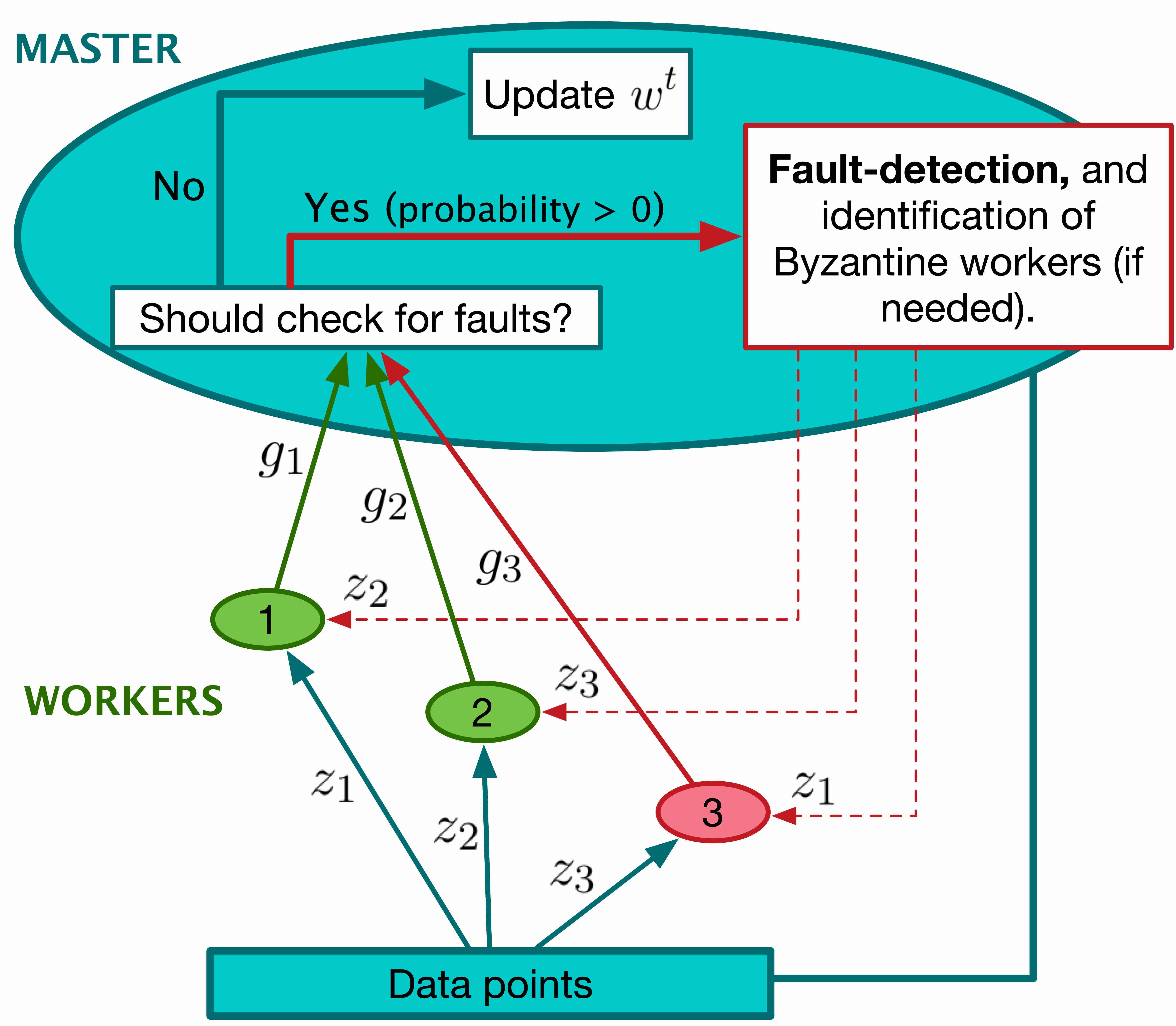
The master checks for faults only in intermittent iterations chosen at random, instead of all the iterations. Alternately, in each iteration, the master does a fault-check with some non-zero probability less than $1$. By doing so, the master significantly reduces the redundancy in gradients’ computations whilst almost surely identifying the Byzantine workers that send faulty symbols eventually²² 2 As the parallelized-SGD method converges to the learning parameter regardless of the initial parameter estimate, a Byzantine worker that eventually stops sending faulty gradients poses no harm to the learning process. Hence, the master only needs to identify Byzantine workers that send faulty gradient(s) eventually.. As in the deterministic scheme, upon detecting any fault(s) the master imposes reactive redundancy to identify the responsible Byzantine worker(s). However, correcting the detection fault(s) is optional. The identified Byzantine worker(s) are eliminated from the subsequent iterations.

An illustration of the scheme is presented in Figure 3. Additional details for the generic case is presented in Section 4.2.

Significant savings on redundancy: By reducing the probability of random fault-checks, the expected computation efficiency of the scheme can be made as close to $1$ as desirable. Note, a coding scheme that obtains exact fault-tolerance against a non-zero number of Byzantine workers cannot have an expected computation efficiency of $1$.

We note the following generalizations, and adaptation of the randomized scheme:

• •

  Generalization:

  • –

    Obviously, as in the deterministic case, the randomized scheme can be easily generalized for compressed gradients.

  • –

    Instead of checking for faults for all the workers with equal probability, the master may use different probabilities for different workers. For doing so, workers can be assigned reliability scores as in the context of reliable crowdsourcing [18]. Other generalizations are presented in Section 5.

• •

  Adaptation: A lower probability of fault-checks implies higher probability of using faulty gradients for parameter update, and vice-versa. Higher probability of faulty updates means higher probability of slower convergence of the learning algorithm. To manage the trade-off between the computation efficiency and the rate of learning, we present an adaptive approach in Section 4.3. Essentially, the master may vary the probability of fault-checks – depending upon the observed average loss at the current parameter estimate.

As an example of the deterministic scheme, we use a replication code. For simplicity, suppose that none of the Byzantine workers have been identified until iteration $t\geq 0$. Then, the scheme for the $t$-iteration is as follows.

The master (randomly) chooses $m$ data points, and assigns each data point to $f+1$ workers. Thus, each worker, on average, gets $m(f+1)/n$ data points. Upon computing the gradients for all its data points (at $w^{t}$), each worker sends a symbol; a tuple of its computed gradients. Consequentially, the master receives $f+1$ copies (or replicas) of each data point’s loss function’s gradient. As there are at most $f$ Byzantine workers, the master can detect if the received copies of a gradient are faulty by simply comparing them with each other. Suppose that the copies of the gradient of a particular data point $\hat{z}$ are faulty (i.e. they are not unanimous). Then, the master imposes reactive redundancy where it re-assigns $\hat{z}$ to $f$ additional workers that compute and send additional $f$ copies of the gradient for $\hat{z}$. Upon acquiring $2f+1$ copies of $\hat{z}$’s gradient, the master can not only obtain the correct gradient by majority voting, it also identify the responsible Byzantine worker(s). Ultimately, the master recovers the correct gradients for all the $m$ data points, and updates $w^{t}$ as (1).

The identified Byzantine worker(s) are eliminated from the subsequent iterations. Upon updating $f$ and $n$, the above scheme is repeated for the $(t+1)$-iteration.

In the randomized scheme, the master checks for faults (and does identification of Byzantine worker if needed) only for randomly chosen intermittent iterations. In each iteration, the master runs the traditional parallelized-SGD method by default. However, before updating the parameter estimate, the master decides to check for faults in the received symbols (or gradients) with probability $q>0$. Fault-checks and identification of Byzantine workers (if needed) is done using the protocol outlined for the deterministic coding scheme in Section 4.1.

For the purpose of analysis, assume that each Byzantine worker $i$ tampers its gradient(s) independently in each iteration with probability at least $p_{i}>0$. Then, $i$ remains unidentified by the master after $t$ iterations with probability less than or equal to $\left(1-{q\,p_{i}}\right)^{t}$, which approaches $0$ as $t$ approaches $\infty$. In other words, $i$ gets identified almost surely. This holds for all Byzantine workers that tamper gradient(s) eventually.

Let $\mathsf{comEff}_{t}(q)$ and $\mathsf{probF}_{t}(q)$ denote the expected computation efficiency and the probability of faulty update in iteration $t$, if the probability of doing a fault-check equals $q$. Let $\kappa_{t}$ denote the number of identified Byzantine workers until iteration $t$. By substituting $f$ by

in (2) and (3), we obtain

Note, maximizing $\mathsf{comEff}_{t}(q)$ is equivalent to minimizing $(1-\mathsf{comEff}_{t}(q))^{2}$, and minimizing $\mathsf{probF}_{t}(q)$ is equivalent to minimizing $(\mathsf{probF}_{t}(q))^{2}$. Thus, the probability of fault-check in the $t$-iteration, denoted by $q^{*}_{t}$, is given by the minimum point of the weighted average of $(1-\mathsf{comEff}_{t}(q))^{2}$ and $(\mathsf{probF}_{t}(q))^{2}$, i.e.,

where $\lambda_{t}\in[0,\,1]$. Higher value of $\lambda_{t}$ (greater than $1/2$) implies that minimizing $\mathsf{probF}_{t}(q)$ takes precedence over maximising $\mathsf{comEff}_{t}(q)$, and vice versa.

References

- [1] Alham Fikri Aji and Kenneth Heafield. Sparse communication for distributed gradient descent. arXiv preprint arXiv:1704.05021, 2017.
- [2] Jeremy Bernstein, Yu-Xiang Wang, Kamyar Azizzadenesheli, and Anima Anandkumar. signsgd: Compressed optimisation for non-convex problems. arXiv preprint arXiv:1802.04434, 2018.
- [3] Peva Blanchard, Rachid Guerraoui, Julien Stainer, et al. Machine learning with adversaries: Byzantine tolerant gradient descent. In Advances in Neural Information Processing Systems, pages 119–129, 2017.
- [4] Léon Bottou, Frank E Curtis, and Jorge Nocedal. Optimization methods for large-scale machine learning. Siam Review, 60(2):223–311, 2018.
- [5] Lingjiao Chen, Hongyi Wang, Zachary Charles, and Dimitris Papailiopoulos. DRACO: Byzantine-resilient distributed training via redundant gradients. In International Conference on Machine Learning, pages 903–912, 2018.
- [6] Yudong Chen, Lili Su, and Jiaming Xu. Distributed statistical machine learning in adversarial settings: Byzantine gradient descent. Proceedings of the ACM on Measurement and Analysis of Computing Systems, 1(2):44, 2017.
- [7] Deepesh Data, Linqi Song, and Suhas Diggavi. Data encoding for Byzantine-resilient distributed gradient descent. In 2018 56th Annual Allerton Conference on Communication, Control, and Computing (Allerton), pages 863–870. IEEE, 2018.
- [8] Ilias Diakonikolas, Gautam Kamath, Daniel M Kane, Jerry Li, Jacob Steinhardt, and Alistair Stewart. SEVER: A robust meta-algorithm for stochastic optimization. arXiv preprint arXiv:1803.02815, 2018.
- [9] Julie S Downs, Mandy B Holbrook, Steve Sheng, and Lorrie Faith Cranor. Are your participants gaming the system?: screening mechanical turk workers. In Proceedings of the SIGCHI conference on human factors in computing systems, pages 2399–2402. ACM, 2010.
- [10] Nirupam Gupta and Nitin H Vaidya. Byzantine fault-tolerant distributed linear regression. arXiv preprint arXiv:1903.08752, 2019.
- [11] Nirupam Gupta and Nitin H Vaidya. Byzantine fault-tolerant parallelized stochastic gradient descent for linear regression. 57th Annual Allerton Conference on Communication, Control, and Computing, 2019.
- [12] Srikanth Jagabathula, Lakshminarayanan Subramanian, and Ashwin Venkataraman. Identifying unreliable and adversarial workers in crowdsourced labeling tasks. Journal of Machine Learning Research, 18(93):1–67, 2017.
- [13] Yehuda Lindell. Introduction to coding theory lecture notes. Department of Computer Science Bar-Ilan University, Israel January, 25, 2010.
- [14] El Mahdi El Mhamdi, Rachid Guerraoui, and Arsany Guirguis. Fast machine learning with byzantine workers and servers. arXiv preprint arXiv:1911.07537, 2019.
- [15] Dhiraj K. Pradhan and Nitin H. Vaidya. Roll-forward and rollback recovery: Performance-reliability trade-off. IEEE Trans. Computers, 46(3):372–378, 1997.
- [16] Adarsh Prasad, Arun Sai Suggala, Sivaraman Balakrishnan, and Pradeep Ravikumar. Robust estimation via robust gradient estimation. arXiv preprint arXiv:1802.06485, 2018.
- [17] Shashank Rajput, Hongyi Wang, Zachary Charles, and Dimitris Papailiopoulos. DETOX: A redundancy-based framework for faster and more robust gradient aggregation. In Advances in Neural Information Processing Systems, pages 10320–10330, 2019.
- [18] Vikas C Raykar and Shipeng Yu. Eliminating spammers and ranking annotators for crowdsourced labeling tasks. Journal of Machine Learning Research, 13(Feb):491–518, 2012.
- [19] Navjot Singh, Deepesh Data, Jemin George, and Suhas Diggavi. SPARQ-SGD: Event-triggered and compressed communication in decentralized stochastic optimization. arXiv preprint arXiv:1910.14280, 2019.
- [20] Hanlin Tang, Xiangru Lian, Tong Zhang, and Ji Liu. Doublesqueeze: Parallel stochastic gradient descent with double-pass error-compensated compression. arXiv preprint arXiv:1905.05957, 2019.
- [21] Jeroen Vuurens, Arjen P de Vries, and Carsten Eickhoff. How much spam can you take? an analysis of crowdsourcing results to increase accuracy. In Proc. ACM SIGIR Workshop on Crowdsourcing for Information Retrieval (CIR’11), pages 21–26, 2011.
- [22] Rand R Wilcox. Introduction to robust estimation and hypothesis testing. Academic press, 2011.
- [23] Dong Yin, Yudong Chen, Kannan Ramchandran, and Peter Bartlett. Byzantine-robust distributed learning: Towards optimal statistical rates. In International Conference on Machine Learning, pages 5636–5645, 2018.
- [24] Martin Zinkevich, Markus Weimer, Lihong Li, and Alex J Smola. Parallelized stochastic gradient descent. In Advances in neural information processing systems, pages 2595–2603, 2010.