Multi-Robot Path Planning Via Genetic Programming
Abstract
This paper presents a Genetic Programming (GP) approach to solving multi-robot path planning (MRPP) problems in single-lane workspaces, specifically those easily mapped to graph representations. GP’s versatility enables this approach to produce programs optimizing for multiple attributes rather than a single attribute such as path length or completeness. When optimizing for the number of time steps needed to solve individual MRPP problems, the GP constructed programs outperformed complete MRPP algorithms, i.e. Push-Swap-Wait (PSW), by . The GP constructed programs also consistently outperformed PSW in solving problems that did not meet PSW’s completeness conditions. Furthermore, the GP constructed programs exhibited a greater capacity for scaling than PSW as the number of robots navigating within an MRPP environment increased. This research illustrates the benefits of using Genetic Programming for solving individual MRPP problems, including instances in which the number of robots exceeds the number of leaves in the tree-modeled workspace.
Keywords:
Multi-robot path planning Genetic programming.1 Introduction
Multi-robot systems offer greater performance than single robot systems at the cost of addressing issues, including the potential for collisions, bottlenecks, and traffic jams that can occur when many robots are navigating within confined or single-lane environments. To address such issues, the problem of Multi-Robot Path Planning (MRPP) has been explored within many contexts, e.g. [3, 7, 10]. A solution to the MRPP problem typically requires the construction of a collision-free path for each robot having a unique starting location and unique goal location within the workspace. In solving this problem, researchers have focused on developing algorithms that are scalable, complete, and/or optimal (e.g. with respect to path length) [4, 14, 16, 20, 21, 23].

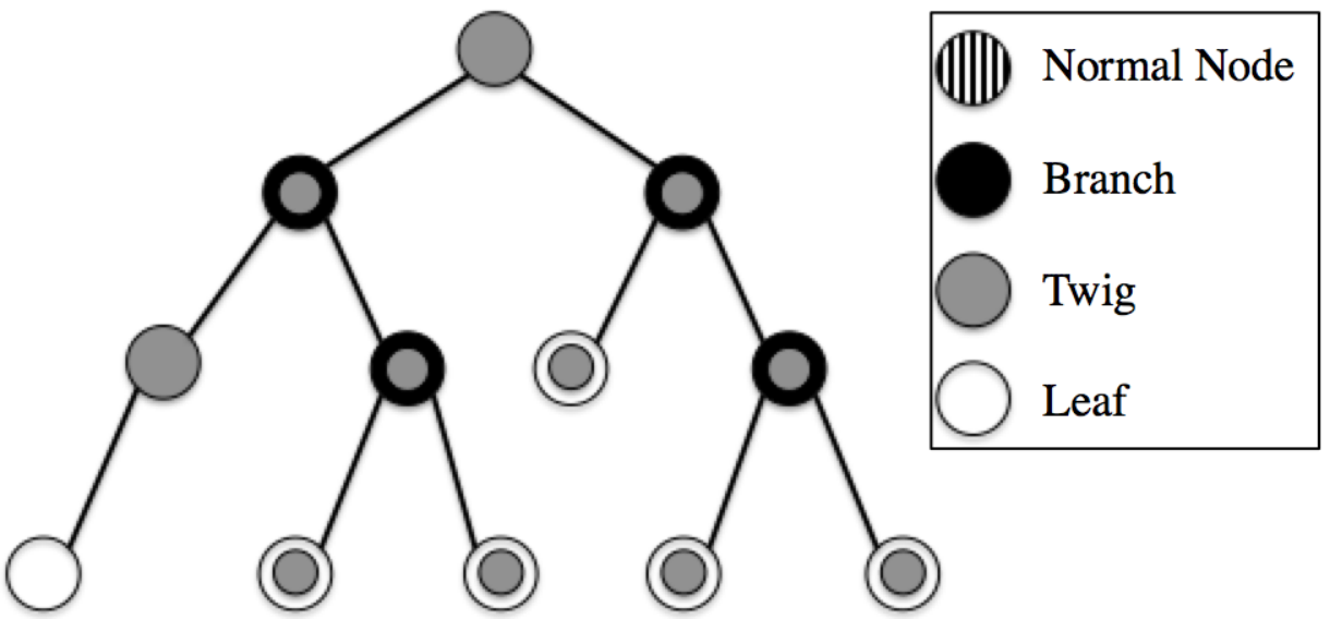
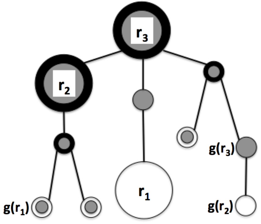
This paper focuses on MRPP within the single-lane environments typically found in mines and warehouses. In these workspaces, fleets of autonomous robots navigate single lane tunnels; for example, in Fig. 1(a), the robots do not have space to move around each other safely. As in previous work, this research abstracts such workspaces as minimum spanning trees (see Fig. 1(b)), in which robot actions correspond to movement along edges connecting nodes [24].
This paper presents a Genetic Programming (GP) approach to single-lane MRPP. GP is an evolutionary algorithm that evolves computer programs as solutions to problems. Here, a centralized master computer first runs the GP algorithm offline on a training set of MRPP examples, learns a computer program that solves these examples, and shares this program with the robots within the environment. Then, the robots sequentially execute the learned program in real-time to determine their next actions. Each robot runs this computer program at each time step until all of the robots have visited their respective goal destinations. The specific contributions of this paper include:
- 1.
Identification of a set of GP functions and terminals for generating MRPP programs.
- 2.
A GP algorithm for constructing programs solving MRPP problems.
- 3.
Simulation results illustrating GP performance in solving single MRPP instances and in developing a general MRPP program.
In Section 2, MRPP/GP related research is introduced. Section 3 provides the problem formulation. In Section 4, a GP algorithm is outlined and its application to MRPP explained. In Section 5, the computational complexity of the GP algorithm is evaluated. Section 6 describes how the GP’s function set and terminal set were developed. Section 7 documents the experiments performed to validate the approach. In Section 8, conclusions are presented and future work is considered.
2 Background
MRPP algorithms can be classified in multiple ways. First, they can be classified as centralized or decentralized. Centralized MRPP algorithms have a single robot or central computer plan the paths of all the robots [4, 14, 16, 20]. Decentralized MRPP algorithms have each individual robot plan its own path [2, 7, 15, 22, 29]. MRPP algorithms can also be distinguished by whether they are local or global. Local MRPP algorithms determine a robot’s next move at each time step whereas global MRPP algorithms generate a robot’s entire path before it sets off towards its destination.
Related to multi-robot path planning in graphs is the work on pebble motion. A pebble motion algorithm aiming to move pebbles around a tree from a start to goal configuration is shown in [1]. Earlier work also includes [12]. More recent work [28] presents an algorithm that upper bounds the number of moves required for moving pebbles around a graph to their goal configuration. Finally, a polynomial time algorithm for coordinating the motion of labeled discs in high disc density scenarios [6] is shown to have optimality guarantees.
Recent centralized MRPP approaches include [8], a polynomial time algorithm (SEAR) with expected optimality guarantees in obstacle-free environments. In [27], MRPP algorithms for optimizing across several metrics (e.g. makespan, max distance, etc.) are shown to calculate near optimal paths for 100+ robots in seconds. Other work [17] aims to maximize the number of agents that can reach their goal under a deadline.
Presented in [24], the Push-Swap-Wait algorithm (PSW) is a decentralized, local, and topology-based single-lane MRPP algorithm that distinguishes itself from other MRPP algorithms in that it is complete: it is guaranteed to solve MRPP problems that meet certain conditions. Unlike most multi-agent path finding approaches, however, PSW considers an environment solved once each robot has visited its unique destination. Under this definition, robots do not need to remain at their destination once solved. Centralized and complete MRPP algorithms have also been developed [20].
GP has been successfully used to evolve collision avoidance programs for single robots. The collision avoidance programs generated by the GP in [19] are structured as trees containing arithmetic and boolean operators. The programs take in robot sensor readings and return motor speeds.
GP has also been used in MRPP. Kala used Grammar Guided Genetic Programming (GGGP) to evolve optimal paths for individual MRPP examples [11]. For a given instance of MRPP, GGGP is run for each robot so that they learn the best paths to their respective destinations. A master genetic algorithm then optimizes across robots, selecting the path for each robot ensuring that the robots collectively reach their destinations as quickly as possible without colliding.
Evolutionary algorithms other than GP have been used in MRPP. In [18] and [26], Cooperative Co-evolution is used to generate paths that achieve collision avoidance in individual MRPP examples. Here, the entities undergoing evolution are the paths themselves, which is useful in producing environment specific optimal paths. Chakraborty, Konar, Jain, & Chakraborty use Differential Evolution to generate algorithms for MRPP [5]. In this approach, each robot has its own path-planning algorithm that evolves. Lastly, Das, Sahoo, Behera, & Vashisht use Particle Swarm Optimization to generate decentralized and local algorithms for MRPP [9].
This paper presents a decentralized, local, and topology-based GP approach to single-lane MRPP. The performance of this approach is compared to PSW. Similarly to PSW, an environment is considered solved once each robot has visited its destination. Unlike PSW and the evolutionary algorithms mentioned above, the GP approach presented in this paper is the first research we know of that constructs decentralized and scalable single-lane MRPP programs using GP.
3 Problem Formulation
This research attempts to develop a GP algorithm that can be run offline to construct a solution program to be downloaded to multiple individual robots (see Fig. 2). Then, each robot can execute to enable collision-free, decentralized navigation through a given single-lane workspace to its goal destination.

In designing the GP algorithm that constructs , it is assumed that the navigable portions of the workspace are modeled as a fully connected graph, which can in turn be represented with a minimum spanning tree , composed of a set of nodes, , connected with a set of undirected edges, . Recall that a minimum spanning tree of graph contains the same set of nodes and contains a subset of the edges such that all of the nodes remain connected and there are no cycles. The tree is occupied by a set of robots that are assumed to travel at the same constant speed. Each robot may traverse an edge during a time step and must occupy a node at the end of a time step. Only a single robot may occupy a given node at a time.
At each time step , each robot runs the GP generated program , which returns the robot’s assignment . Thus, if and , robot traverses edge during time step if and . Each edge is of the same length and takes a single time step to traverse. An edge can only be traversed by a single robot during a given time step. Each robot starts on a unique starting node such that if . Each robot also has a unique destination node such that if .
All robots within nodes of in the minimum spanning tree are considered to be in ’s direct communication network: .
Finally, a MRPP problem is considered solved at time if and . In other words, a MRPP problem is considered solved once each robot has visited its destination node.
4 Genetic Programming in MRPP
Genetic Programming is an evolutionary algorithm that begins with an initial, randomly generated population of solution programs. These programs are iteratively tested against a set of training examples to evaluate their fitness—how well they solve the training problems.
| Function | Description |
|---|---|
| If-Two-Robots-On-Each-Others-Path | Checks whether the current robot ’s position is on the path of another robot that belongs to . Also checks whether is on ’s path. If both conditions are met, and each set their paths to the nearest branch node to . |
| If-Neighbor-Is-Surrounded | Checks whether the current robot is adjacent to another robot that is surrounded—that is, each of ’s adjacent nodes are occupied by a robot. |
| If-Robot-At-Branch | Checks whether the current robot is at a branch node that it set its path to. |
| If-Robot-At-Destination | Checks whether the current robot is at its destination node . |
| If-Robot-Moving-To-Branch | Checks whether the current robot is travelling to a branch node it has set its path to but hasn’t reached yet. |
| If-Neighbor-On-Path-Is-Free | Checks whether the next node on the current robot ’s path is free. |
| If-Robot-Is-Solved | Checks whether the current robot has visited its destination node . |
| If-On-Path-Of-Robot-In-Network | Checks whether the current robot ’s position is on the path of another robot that belongs to its direct communication network . |
| If-Robot-In-Network-Moving-To-Branch | Checks whether a robot that belongs to is travelling to a branch node. |
The next generation of programs is then produced via asexual reproduction, genetic crossover, and mutation, whereby more fit solutions are granted a greater likelihood of surviving the evolutionary process. This leads the population of solutions to become increasingly fit over the course of generations [13].
4.1 Solution Representation
GP solutions are computer programs that are structured as trees. The internal nodes in the tree-structured programs are sampled from the function set , where a function can be an arithmetic/boolean/conditional operator, mathematical/iterative/recursive function, etc. Here, includes conditional if-statements relying on information about the environment: e.g. the positions of robots relative to other robots, the positions of robots relative to branch nodes, etc. (see Table 1). Whenever a function or terminal requires the current robot to compute a path from its current node to its destination node or to a branch node, Dijkstra’s algorithm is used. To note, a branch node is a node in the minimum spanning tree having 3 or more neighbors.
The leaves in the computer program’s tree structure are sampled from the terminal set and can be constants, variables, or functions changing the state of the environment. The terminals used here are actions dictating a robot’s movement between nodes in the workspace (see Table 2). Each of the terminals contain a block of code that checks whether execution of the terminal would result in a collision. If a robot executes a terminal that would cause it to travel to a node that is already occupied by another robot, this block of code ensures that the robot stays at its current node in order to prevent a collision.
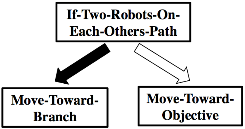
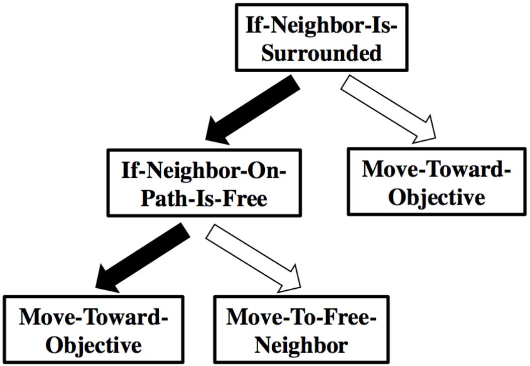
Given the programs’ internal nodes are conditional operators, the resulting solution programs represent decision trees solving MRPP problems (e.g. Fig. 3a-b).
| Terminal | Description |
|---|---|
| Move-Toward-Branch | The current robot moves to the next node on the path to the branch it has set its path to. |
| Move-To-Free-Neighbor | The current robot moves to an adjacent node that isn’t occupied by a robot and that it hasn’t visited before. |
| Move-Toward-Objective | The current robot moves to the next node on its current path. |
| Stay | The current robot does not move during the time step and stays at the same node. |
4.2 GP Algorithm
Inputs: , , , , , ,
In Alg. 1, the GP evolves solution programs solving MRPP problems over the course of runs, each lasting generations. At the start of each run, is executed (line 4), randomly generating an initial population of programs, with maximum tree depth 2, composed of the functions and terminals from Table 1 and Table 2. Then, for each generation within the given run, the GP iterates through each program in the population and executes (line 7). This function runs a given program against a set of MRPP training problems . The time it takes program to solve training problem is recorded for all programs in over all examples in . If a program solves all of the examples in in fewer time steps than the current best program , then the minimum number of time steps taken to solve the examples in , , is updated (line 9) and becomes the new best program (line 10). At the end of each generation, the next generation’s population of programs is produced by running with asexual reproduction rate (line 13), with genetic crossover rate (line 14), and with mutation rate (line 15). , , and define the proportion of programs in the next generation that come from asexual reproduction, genetic crossover, and mutation, respectively. Thus, , , and must sum to 1 so that is constant over the generations. This iterative process continues for runs of generations. Once the final run has ended, the best solution program is returned (line 19).
4.3 Calculating Fitness
To evaluate the quality of a program , it is tested against a set of examples called the fitness set: . Each example is a randomly generated MRPP problem including a minimum spanning tree and a set of robots having unique starting and destination nodes.
Notably, a program is tested against each example until the example has been solved or the maximum allowable time steps has been exceeded, where , is the number of nodes in , and is the number of robots. The fitness function to be is defined as .
Specifically, program ’s fitness for training problem is:
| (1) |
where returns the number of edges along the shortest path from to at time . A training problem can be considered solved but not have because a problem is considered solved once each robot has visited its destination. Robots do not need to remain at their destinations once they have been visited.
To evolve MRPP programs navigating robots to their destination nodes in as few time steps as possible, the fitness function calculation only allows a candidate program a total of time steps to solve all of the examples in . As the GP evolves, is updated to be the minimum number of time steps that has been found to solve (line 9).
4.4 Generating New Populations
Once the fitness score has been calculated for each program in the population, the next generation’s population of programs is created— from asexual reproduction, from genetic crossover, and from mutations. Programs are selected to undergo these operations with fitness proportionate probability , where .
Asexual Reproduction
Each program is copied from the current population into the new population with probability .
Genetic Crossover
Two programs from the current population are chosen with fitness proportionate probabilities. Then, a crossover point (i.e. a node) is randomly chosen in both program’s decision trees. The subtrees at the crossover points are then swapped and reattached at the crossover points to form two new programs (e.g. Fig. 3c-d) that are added to the new population.
Mutation
A program from the current population is selected with probability . Then, as in genetic crossover, a node in the program’s decision tree is uniformly randomly chosen. The chosen node and its subtree are deleted and replaced with a randomly generated subtree (e.g. Fig. 3d).


5 Computational Complexity
The genetic program returns a single path planning program that is used by each robot within the environment. At each time step, the robots in the environment sequentially call to determine their next action. As previously discussed, has the form of a decision tree. An input parameter to the GP construction algorithm is , dictating the maximum depth of . Thus, when a robot calls and does a traversal of the decision tree, it traverses a single branch that consists of at most nodes. This means that at most functions and 1 terminal are executed by each robot each time step.
To determine the computational complexity of having a single robot call in a given time step, the most expensive function and terminal must be established because in the worst case, the most expensive function will be executed times and the most expensive terminal will be executed once. The most expensive function is If-Two-Robots-On-Each-Others-Path and the most expensive terminal is Move-Toward-Branch.
If-Two-Robots-On-Each-Others-Path has computational complexity , where is the maximum branching factor in the tree and all robots within nodes of a robot in are considered to be in ’s direct communication network: . The term comes from having to construct the current robot’s direct communication network . If two robots are on each other’s paths, then the nearest branch node is found. This requires Dijkstra’s algorithm to be called between ’s current position and each branch node. The computational complexity of Dijkstra’s algorithm is where and are the number of edges and nodes in the graph, respectively. Since the algorithm is being executed on a tree, . Thus, the computational complexity of Dijkstra’s algorithm can be rewritten as . The number of branch nodes is upper bounded by the number of nodes . Therefore, finding the closest branch node to has complexity .
Move-Toward-Branch also has computational complexity , deriving from the requirement of finding the closest branch node to the current robot .
In , the maximum branching factor is typically much smaller than and in our experiments, was set to 2. Therefore, . This leads us to conclude that the computational complexity of If-Two-Robots-On-Each-Others-Path and Move-Toward-Branch are each
. The computational complexity of executing once is, therefore, or .
6 Developing the Function and Terminal Sets
Developing the GP’s function and terminal sets and for solving MRPP problems involved two phases. In phase one, functions and terminals enabling robots to swap positions were identified, a key requirement for removing deadlock in tunnel environments. The three unique MRPP scenarios requiring a swap were enumerated in [25]. These scenarios have been adapted and described in terms of robots and here:
- 1.
is on the path from to and is on the path from to
- 2.
Both and are on the path from to
- 3.
is on the path from to and ’s neighbors are all occupied by other robots
These three scenarios were encoded in to train the GP. The sets and were fine-tuned until the GP was able to find solution programs.
In phase two, function set and terminal set were further fine-tuned until the GP was capable of consecutively solving 100 randomly generated MRPP problems, each including a randomly constructed minimum spanning tree, occupied by a random number of robots having unique start and goal locations. To note, the number of robots was always fewer than the number of tree leaves (e.g. Fig. 1c). The final function set and terminal set can be found in Table 1 and Table 2, respectively.
7 Experiments
Three sets of experiments were conducted to evaluate GP’s ability to generate programs for solving MRPP problems. The first set of experiments tested GP’s ability to evolve programs for solving individual MRPP problems in the fewest possible time steps. The second set evaluated GP’s capacity to evolve general programs for solving problems they were not trained on. The third set tested GP’s ability to solve MRPP problems where PSW is not guaranteed to work.
In each experiment, a master computer first ran the GP algorithm offline on a fitness set of MRPP training examples. The GP algorithm was implemented using the EpochX Java library and was run on a Microsoft Surface Book with an Intel Core i7-6600U 71 CPU. The GP used a genetic crossover rate of , an asexual reproduction rate of , and a mutation rate of . Additionally, the algorithm ran for runs of generations. The population size was set to . The program tree depths were bounded between 1 and 50. After the last run, the GP algorithm returned the learned program . Then, for each test problem, was shared with each of the robots and executed online, in real-time, (as illustrated in Fig. 2). The robots sequentially executed every time step to determine their next action until the problem was solved or the maximum number of allowable time steps had been reached.
In the plots below, each data point is the average y-value across examples sharing an x-value. Error bars represent the standard deviation of the y-value.
7.1 Generating Training and Test Examples
Training and test examples were recursively created with the same random minimum spanning tree (MST) generator shown in Algorithm 2. The generator was provided seed values between 4 and 10 to produce training examples and seed values between 4 and 9 to produce test examples. The maximum branching factor was set to 4. Once the MST was generated, it was populated with robots, each having a unique, random starting node and destination node. In the experiments described in sections 7.2 and 7.3, the number of robots was set to because this is the maximum number of robots for which PSW is guaranteed to solve an environment. In section 7.4, the number of robots was set to , , , and times the number of leaf nodes.
7.2 Optimizing for Time in Individual MRPPs
GP programs were evolved to solve individual randomly generated MRPP examples in the fewest possible time steps. This process was conducted 1000 times. PSW was run against the same 1000 problems for comparison.
| GP Better | GP = PSW | PSW Better |
| 73.3 | 12.1 | 14.6 |
The results presented in Table 3 show that GP outperformed or tied PSW in of the trials. Furthermore, PSW required 18633 time steps to solve the 1000 examples while GP only needed 8552 time steps to solve the 1000 examples, a improvement. Fig. 4 suggests that GP increasingly outperforms PSW as the number of robots navigating within an environment increases. Fig. 5 reveals that GP increasingly outperforms PSW as the swaps/ robots ratio increases. In solving individual MRPP problems, then, GP significantly outperforms PSW and GP exhibits a greater capacity to scale as the number of robots navigating within an environment increases.


7.3 Generalizing GP to Solve New MRPPs
GP’s capacity to evolve general MRPP programs for solving new problems, on which they were not trained, is examined next. Trials were conducted where the GP evolved based on a set of = 5, 10, or 20 randomly generated training problems. Next, the learned program was run against a test set of 100 randomly generated MRPP examples. This process was repeated ten times for each value (yielding 1000 examples for each ) and the results are presented in Table 4.
These experiments reveal that GP’s ability to produce general programs improves as increases. Despite the improvement, GP was not able to match PSW’s completeness guarantee. Furthermore, in the problems solved by GP, increasing did not help GP outperform PSW as the percentage of examples in which GP required fewer time steps remained stable between and . Fig. 6 reveals that PSW consistently outperforms GP programs over all problem sizes. However, Fig. 7 suggests that general GP programs outperform PSW when robots must, on average, perform more swaps.


| GP Solved | GP Better | GP = PSW | PSW Better | |
| 5 | 695 | 36.69 | 11.65 | 51.65 |
| 10 | 866 | 30.37 | 15.24 | 54.39 |
| 20 | 872 | 32.80 | 11.12 | 56.08 |
| Leaf Multiplier | GP Solved | PSW Solved |
|---|---|---|
| 0.25 | 100 | 100 |
| 0.5 | 100 | 100 |
| 1.0 | 82 | 68.5 |
| 1.5 | 58 | 34 |
7.4 GP vs. PSW Where PSW Is Not Complete
GP’s ability to evolve programs solving individual MRPP problems violating PSW’s completeness guarantee—examples where —is examined next. Here, 200 trials were conducted in which the number of robots was fixed at , where was set to 0.25, 0.5, 1.0, and 1.5, respectively. In each trial, a GP program was evolved to solve an individual randomly generated MRPP example and PSW was run against the same problem for comparison. If , was set to because at least two nodes must be free to enable a swap. In the trials in which PSW’s completeness guarantee was in effect, both PSW and GP were able to find solutions of the time (see Table 5). When PSW’s completeness guarantee was violated ( and ), GP consistently solved more examples than PSW, e.g. solving more examples when .
8 Conclusions and Future Work
This paper presents a decentralized, local GP approach for solving single-lane MRPP problems. This GP approach facilitates the generation of MRPP programs that can optimize for various attributes and scenarios. GP effectively optimizes the number of time steps needed to solve individual MRPP problems, showing significant improvement over complete algorithms like PSW. GP also consistently outperforms PSW in solving problems that do not meet PSW’s completeness conditions. Furthermore, GP exhibits a greater capacity than PSW to scale as the number of robots navigating within an MRPP environment increases. This research illustrates the benefits of using GP to generate solutions for individual MRPP problems, including instances in which the number of robots exceeds the number of leaves in the tree-modeled workspace. However, attempts to use GP to produce general MRPP programs could not match PSW’s completeness despite the suggestion that general GP programs do outperform PSW where robots must perform more swaps. Future work should focus on developing functions and terminals enabling GP to produce more general MRPP programs and programs that better optimize for time. Additional experiments should reduce the constraints on the environment by training and testing on general graphs rather than MSTs. Furthermore, future research should attempt to modify this GP framework so that the learned program can be executed asynchronously within the environment. Finally, the programs produced by GP should be implemented on physical robots to better understand the nature of these programs and to observe where there is room for improvement.
References
- [1] Auletta, V., Monti, A., Parente, M., Persiano, P.: A linear-time algorithm for the feasibility of pebble motion on trees. Algorithmica 23(3), 223–245 (Mar 1999). https://doi.org/10.1007/PL00009259
- [2] Ayanian, N., Kumar, V.: Decentralized feedback controllers for multi-agent teams in environments with obstacles. In: 2008 IEEE International Conference on Robotics and Automation. pp. 1936–1941 (May 2008). https://doi.org/10.1109/ROBOT.2008.4543490
- [3] Cao, Y.U., Fukunaga, A.S., Kahng, A.: Cooperative mobile robotics: Antecedents and directions. Autonomous Robots 4(1), 7–27 (Mar 1997). https://doi.org/10.1023/A:1008855018923
- [4] Carpin, S., Pagello, E.: On parallel rrts for multi-robot systems. In: Proc. 8th Conf. Italian Association for Artificial Intelligence. pp. 834–841 (2002)
- [5] Chakraborty, J., Konar, A., Jain, L., Kumar Chakraborty, U.: Cooperative multi-robot path planning using differential evolution. Journal of Intelligent and Fuzzy Systems 20, 13–27 (01 2009). https://doi.org/10.3233/IFS-2009-0412
- [6] Chinta, R., Han, S.D., Yu, J.: Coordinating the motion of labeled discs with optimality guarantees under extreme density. CoRR abs/1807.03347 (2018), http://algorithmic-robotics.org/wafr2018/ppr_files/WAFR_2018_paper_6.pdf
- [7] Clark, C.: Dynamic Robot Networks: A Coordination Platform for Multi-Robot Systems. Ph.D. thesis, Stanford University (2004)
- [8] D. Han, S., J. Rodriguez, E., Yu, J.: Sear: A polynomial- time multi-robot path planning algorithm with expected constant-factor optimality guarantee. In: IEEE/RSJ International Conference on Intelligent Robots and Systems. pp. 1–9 (10 2018). https://doi.org/10.1109/IROS.2018.8594417
- [9] Das, P.K., Sahoo, B.M., Behera, H.S., Vashisht, S.: An improved particle swarm optimization for multi-robot path planning. In: 2016 International Conference on Innovation and Challenges in Cyber Security (ICICCS-INBUSH). pp. 97–106 (Feb 2016). https://doi.org/10.1109/ICICCS.2016.7542324
- [10] Dudek, G., Jenkin, M.R.M., Milios, E., Wilkes, D.: A taxonomy for multi-agent robotics. Autonomous Robots 3(4), 375–397 (Dec 1996). https://doi.org/10.1007/BF00240651
- [11] Kala, R.: Multi-robot path planning using co-evolutionary genetic programming. Expert Syst. Appl. 39(3), 3817–3831 (Feb 2012). https://doi.org/10.1016/j.eswa.2011.09.090
- [12] Kornhauser, D., Miller, G., Spirakis, P.: Coordinating pebble motion on graphs, the diameter of permutation groups, and applications. In: 25th Annual Symposium on Foundations of Computer Science, 1984. pp. 241–250 (Oct 1984). https://doi.org/10.1109/SFCS.1984.715921
- [13] Koza, J.R.: Genetic Programming: On the Programming of Computers by Means of Natural Selection. MIT Press, Cambridge, MA, USA (1992)
- [14] Luna, R., Bekris, K.E.: Efficient and complete centralized multi-robot path planning. In: 2011 IEEE/RSJ International Conference on Intelligent Robots and Systems. pp. 3268–3275 (Sept 2011). https://doi.org/10.1109/IROS.2011.6095085
- [15] Luna, R.: Efficient multi-robot path planning in discrete spaces. Master’s thesis, University of Nevada (2011)
- [16] Luna, R., Bekris, K.E.: Push and swap: Fast cooperative path-finding with completeness guarantees. In: Proceedings of the Twenty-Second International Joint Conference on Artificial Intelligence - Volume Volume One. pp. 294–300. IJCAI’11, AAAI Press (2011). https://doi.org/10.5591/978-1-57735-516-8/IJCAI11-059, http://dx.doi.org/10.5591/978-1-57735-516-8/IJCAI11-059
- [17] Ma, H., Wagner, G., Felner, A., Li, J., Kumar, T.K.S., Koenig, S.: Multi-agent path finding with deadlines. In: Proceedings of the Twenty-Seventh International Joint Conference on Artificial Intelligence, IJCAI-18. pp. 417–423. International Joint Conferences on Artificial Intelligence Organization (7 2018). https://doi.org/10.24963/ijcai.2018/58
- [18] Mei, W., Tie-jun, W.: Cooperative co-evolution based distributed path planning of multiple mobile robots. Journal of Zhejiang University-SCIENCE A 6(7), 697–706 (Jul 2005). https://doi.org/10.1631/jzus.2005.A0697
- [19] Nordin, P., Banzhaf, W.: Real time control of a khepera robot using genetic programming. Cybernetics and Control 26, 533–561 (1997), http://citeseerx.ist.psu.edu/viewdoc/summary?doi=10.1.1.52.631
- [20] Peasgood, M., Clark, C.M., McPhee, J.: A complete and scalable strategy for coordinating multiple robots within roadmaps. IEEE Transactions on Robotics 24(2), 283–292 (April 2008). https://doi.org/10.1109/TRO.2008.918056
- [21] Standley, T., Korf, R.: Complete algorithms for cooperative pathfinding problems. In: Proceedings of the Twenty-Second International Joint Conference on Artificial Intelligence - Volume Volume One. pp. 668–673. IJCAI’11, AAAI Press (2011). https://doi.org/10.5591/978-1-57735-516-8/IJCAI11-118
- [22] Velagapudi, P., Sycara, K., Scerri, P.: Decentralized prioritized planning in large multirobot teams. In: 2010 IEEE/RSJ International Conference on Intelligent Robots and Systems. pp. 4603–4609 (Oct 2010). https://doi.org/10.1109/IROS.2010.5649438
- [23] Wang, K.H., Botea, A.: Mapp: a scalable multi-agent path planning algorithm with tractability and completeness guarantees. Journal of Artificial Intelligence Research 42, 55–90 (09 2011). https://doi.org/10.1613/jair.3370
- [24] Wiktor, A., Scobee, D., Messenger, S., Clark, C.: Decentralized and complete multi-robot motion planning in confined spaces. In: 2014 IEEE/RSJ International Conference on Intelligent Robots and Systems. pp. 1168–1175 (Sep 2014). https://doi.org/10.1109/IROS.2014.6942705
- [25] Wiktor, A., Scobee, D.: Decentralized and complete multi-robot motion planning in confined spaces (2012)
- [26] Yang, D., Chen, J., Matsumoto, N., Yamane, Y.: Multi-robot path planning based on cooperative co-evolution and adaptive cga. In: 2006 IEEE/WIC/ACM International Conference on Intelligent Agent Technology. pp. 547–550 (Dec 2006). https://doi.org/10.1109/IAT.2006.94
- [27] Yu, J., LaValle, S.M.: Optimal multirobot path planning on graphs: Complete algorithms and effective heuristics. IEEE Transactions on Robotics 32(5), 1163–1177 (Oct 2016). https://doi.org/10.1109/TRO.2016.2593448
- [28] Yu, J., Rus, D.: Pebble Motion on Graphs with Rotations: Efficient Feasibility Tests and Planning Algorithms, pp. 729–746. Springer International Publishing, Cham (2015). https://doi.org/10.1007/978-3-319-16595-0_42
- [29] Zheng, J., Yu, H., Liang, W., Zeng, P.: A distributed and optimal algorithm to coordinate the motion of multiple mobile robots. In: 2008 7th World Congress on Intelligent Control and Automation. pp. 3027–3032 (June 2008). https://doi.org/10.1109/WCICA.2008.4594486