QANOVA: Quantile-based Permutation Methods For General Factorial Designs

Factorial designs are popular in various fields such as ecology, biomedicine and psychology (GISSI-2 1990; Baigent et al. 1998; Cassidy et al. 2008; Mehta et al. 2010; Kurz et al. 2015) as they us allow to study interaction effects between different factors alongside their main effects. In fact, Lubsen and Pocock 1994 pointed out that “it is desirable for reports of factorial trials to include estimates of the interaction between the treatments”. The ANOVA-$F$-test is the most common tool for this but suffers from restrictive assumptions such as homoscedasticity and normality. Thus, several tests have been developed that allow for non-normal errors or are valid for heteroscedastic one- and two-way or even more general factorial designs (Johansen 1980; Brunner et al. 1997; Bathke et al. 2009; Zhang 2012; Pauly et al. 2015; Friedrich et al. 2017a; Friedrich et al. 2017b; Harrar et al. 2019).

All these procedures describe effects by (contrasts of) means. This is in line with a phenomenon observed in various areas: comparisons are mainly based upon means or variances but not on their robust counterparts. This can be explained in part by the simplicity and elegance gained by using linear or, under independence, additive statistics. Nevertheless it contradicts the important role of statistics based on quantiles, like the median and the interquartile range (IQR), in data exploration and modeling, e.g. in boxplots or summary statistics. The interest in analyzing quantiles has lead to the development of quantile regression, which is commonly established nowadays (Koenker and Hallock 2001; Koenker et al. 2019). However, as, e.g., stressed by Beyerlein 2014 “it appears to be quite underused in medical research”. One reason may be that, although there exist several approaches for specific designs (Sen 1962; Potthoff 1963; Fung 1980; Hettmansperger and McKean 2010; Fried and Dehling 2011; Chung and Romano 2013), there does not exist an equal abundance of methods based on quantiles for general factorial designs. There are procedures, at least for the median, but they often require strong distributional assumptions (as symmetry) or, at least, an extension to factorial designs is missing. Therefore the main aims of the present paper are to develop inference procedures (tests and compatible confidence regions)

• (i)

  for the median, the interquartile range (IQR) or any linear combination of quantiles.

• (ii)

  within the framework of factorial designs to study robust main and interaction effects.

• (iii)

  for general heterogeneous or heteroscedastic models beyond normality.

• (iv)

  that are theoretically valid and posses a satisfactory finite sample performance.

To achieve these goals, we combine and extend the ideas of Chung and Romano 2013 (who derive tests for equality of medians in one-way ANOVA models) and Pauly et al. 2015 (who establish mean-based testing procedures in general factorial designs) to (simultaneously) infer arbitrary linear contrasts of general quantiles. In view of (ii) and (iv) we thereby follow the idea of permuting studentized Wald-type statistics to obtain methods that are finitely correct in case of exchangeable data (e.g., under the null hypothesis of equal means / medians in the classic $F$-ANOVA normal model) but also asymptotically valid for general non-exchangeable settings. This alluring technique has originally been developed for special two-sample models (Neuhaus 1993; Janssen 1997; Janssen and Pauls 2003; Pauly 2011) and has recently displayed its full strength to obtain accurate methods in one-way (Chung and Romano 2013) and more general factorial designs (Pauly et al. 2015; Friedrich et al. 2017a; Smaga 2017; Umlauft et al. 2017; Harrar et al. 2019).

However, to derive the fore-mentioned theoretical evidence in our general quantile-based approaches we could not employ the methods derived in the previously mentioned papers. In fact, to overcome some technical difficulties that occur when jointly permuting sample quantiles, we had to take a detour in which we extended some results for general permutation empirical processes and uniform Hadamard differentiability (van der Vaart and Wellner 1996) that are of own mathematical interest. Anyhow, this finally results in (i)-(iv), i.e., a flexible toolbox for inferring contrasts of different quantiles in factorial designs. In the special case of the median and its bootstrap-based variance estimator we obtain the one-way permutation test derived in Chung and Romano 2013.

The paper is organized as follows: We first introduce the model, estimators for population quantiles and how to formulate null hypotheses in them to test for certain main or interaction effects. In Section 3, we state the theory to handle the joint asymptotics for sample quantiles and their covariance matrix estimators. As the latter are crucial to obtain the correct dependency structure necessary in the aforementioned studentization we study three different approaches based upon kernel density estimators, bootstrapping or certain interval estimates. As they are mostly only known for the sample median, these considerations require certain extension to our more general situations which are explained in Sections 3.1–3.2. From these findings we then deduce three different asymptotically valid testing procedures. To improve their small sample performance, we consider their respective permutation versions in Section 4, prove asymptotic exactness and also analyze their power under local and fixed alternatives. To compare the small sample behavior of the resulting six tests, we conducted extensive simulations presented in Section 5. Finally, we illustrate the new methodology by analyzing a recent data set on the height and weight of children in different countries in Section 6. All proofs are deferred to the appendix, where also some additional simulation results are presented.

We consider a general model given by mutually independent random variables

with absolutely continuous distribution functions $F_{i}$ and corresponding densities $f_{i}$. This set-up allows the incorporation of divers factorial structure by adequately splitting up indices. To accept this consider for example a two-way design with factors $A$ (possessing $a$ levels) and $B$ (having $b$ levels). Setting $k=a\cdot b$ we split up the group index $i$ into $i=(i_{1},i_{2})$ and model observations as $X_{i_{1}i_{2}j}\sim F_{i_{1}i_{2}}$ with $i_{1}=1,\ldots,a$ and $i_{2}=1,\ldots,b$. Factorial designs of more complexity can be incorporated similarly, see, e.g., Pauly et al. 2015.

Having the model fixed we now turn to the parameters of interest: Choosing $m\in{\mathbb{N}}$ different probabilities $0<p_{1}<\ldots<p_{m}<1$ we want to study inference methods for the corresponding quantiles

Pooling them in the vector $\mathbf{q}=(\mathbf{q}_{1}^{\prime},\dots,\mathbf{q}_{k}^{\prime})^{\prime}=(q_{11},\ldots,q_{1m},q_{21},\ldots,q_{km})^{\prime}$, we are particularly interested in testing the QANOVA null hypothesis $\mathcal{H}_{0}:\mathbf{H}\mathbf{q}=\mathbf{0}_{r}$ for a contrast matrix $\mathbf{H}\in{\mathbb{R}}^{r\times km}$ of interest. Here, $\mathbf{H}$ is called a contrast matrix if $\mathbf{H}\mathbf{1}_{km}=\mathbf{0}_{r}$ holds, where $\mathbf{1}_{d}$ and $\mathbf{0}_{d}$ are vectors of length $d$ consisting of $1$’s and $0$’s only, and $\mathbf{A}^{\prime}$ denotes the transpose of the matrix $\mathbf{A}$. Choosing the contrast matrices in line with the design and the question of interest allows us to test various hypotheses about main and interaction effects, see Subsection 2.1 below. Moreover, we want to point out that respective confidence regions for corresponding contrasts of quantiles can be obtained straightforwardly by inverting the test procedures. In what follows we will therefore focus on hypothesis testing but provide some exemplary confidence intervals in the context of the illustrative data analyses given in Section 6. Turning back to the null hypothesis $\mathcal{H}_{0}:\mathbf{H}\mathbf{q}=\mathbf{0}_{r}$ we recall from general ANOVA that it is convenient to re-formulate it as $\mathcal{H}_{0}:\mathbf{T}\mathbf{q}=\mathbf{0}_{km}$ for the unique projection matrix $\mathbf{T}=\mathbf{H}^{\prime}(\mathbf{HH}^{\prime})^{+}\mathbf{H}$, see, e.g., Brunner et al. 1997; Pauly et al. 2015; Smaga 2017. Here, $\mathbf{A}^{+}$ denotes the Moore–Penrose inverse of the matrix $\mathbf{A}$. In fact, both matrices, $\mathbf{H}$ and $\mathbf{T}$, describe the same null hypothesis while $\mathbf{T}$ has preferable properties as being symmetric and idempotent. To infer $\mathcal{H}_{0}$ we propose sensitive test statistics in the vector of corresponding sample quantiles. To introduce them, let

denote the group-specific and pooled empirical distribution function, respectively, where $n=\sum_{i=1}^{k}n_{i}$ is the pooled sample size. Then the natural estimator of the quantile $q_{ir}$ is

for $i=1,\ldots,k;r=1,\ldots,m$, where $X_{1:n_{i}}^{(i)}\leq\ldots\leq X_{n_{i}:n_{i}}^{(i)}$ are the order statistics of group $i$.

To establish the joined asymptotic theory for the sample quantiles and their covariance matrix estimators we assume non-vanishing groups throughout, i.e., as $\min(n_{i}:i=1,\ldots,k)\to\infty$

Recall that the sample median will be asymptotically normal if the underlying density is positive and continuous in a neighbourhood of the true median. This statement can be extended to the multivariate case (Serfling 2009), e.g., under the following assumption, which we consider throughout.

In general, the covariance matrix is unknown and, thus, needs to be estimated. However, let us suppose, for a moment, that we have chosen a consistent estimator $\mathbf{\widehat{\Sigma}}^{(i)}$ for $\mathbf{\Sigma}^{(i)}$. Then we could already define a Wald-type statistic for testing $\mathcal{H}_{0}:\mathbf{T}\mathbf{q}=\mathbf{0}_{r}$

where $\oplus$ denotes the direct sum. By Proposition 1 the limiting covariance matrix $\mathbf{\Sigma}=\oplus_{i=1}^{k}\mathbf{\Sigma}^{(i)}$ is positive definite which implies that the Moore–Penrose inverse $(\mathbf{T}\mathbf{\widehat{\Sigma}}\mathbf{T}^{\prime})^{+}$ converges in probability to $(\mathbf{T}\mathbf{\Sigma}\mathbf{T}^{\prime})^{+}$. Thus, $S_{n}(\mathbf{T})$ converges to $Z=\mathbf{Y}^{\prime}(\mathbf{T}\mathbf{\Sigma}\mathbf{T}^{\prime})^{+}\mathbf{Y}$ in distribution under $\mathcal{H}_{0}$, where $\mathbf{Y}\sim N(\mathbf{0},\mathbf{T}\mathbf{\Sigma}\mathbf{T}^{\prime})$. Moreover, the limit $Z=\mathbf{Y}^{\prime}(\mathbf{T}\mathbf{\Sigma}\mathbf{T}^{\prime})^{+}\mathbf{Y}$ is chi-square distributed with $\text{rank}(\mathbf{T}\mathbf{\Sigma}\mathbf{T}^{\prime})=\text{rank}(\mathbf{T}\mathbf{\Sigma}^{1/2})=\text{rank}(\mathbf{T})$ degrees of freedom (Rao and Mitra 1971, Theorem 9.2.2). We summarize this as

Thus, comparing $S_{n}(\mathbf{T})$ with the $(1-\alpha)$-quantile of the limiting null distribution defines an asymptotic exact level $\alpha$ test $\varphi_{n}=1\{S_{n}(\mathbf{T})>\chi^{2}_{\text{rank}(\mathbf{T}),1-\alpha}\}$. As Proposition 1 is not restricted to the null hypothesis, we can even deduce that $n^{-1}S_{n}(\mathbf{T})$ always converges in probability to $(\mathbf{T}\mathbf{q})^{\prime}(\mathbf{T}\mathbf{\Sigma}\mathbf{T})^{+}\mathbf{T}\mathbf{q}$. Since $\mathbf{T}\mathbf{q}\neq\mathbf{0}_{km}$ implies $(\mathbf{T}\mathbf{q})^{\prime}(\mathbf{T}\mathbf{\Sigma}\mathbf{T}^{\prime})^{+}\mathbf{T}\mathbf{q}>0$ (see the Supplement for a verification) consistency follows.

It remains to find appropriate estimators $\mathbf{\widehat{\Sigma}}^{(i)}$ for the unkown covariance matrices. For that purpose, we examine different strategies: ’Brude force’ via plug-in of a kernel density estimator into (6) or using a different approach that first estimates the diagonal elements $\Sigma_{aa}^{(i)}$ and then employs their following relationship with the remaining matrix elements:

In the latter case, we consider two ways for estimating the variances $\Sigma_{aa}^{(i)}$: Via bootstrapping (Efron 1979) or with the interval estimator proposed in Price and Bonett 2001. In the following subsections we explain all three possibilities in detail.

For a better finite sample performance, it is often advisable to replace the asymptotic critical value of the test, here the $(1-\alpha)$-quantile of the $\chi^{2}_{\text{rank}(\mathbf{T})}$-distribution, by a resampling-based critical value. For the current problem, we promote the permutation approach, which leads to a finitely exact test under exchangeability, i.e., under $\widetilde{\mathcal{H}}_{0}:F_{1}=\ldots=F_{k}$. Moreover, the proper studentization within the Wald-type statistic makes it possible to transfer the consistency and asymptotic exactness (under $\mathcal{H}_{0}:\mathbf{T}\mathbf{q}=0$) of the tests $\varphi_{n}$ to their permutation versions. To explain this, let $\mathbf{X}^{\pi}=(X_{ij}^{\pi})_{i=1,\ldots,k;j=1,\ldots,n_{i}}$ be a random permutation of the pooled data $\mathbf{X}=(X_{ij})_{i=1,\ldots,k;j=1,\ldots,n_{i}}$. As for Efron’s bootstrap, we draw new samples from the pooled data, but now without replacement. In other words, we randomly permute the group memberships of the observations $X_{ij}$. Pooling the data affects our Assumptions 1 and 2 such that we need to replace the original distribution functions $F_{i}$ and their densities $f_{i}$ by their pooled versions $F=\sum_{i=1}^{k}\kappa_{i}F_{i}$ and $f=\sum_{i=1}^{k}\kappa_{i}f_{i}$ describing the (unconditional) distribution of $X_{ij}^{\pi}$. To be concrete, we postulate

As in Chung and Romano 2013 it turned out that the asymptotic correctness of the permutation approach needs a certain convergence rate in the sample size condition (4):

Replacing the critical value $\chi^{2}_{\text{rank}(\mathbf{T}),1-\alpha}$ of the asymptotical tests with $c_{n}^{\pi}(\alpha)$, the $(1-\alpha)$-quantile of the conditional distribution function $x\mapsto P(S_{n}^{\pi}(\mathbf{T})\leq x|\mathbf{X})$, leads to three different permutation tests $\varphi_{n}^{\pi}=1\{S_{n}(\mathbf{T})>c_{n}^{\pi}(\alpha)\}$. Under the assumptions given in Theorem 3 it follows that $c_{n}^{\pi}(\alpha)$ converges in probability to $\chi^{2}_{\text{rank}(\mathbf{T}),1-\alpha}$ irrespective whether the null hypothesis is true or not. Thus, we can deduce the asymptotic exactness of the permutation test and its consistency for general fixed alternatives (Janssen and Pauls 2003, Lemma 1 and Theorem 7). In addition, we prove in the next section that the permutation test has an asymptotic relative efficiency of $1$ compared to the asymptotic test $\varphi_{n}$, i.e., the tests’ asymptotic power values coincide for local alternatives.

To asses the tests’ small sample performance we complement our theoretical findings with numerical comparisons. For ease of presentation, we restrict to

1. 1.

   A one-way layout in which we like to infer the null hypothesis $\mathcal{H}_{0}:\{IQR_{1}=\dots=IQR_{4}\}$ of equal IQRs, i.e., as described in Section 2.1 we choose probabilities $p_{1}=0.25$ and $p_{2}=0.75$ and specify the contrast matrix as $H=P_{4}\otimes(-1,1)$.

2. 2.

   A $2\times 2$ layout in which we test for the presence of main or interaction effects measured in terms of medians, i.e. setting $k=a\cdot b=2\cdot 2$ we infer the hypotheses $\mathcal{H}_{0}:\{{\bf H}_{A}{\bf q}={\bf 0}_{ab}\}$ (no main median effect of factor $A$) and $\mathcal{H}_{0}:\{{\bf H}_{AB}{\bf q}={\bf 0}_{ab}\}$ (no median $A\times B$ interaction effect), see Section 2.1.

Data was simulated within Model (1) via $X_{ij}=\mu_{i}+\sigma_{i}(\epsilon_{ij}-m_{i})\sim F_{i},i=1\dots,4,j=1,\dots,n_{i}$, where we consider (a) balanced as well as unbalanced settings given by sample size vectors $\mathbf{n_{1}}=(15,15,15,15)$ and $\mathbf{n_{2}}=(10,10,20,20)$, respectively. (b) five different distributions for $\epsilon_{ij}$ including the standard normal distribution ($N_{0,1}$), Student’s t-distribution with $df=2$ and $df=3$ degrees of freedom ($t_{2}$ and $t_{3}$), the chi-square distribution with $df=3$ degrees of freedom ($\chi^{2}_{3}$) and the standard log-normal distribution ($LN_{0,1}$). All distributions were centered by substracting the respective median $m_{i}$ from $\epsilon_{ij}$. (c) a homoscedastic setting $\boldsymbol{\sigma_{1}}=(\sigma_{1},\dots,\sigma_{4})=(1,1,1,1)$ and heteroscedastic designs given by standard deviation vectors $\boldsymbol{\sigma_{2}}=(1,1.25,1.5,1.75)$ and $\boldsymbol{\sigma_{3}}=(1.75,1.5,1.25,1)$. In combination with ${\bf n}_{2}$ the latter represent a positive, respectively, negative pairing.

The simulations were conducted by means of the computing environment R (R Core Team 2019), version 3.5.0, generating $N_{\text{sim}}=5000$ simulation runs and $N_{\text{perm}}=1999$ permutation iterations for each setting. The nominal level was set to $\alpha=5\%$. We compare the type-1 error rate as well as the power values of our tests in Sections 5.1 and 5.2, respectively. In both cases, we include all three variance estimation strategies introduced in Sections 3.1–3.2. For the kernel density estimation, we choose the classical Gaussian kernel with a bandwidth according to Silverman’s rule-of-thumb (Silverman 1986, Eq. (3.31)), where we applied the function bw.nrd0 from the R package stats to determine the latter.

In case of the $2\times 2$-median design these methods are additionally compared with the current state-of-the art tests for regression parameters in quantile regression: from the R package quantreg (Koenker et al. 2019) we choose the rank inversion method by Koenker and Machado 1999 for non-iid errors, the default choice in quantreg, and the wild bootstrap approach of (Feng et al. 2011). For a fair comparison, we include the main factors $A$ and $B$ and their interaction in the respective regression model. Hence, regression parameters $\beta_{A}$, $\beta_{B}$ and $\beta_{AB}$ are estimated, and corresponding $p$-values for testing $\mathcal{H}_{0}:\beta_{A}=0$ (no main effect A) and $\mathcal{H}_{0}:\beta_{AB}=0$ (no interaction effect), are derived by both quantreg approaches.

A typical everyday situation in which we are confronted with quantiles are percentile curves for child heights and weights. We re-analyzed growth and weight data of children from 5 different sites (Brazil, India, Guatemala, the Philippines, and South Africa), which was provided to us by the COHORTS group (Richter et al. 2012). Both, height and weight, were converted to z-scores regarding the WHO child standards (WHO Multicentre Growth Reference Study Group 2006; de Onis et al. 2007). Having a comparison of percentile curves in mind, we test for effects in three quantiles simultaneously, considering the $25\%$-, $50\%$- and $75\%$-quantile. In addition, this also demonstrates the flexibility of the proposed methodology. For illustrative purposes we focus on specific subgroups in the COHORT data set in which interesting effects are present:

Example 1: We compare the birth weight of firstborns from the countries (factor A) Brazil and South Africa including both genders (factor B). To avoid confounding effects regarding age, education or marital status, we restrict our analysis to 30-year-old or younger married mothers with a comparable education level of 9 completed school years. The resulting $n=173$ children is divided into $n_{1}=65$ boys and $n_{2}=46$ girls from Brazil, and $n_{3}=36$ boys and $n_{4}=26$ girls from South Africa. We would like to infer whether there are differences between the countries regarding the boys’ and girls’ birth weight, respectively.

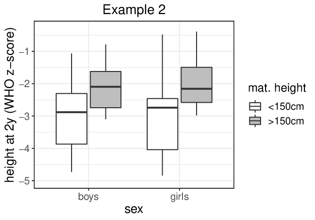
Example 2: We investigate the effect of the mother’s height (factor A) on the children’s height at the age of $2$ years. Both sexes (factor B) are included. We restrict to firstborns of unmarried mothers from the Philippines. For this analysis, we divide the women into the groups ”small” and ”tall” consisting of the women respectively being smaller and taller than the median height of $150$cm. The group ”small” consists of data for $n_{1}=8$ boys and $n_{2}=13$ girls, and in the group ”tall” there are data for $n_{3}=12$ boys and $n_{4}=11$ girls.

References

- Adiar (2007) L.S. Adiar. Size at birth and growth trajectories to young adulthood. American Journal of Human Biology, 19:327–337, 2007.
- Babu (1986) G.J. Babu. A note on bootstrapping the variance of sample quantile. Ann. Inst. Statist. Math., 38:439–443, 1986.
- Bahadur (1966) R.R. Bahadur. A note on quantiles in large samples. Ann. Math. Statist., 37:577–580, 1966.
- Baigent et al. (1998) C. Baigent, R. Collins, P. Appleby, S. Parish, P. Sleight, and R. Peto. ISIS-2: 10 year survival among patients with suspected acute myocardial infarction in randomised comparison of intravenous streptokinase, oral aspirin, both, or neither. BMJ, 316:1337, 1998.
- Bathke et al. (2009) A.C. Bathke, O. Schabenberger, R.D. Tobias, and L.V. Madden. Greenhouse-Geisser adjustment and the ANOVA-type statistic: cousins or twins? Amer. Statist., 63:239–246, 2009.
- Beyerlein (2014) A. Beyerlein. Quantile regression-opportunities and challenges from a user’s perspective. American Journal of Epidemiology, 180(3):330–331, 2014.
- Bhargava et al. (2009) S.K. Bhargava, H.S. Sachdev, C.H.D. Fall, C. Osmond, R. Lakshmy, D.J.P. Barker, S.K.D. Biswas, S. Ramji, D. Prabhakaran, and K.S. Reddy. Relation of serial changes in childhood body-mass index to impaired glucose tolerance in young adulthood. The New England Journal of Medicine, 250:865–875, 2009.
- Bonett (2006) D.G. Bonett. Confidence interval for a coefficient of quartile variation. Comput. Statist. Data Anal., 50:2953–2957, 2006.
- Brunner et al. (1997) E. Brunner, H. Dette, and A. Munk. Box-type approximations in nonparametric factorial designs. J. Amer. Statist. Assoc., 92:1494–1502, 1997.
- Cassidy et al. (2008) J. Cassidy, S. Clarke, E. Díaz-Rubio, W. Scheithauer, A. Figer, R. Wong, S. Koski, M. Lichinitser, T.-S. Yang, and F. Rivera. Randomized phase III study of capecitabine plus oxaliplatin compared with fluorouracil acid plus oxaliplatin as first-line therapy for metastatic colorectal cancer. Journal of Clinical Oncology, 26:2006–2012, 2008.
- Chung and Romano (2013) E.Y. Chung and J.P. Romano. Exact and asymptotically robust permutation tests. Ann. Statist., 41:484–507, 2013.
- de Onis et al. (2007) A. de Onis, A. Onyango, E. Borghi, A. Siyam, C. Nishida, and J. Siekmann. Develop,emt of a WHO growth reference for school-aged children and adolescents. Bull World Health Organ, 85:660–667, 2007.
- Efron (1979) B. Efron. Bootstrap methods: Another look at the jackknife. Ann. Statist., 7:1–26, 1979.
- Feng et al. (2011) X. Feng, X. He, and J. Hu. Wild bootstrap for quantile regression. Biometrika, 98(4):995–999, 2011.
- Fleming and Harrington (1991) T.R. Fleming and D.P. Harrington. Counting processes and survival analysis. Wiley Series in Probability and Mathematical Statistics: Applied Probability and Statistics. John Wiley & Sons, Inc., New York, 1991.
- Fried and Dehling (2011) R. Fried and H. Dehling. Robust nonparametric tests for the two-sample location problem. Stat. Methods Appl., 20:409–422, 2011.
- Friedrich et al. (2017a) S. Friedrich, E. Brunner, and M. Pauly. Permuting longitudinal data in spite of the dependencies. J. Multivariate Anal., 153:255–265, 2017a.
- Friedrich et al. (2017b) S. Friedrich, F. Konietschke, and M. Pauly. GFD: An R package for the analysis of general factorial designs. Journal of Statistical Software, 79:1–18, 2017b.
- Fung (1980) K.Y. Fung. Small sample behaviour of some nonparametric multi-sample location tests in the presence of dispersion differences. Stat. Neerl., 34:189–196, 1980.
- Ghosh et al. (1984) M. Ghosh, W.C. Parr, K. Singh, and G. J. Babu. A note on bootstrapping the sample median. Ann. Statist., 12:1130–1135, 1984.
- GISSI-2 (1990) The International Study Group GISSI-2. In-hospital mortality and clinical course of 20,891 patients with suspected acute myocardial infarction randomized between alteplase and streptokinase with or without heparin. Lancet, 336:71–75, 1990.
- Hall and Martin (1988) P. Hall and M.A. Martin. Exact convergence rate of bootstrap quantile variance estimator. Probab. Theory Related Fields, 80:261–268, 1988.
- Harrar et al. (2019) S.W. Harrar, F. Ronchi, and L. Salmaso. A comparison of recent nonparametric methods for testing effects in two-by-two factorial designs. J. Appl. Stat., 46:1649–1670, 2019.
- Hettmansperger and McKean (2010) T.P. Hettmansperger and J.W. McKean. Robust nonparametric statistical methods. Second edition. CRC Press, Boca Raton, FL, 2010.
- Hoeffding (1951) W. Hoeffding. A combinatorial central limit theorem. Ann. Math. Statistics, 22:558–566, 1951.
- Janssen (1997) A. Janssen. Studentized permutation tests for non-iid hypotheses and the generalized behrens-fisher problem. Statist. Probab. Lett., 36:9–21, 1997.
- Janssen and Pauls (2003) A. Janssen and T. Pauls. How do bootstrap and permutation tests work? Ann. Statist., 31:768–806, 2003.
- Johansen (1980) S. Johansen. The Welch-James approximation to the distribution of the residual sum of squares in a weighted linear regression. Biometrika, 67:85–92, 1980.
- Koenker and Hallock (2001) R. Koenker and K.F. Hallock. Quantile regression. Journal of Economic Perspectives, 15(4):143–156, 2001.
- Koenker and Machado (1999) Roger Koenker and Jose AF Machado. Goodness of fit and related inference processes for quantile regression. J. Amer. Statist. Assoc., 94(448):1296–1310, 1999.
- Koenker et al. (2019) Roger Koenker, Stephen Portnoy, Pin Tian Ng, Achim Zeileis, Philip Grosjean, and Brian D Ripley. Package ‘quantreg’: Quantile regression in R, 2019.
- Konietschke et al. (2015) F. Konietschke, A.C. Bathke, S.W. Harrar, and M. Pauly. Parametric and nonparametric bootstrap methods for general MANOVA. J. Multivariate Anal., 140:291–301, 2015.
- Kurz et al. (2015) A. Kurz, E. Fleischmann, D.I. Sessler, D.J. Buggy, C. Apfel, O. Akça, Factorial Trial Investigators, E. Fleischmann, E. Erdik, and K. Eredics. Effects of supplemental oxygen and dexamethasone on surgical site infection: a factorial randomized trial. British Journal of Anaesthesia, 115:434–443, 2015.
- Lubsen and Pocock (1994) J. Lubsen and S.J. Pocock. Factorial trials in cardiology: pros and cons. European Heart Journal, 15:585–588, 1994.
- McKean and Schrader (1984) J.W. McKean and R.G. Schrader. A comparision of methods for studentizing the sample mean. Commun. Statist. B, 13:751–773, 1984.
- Mehta et al. (2010) S.R. Mehta, J.-F. Tanguay, J.W. Eikelboom, S.S. Jolly, C.D. Joyner, C.B. Granger, D.P. Faxon, H.-J. Rupprecht, A. Budaj, and A. Avezum. Double-dose versus standard-dose clopidogrel and high-dose versus low-dose aspirin in individuals undergoing percutaneous coronary intervention for acute coronary syndromes (CURRENT-OASIS 7): a randomised factorial trial. Lancet, 376(9748):1233–1243, 2010.
- Nadaraya (1965) E.A. Nadaraya. On non-parametric estimates of density functions and regression curves. Theory Probab. Appl., 10:186–190, 1965.
- Neuhaus (1993) G. Neuhaus. Conditional rank tests for the two-sample problem under random censorship. Ann. Statist., 21:1760–1779, 1993.
- Pauly (2011) M. Pauly. Discussion about the quality of f-ratio resampling tests for comparing variances. TEST, 20:163–179, 2011.
- Pauly et al. (2015) M. Pauly, E. Brunner, and F. Konietschke. Asymptotic permutation tests in general factorial designs. J. R. Stat. Soc. Ser. B. Stat. Methodol., 77:461–473, 2015.
- Potthoff (1963) R.F. Potthoff. Use of the wilcoxon statistic for a generalized behrens-fisher problem. Ann. Math. Statist., 34:1596–1599, 1963.
- Price and Bonett (2001) R.M. Price and D.G. Bonett. Estimating the variance of the sample median. J. Stat. Comput. Simul, 68:295–305, 2001.
- R Core Team (2019) R Core Team. R: A language and environment for statistical computing. R Foundation for Statistical Computing, Vienna, Austria, 2019. URL http://www.R-project.org.
- Rao and Mitra (1971) C.R. Rao and S.K. Mitra. Generalized inverse of matrices and its applications. John Wiley & Sons, Inc., New York-London-Sydney, 1971.
- Richter et al. (2007) L.M. Richter, J.M. Norris, S.A. anc Pettifor, D. Yach, and N. Cameron. Cohort profile: Mandela’s children: the 1990 birth to twenty study in south africa. International Journal of Epidemiology, 36:504–511, 2007.
- Richter et al. (2012) L.M. Richter, C.G. Victora, P.C. Hallal, L.S. Adair, S.K. Bhargava, C.H. Fall, N. Lee, R. Martorell, S.A. Norris, H.S. Sachdev, A.D. Stein, and COHORTS Group. Cohort profile: the consortium of health-orientated research in transitioning societies. International Journal of Epidemiology, 43:621–626, 2012.
- Schuster (1969) E.F. Schuster. Estimation of a probability density function and its derivatives. Ann. Math. Statist., 40:1187–1195, 1969.
- Sen (1962) P.K. Sen. On studentized non-parametric multi-sample location tests. Ann. Inst. Statist. Math., 14:119–131, 1962.
- Serfling (2009) R.J. Serfling. Approximation theorems of mathematical statistics. John Wiley & Sons, New York, NY, 2009.
- Shorack and Wellner (2009) G.R. Shorack and J.A. Wellner. Empirical processes with applications to statistics. Society for Industrial and Applied Mathematics (SIAM), Philadelphia, PA, 2009.
- Silverman (1978) B.W. Silverman. Weak and strong uniform consistency of the kernel estimate of a density and its derivatives. Ann. Statist., 6:177–184, 1978.
- Silverman (1986) B.W. Silverman. Density Estimation. Chapman and Hall, London, 1986.
- Smaga (2017) Ł. Smaga. Diagonal and unscaled wald-type tests in general factorial designs. Electron. J. Stat., 11:2613–2646, 2017.
- Stein et al. (2008) A.D. Stein, P. Melgar, J. Hoddinott, and R. Martorell. Cohort profile: the Institute of Nutrition of Central America and Panama (INCAP) nutrition trial cohort study. International Journal of Epidemiology, 37:716–720, 2008.
- Umlauft et al. (2017) M. Umlauft, F. Konietschke, and M. Pauly. Rank-based permutation approaches for non-parametric factorial designs. British Journal of Mathematical and Statistical Psychology, 70:368–390, 2017.
- van der Vaart and Wellner (1996) A.W. van der Vaart and J.A. Wellner. Weak convergence and empirical processes. Springer Series in Statistics. Springer-Verlag, New York, 1996.
- van der Vaart and Wellner (2000) A.W. van der Vaart and J.A Wellner. Preservation theorems for Glivenko-Cantelli and uniform Glivenko-Cantelli classes. In High dimensional probability II, pages 115–133. Springer, 2000.
- Victora and Barros (2006) C.G. Victora and F.C. Barros. Cohort profile: the 1982 Pelotas (Brazil) birth cohort study. International Journal of Epidemiology, 35:237–242, 2006.
- WHO Multicentre Growth Reference Study Group (2006) WHO Multicentre Growth Reference Study Group. WHO child growth standards based on length/height, weight and age. Acta Paediatr Suppl, 450:76 – 85, 2006.
- Zhang (2012) J.-T. Zhang. An approximate degrees of freedom test for heteroscedastic two-way ANOVA. J. Statist. Plann. Inference, 142:336–346, 2012.