Achieving the ultimate precision limit in quantum NMR spectroscopy
Abstract
The ultimate precision limit in estimating the Larmor frequency of unentangled rotating spins is well established, and is highly important for magnetometers, gyroscopes and many other sensors. However this limit assumes perfect, single addressing, measurements of the spins. This requirement is not practical in NMR spectroscopy, as well as other physical systems, where a weakly interacting external probe is used as a measurement device. Here we show that in the framework of quantum nano-NMR spectroscopy, in which these limitations are inherent, the ultimate precision limit is still achievable using control and a finely tuned measurement.
I INTRODUCTION
Nuclear Magnetic Resonance (NMR) spectroscopy is a revolutionary field that has had a considerable impact on science and medicine alike. It enables chemists to deduce molecular proprieties, and is best known for magnetic resonance imaging. The main idea behind the technology is that applying a large external magnetic field creates a macroscopic magnetization of the test sample. When a resonance pulse is implemented, the magnetization vector is transferred into the transverse plane, where it precesses around the external magnetic field axis. The oscillatory magnetic field of the sample can be sensed classically, and its spectral decomposition carries the target informationAbragam 1961; Slichter 1963; Filler 2009; Rinck 2019; Ginsberg 2011.
Nano-scale NMR is a recent extension of this idea, that focuses on the measurement of the NMR spectra of minute samples. The main challenge stems from the fact that the net polarization of these samples cannot be detected using macroscopic devices. While various directions are being pursued to confront this challenge, one of the most promising is the Nitrogen-Vacancy (NV) based spectrometer which relies on a quantum emitter as a nano scale detector. The NV center is a natural candidate, since in the past decade it has been shown to be an excellent magnetometer on the nano-scale Doherty et al. 2013; Jensen et al. 2017, and many successful experiments have been carried out in platform similar to fig. 1 Staudacher et al. 2013; DeVience et al. 2015; Mamin et al. 2013; Shagieva et al. 2018; Pfender et al. 2019; Aslam et al. 2017; Glenn et al. 2018a. To date, most ensemble experiments in the field have been conducted with bulk NVs, since surface effects and finite polarization limit the sensitivity attained by the shallow ones. These experiments were able to measure impressively narrow spectraGlenn et al. 2018a. However, since the effective sample volume scales with the NV’s depth, the use of shallow NVs is inevitable if one aims to interrogate ultra-small samples.
Whether the sensing is quantum or classic, the acquired signal is
| (1) |
where is the number of nuclei in the ensemble, is their Larmor frequency and is the signal amplitude generated by a single nucleus. In the quantum case is replaced by , the phase acquired from a single nucleus, which is a function of the interaction strength and the interrogation time. The uncertainty of the frequency measurement of the signal (1) scales inversely with the derivative and thus can be written as
| (2) |
where the first equality is correct for either classic or quantum sensing with some constant , while the second is correct only for the quantum case. We know, however, that in a noisy environment the optimal precision, achievable by performing Ramsey spectroscopy on each nucleus Braunstein and Caves 1994; Huelga et al. 1997 is
| (3) |
Comparing Eqs. (2) and (3) yields the restriction . Since the phase is a function of the interaction between the sensor and the nuclei, which increases as the sensor is brought into close proximity with the sample, the behavior of the signal must change when . Therefore, there is a critical depth , for which the behavior of the signal transforms from classical to quantum (see the right side of Fig. 1). For common parameters of liquids, an interrogation time of and a fully polarized nuclear spin ensemble, we find that (see section 3 for details). For finite polarization, , the critical distance changes , such that for it drops to for the same . We henceforth refer to Eq. (2) as ”Heisenberg scaling with ” or as the ”weak limit” for reasons that will readily become apparent, and to Eq. (3) as the Ramsey limit or the standard quantum limit (SQL).
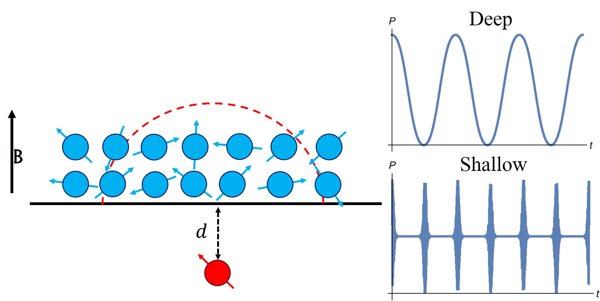
Here we provide and analyze a nano-NMR protocol and show that for an NV with a given depth, for short measurement times, our protocol achieves a ”Heisenberg-like” scaling with N, which is greatly reduced by the weak NV-nucleus coupling, whereas for long measurement times, the scaling changes to the SQL with respect to N and does not depend on the coupling. Moreover, we show that using an adaptive measurement method, for long measurement times, the uncertainty scales effectively, up to a prefactor, as the fundamental Ramsey limit that requires individual addressing of each nucleus. Alternatively, for a given measurement time, the precision of the protocol changes from the weak limit to the SQL for increasingly shallow NVs. In other words, even when using shallow NVs for probing an ensemble with finite polarization in the weak coupling limit - where the NV-nucleus coupling constant multiplied by the measurement time is much smaller than - our protocol achieves an accuracy scaling that does not strictly depend on the coherence time of the NV or the NV-nucleus coupling constant and follows the SQL with respect to N.
The paper is organized as follows. We start with a simplified model for nano-NMR to introduce our protocol and the main results. Then we explain how this model can be adapted to include more realistic settings and we modify our results accordingly. Finally, we discuss possible modifications to the protocol and provide an overview of the work.
II results
II.1 Simplified Model: Constant Coupling
Let us start with a simplified model that captures the essentials. The physical system consists of a quantum sensor, taken to be a two level system with energy gap , and an ensemble of spin-1/2 nuclei with energy gap as described by the Hamiltonian
| (4) |
where is the Pauli matrix of the sensor/j-th nucleus in the direction. The NV and the nuclei interact with a constant coupling
| (5) |
Our protocol for the estimation of starts by initializing the system to the state and the interaction is suppressed. Note, that we explicitly assume that the nuclear spins are completely polarized in the direction. The propagation in the interaction picture with respect to the sensor’s energy gap is
| (6) |
Then is turned on while is turned off, so the propagation by an additional time will result in
| (7) |
where . The reduced density matrix of the sensor after both steps is
| (8) |
where the off diagonal element is given by
| (9) |

To obtain the product it is convenient to write the complex number (9) in a polar representation
| (10) | ||||
| (11) |
where the approximations are made using the assumption of weak coupling, . We henceforth refer to the accumulated phase, , as ”the signal” since it corresponds to the ”classical” signal (1) with the aforementioned accumulated phase , and we refer to as the decay. The decay is caused by the entanglement between the NV and nuclear spin ensemble, as illustrated in fig. 2. For times the dynamics is purely classical because the rotation around the axis is trivial, whereas for other times the rotation causes the sensor state to be entangled with the collective state of the ensemble. Therefore, the dimensionless quantity characterizing the decay, , is interpreted as the back-action. Because the coupling constant depends on the distance between the sensor and the sample, the transition from weak to strong back-action is dictated by the NV’s depth for a given . This transition is the one predicted in the introduction, as it occurs when . Substituting Eqs. (10) and (11) into (9),
| (12) |
The measurable quantity associated with (12) is the probability distribution,
| (13) |
which is related to eq. (12) by . The function (13) is the non-approximate form of (1). It is drawn on the right hand side of Fig. 1 with and (top) or (bottom) which correspond to weak and strong back-action respectively.
In order to determine the precision of the estimation of we use the tools of quantum metrology. The Fisher Information for the discrete probability dependent on a parameter g is defined as DeGroot and Schervish 2012. For a quantum system one can optimize over all possible measurement bases. This leads to the definition of Quantum Fisher Information (QFI) Degen et al. 2017. For a density matrix , the QFI about is given by Braunstein and Caves 1994. The precision of any measurement is bounded by the Cramer-Rao bound, . Since this is a tight bound, we use it henceforth to quantify precision. For the density matrix (8) the QFI can be expressed as the relevant Bures distance Slater 1998; Braunstein and Caves 1994:
| (14) |
thus, eqs. (10), (11) and (14) lead to
| (15) |
where . In the limit of weak back-action, ,
| (16) | ||||
| (17) |
The QFI in this limit is optimal when
| (18) |
since the derivative of the signal is then maximal and the decay is negligible. For the optimal time (18), the QFI (15) is
| (19) |
which corresponds to the uncertainty as in (2) with . Thus, in the limit of weak back-action, we achieve an uncertainty that scales as in exchange for the large factor .
Achieving better precision, however, requires , where consequently, the decay starts to affect the quantum sensor. The optimal time (18), therefore, must change to account for the decay. The new time is approximately
| (20) |
for which the QFI (15) is
| (21) |
and corresponds to the uncertainty The decay, therefore, ”corrects” the apparent Heisenberg scaling for high precision. This is a surprising result, as the uncertainty is limited solely by the coherence time of the nuclei as in Schmitt et al. 2017; Pfender et al. 2019; Boss et al. 2017; Glenn et al. 2018b; Bucher et al. 2018; Gefen et al. 2018 and it does not depend on the coupling constant . Moreover, if we could manipulate and read-out each nucleus individually, the optimal QFI would be attained by the Ramsey limit (3). Therefore, up to the numerical factor of our protocol is the optimal one. Figure 3 compares the different QFI scalings to our protocol.
To obtain this QFI we assume optimization of and the measurement basis, which requires knowledge of . As shown in fig. 4, the QFI increases with , but it also becomes increasingly narrow, such that a more accurate estimation of is required to achieve it. This, however, can be resolved by using an adaptive measurement protocol - first a non-optimal measurement is performed to acquire an estimate of , and the next measurement’s duration is optimized according to the previous measurement’s outcome. This can be repeated until the optimal precision is attained. An analysis of this model using multiple sensors can be found in Sup.
II.2 Spatially dependent coupling
In the previous section we presented the simplified model with the interaction Hamiltonian (5). This is an approximate form of the dipole-dipole interaction Hamiltonian, which can be written as
| (22) |
In the interaction picture with respect to sensor’s energy gap, after taking the rotating wave approximation, the remaining terms are
| (23) |
If we further assume that the nuclei can be driven in the direction sufficiently fast compared to the interaction and the entanglement generation rate, we arrive at the Hamiltonian
| (24) |
The difference between (24) and the toy model (5) is that the coupling differs from one nucleus to the other. It depends, in fact, on the position of the nucleus and, therefore, also on time. Further description of the interaction requires specific realization of the sensor, henceforth we use the NV center. In a spherical coordinate system, where the NV is found at the origin, the NV’s magnetization axis coincides with the axis and the nucleus position is denoted by , the coefficients are given by
| (25) |
with the physical coupling constant , where is the vacuum permeability, is the reduced Plank constant and are the electronic/nuclear gyro-magnetic ratios.
Repeating the derivation of the previous section with the interaction (24), eq. (9) becomes
| (26) |
where . In the limit of weak coupling, , (26) can be approximated to
| (27) |
There is therefore a dependence only on and the QFI reads,
| (28) |
The quantity that determines the behavior of the optimal QFI is :
| (29) |
The regime of interest is , where, as we readily show, a modified SQL scaling can be achieved. Note that where equality is attained only for homogeneous couplings.
To obtain the QFI in a nano-NMR scenario, we need therefore to find the relevant . The results will of course depend on the parameters of the problem. We denote by the nuclei number density, the diffusion coefficient of the sample, the depth of the NV and the NV’s tilting angle, measured between the normal to the diamond surface and it’s magnetization axis. Let us first calculate assuming ,
| (30) |
While is proportional to the average magnetic field, it can be observed that goes as the magnetic field auto-correlation,
| (31) | ||||
where is an average over realizations and is the stationary diffusion propagator from to with time difference . The correlation decays with a characteristic time of , which dictates the behavior of Although the full expression of is involved Cohen et al. 2019, the asymptotic behavior is rather simple,
| (32) |
where is the instantaneous fluctuation in the magnetic field:
| (33) | ||||
The mean field, (30), and , (33), can be estimated more explicitly,
| (34) | ||||
| (35) |
where we took and as the water number density. We use these quantities for the remainder of the article in our quantitative estimates.
The validity condition of the second order approximation in can be put into physical terms with the definitions (30) and (33) ; e.g. Eqs. (27) and (28) are valid when , which means that the polarization should be larger than the statistic polarization. Hence, for increasingly shallow NVs, higher orders should be taken into account (see discussion in Sup).
We are now fully equipped to calculate the optimal QFI by substituting and (Eqs. (30) and (32) respectively) into (29). In the weak back-action regime, , the optimal QFI reads:
| (36) |
For strong back-action the optimal QFI depends explicitly on ,
| (37) |
where the optimal is given by
| (38) |
Note that the transition from (36) to (37) occurs when , which defines the critical depth in terms of the physical parameters.
The result (36) and the short times limit of (37) are similar to those of the simplified model, with the difference that due to the dipolar interaction and the geometry, there is an additional dependence on the NV’s tilting angle. In (37) this is translated into a change in the total number of particles in (21) by an effective number , which is proportional to the number of particles in the effective interaction region.
The long times regime of Eq. (37) may look puzzling since for large enough we can get an arbitrarily large QFI, which seems paradoxical. This arbitrarily large QFI is due to the fact that we consider an infinite sample volume; i.e. an infinite amount of nuclear spins. Restricting ourselves to a finite volume, , with nuclei yields the restriction by imposing the SQL. This limitation on can be taken to be Sup, where is the volumetric diffusion time; i.e., the characteristic time it takes for a particle to move from one of the volume’s boundaries to another. For sufficiently long times, , the QFI scaling changes to
| (39) |
This is the equivalent of (21). In the simplified model the sensor is coupled equally to all the nuclei from the start; therefore, the QFI scales with the total number of nuclei, while in reality the dipolar interaction creates an effective cut off, such that in short times the QFI scales as and only after a long time, , when all the nuclei have passed through the interaction region, does the QFI scale with the total number of nuclei. As in Eq. (21), in this model the QFI is not limited by the coherence time of the NV, , but only by the coherence time of the nuclei which is usually longer by orders of magnitude.
II.3 Undriven nuclei
In the previous section we assumed that we can drive the nuclei sufficiently fast to achieve the approximate dynamics given by (24). In some experimental settings this is unfeasible for practical reasons. Hence, in what follows, we drop this assumption. The approximate dipolar Hamiltonian (23) is rewritten as
| (40) |
The NV is then driven with pulses every time so that the effective pulse frequency is close to . This yields the effective Hamiltonian Sup
| (41) |
and the remaining free Hamiltonian
| (42) |
where and . Following the same protocol as before Sup the signal is
| (43) |
where the average magnetic field is as in the driven case, (30). The decay, however, changes to
| (44) |
for times , where
| (45) | ||||
| (46) |
are the quantum and classical contributions to the instantaneous fluctuation of the magnetic field and is given by (33).
Comparing Eqs. (43) and (44) to the results of the previous section (30) and (32), note that the signal is the same upto a prefactor of order and a constant known phase. The decay, however changes, so it is non-zero for any given time . This is expected, since previously the interaction caused all the nuclei to rotate around the same axis, which resulted in an entanglement induced decay. Without the external drive, the interaction causes each nuclear spin to rotate around a different axis in the xy plane of the Bloch sphere, which induces additional classical dephasing (see supplementary fig. S2). It is worth pointing out that the quantum contribution (45) can be negative, but the total is always real and positive. When the decay is small, , we retrieve the result (36) up to a prefactor , since it only depends on the signal.
If the decay is dominant, the classical and quantum decay compete when optimizing the QFI. On the one hand the strong back-action regime requires , which implies that has to be large enough. On the other hand, the classical dephasing causes an exponential decrease in the QFI, , that depends only on . To limit this effect we require . Hence, when the nuclei are undriven fine tuning of is required in order to optimize these competing processes. The optimal protocol will no longer be universal and will depend on the physical parameters.
First, we assume strong back-action, in order to derive the analog protocol to the previous sections, and to emphasis our last statement regarding the decay. The optimal satisfies
| (47) |
for which the QFI is
| (48) |
As aforementioned, the QFI, (48), has a reduction by an exponential factor compared to the previous result (37), arising from the classical dephasing. As long as we can satisfy the strong back-action requirement, while limiting the classical decay by taking . This results in a reduction by a reasonable factor of . This inequality is a function of the NV’s tilting angle alone, and is correct for . Since the NV’s natural tilting angle is this is approximately the case, where the slight deviation will lead to further reduction of the QFI by a small factor. Another issue with this strategy is that it is not guaranteed that , and indeed for a typical number density and an NV depth of , the time required is .
Obtaining other scalings is possible by optimizing and , depending on the parameters; for example, by choosing we achieve
| (49) |
which is the same result as in (37). Note that this is the case of ”critical back-action”, when , therefore smaller will lead to the weak back-action limit and larger will cause an exponential decrease. Since the same typical parameters yield , the lack of external drive reduces Eq. (37) by a factor of . The results for can be derived by using reasoning similar to the previous section. However, the long times limit of (37) and (39) will typically no longer be achievable because the optimal will be much longer than .
II.4 Finite polarization
We now consider the more general case, where the spin’s polarization is finite. We assume that the spins are statistically polarized, such that the initial density matrix of the system is
| (50) |
For the interaction Hamiltonian (24), following our protocol, the individual spin’s signal and decay (in the limit ) are
| (51) | ||||
| (52) |
where and are given by (30) and (33). The signal, therefore is the same as the one of a fully polarized ensemble, (30) with , where we denote the polarization by . The decay, on the other hand, consists of two terms: one that can be associated with the polarized dynamics and the other with the unpolarized dynamics. The former, is the same term as the in the fully polarized case (32), multiplied by the polarization squared, . The latter is the constant term which is proportional to the Bernoulli variance and stems from classical dephasing. For a small decay the QFI will then be
| (53) |
while for a large decay, as in the previous section, an optimization over and is required according to the physical parameters. The two possibilities presented in the last section translate here to
| (54) | ||||
| (55) |
which yield
| (56) | ||||
| (57) |
respectively.
III Conclusion
We provide a protocol for nano-NMR that achieves the SQL up to a prefactor in the strong back-action regime. Moreover, the uncertainty does not depend on the coherence time of the sensor or the probe-nuclear coupling. Our analysis shows that the full SQL, with respect to the number of nuclei, requires a fully polarized sample, an ability to manipulate the nucleus-sensor interaction via a sufficient external drive, and interrogation times longer than the characteristic volumetric diffusion time. Deviation from these standards results in a reduced effective number of particles, which is a function of the aforementioned parameters and the NV’s tilting angle. These difficulties, however, can be mitigated by using multiple sensors. These features make it highly applicable for sensing very small samples, which is the ultimate goal of the field.
Acknowledgments
A. R. acknowledges the support of ERC grant QRES, project No. 770929, grant agreement No 667192(Hyperdiamond), and the ASTERIQS and DiaPol projects.
References
- Abragam (1961) A. Abragam, The Principles of Nuclear Magnetism (Oxford U.P., Oxford, 1961) Chap. VIII.
- Slichter (1963) C. P. Slichter, Principles of Magnetic Resonance (Springer-Verlag Berlin Heidelberg, New York, 1963).
- Filler (2009) A. Filler, Nature Precedings (2009), 10.1038/npre.2009.3267.3.
- Rinck (2019) P. A. Rinck, Magnetic Resonance in Medicine (BoD, Germany, 2019) Chap. 19.
- Ginsberg (2011) J. Ginsberg, “Nmr and mri: Applications in chemistry and medicine,” (2011).
- Doherty et al. (2013) M. W. Doherty, N. B.Manson, P. Delaney, F. Jelezko, J. Wrachtrup, and L. C. L. Hollenberg, Phys. Rep. 528, 1 (2013).
- Jensen et al. (2017) K. Jensen, P. Kehayias, and D. Budker, “Magnetometry with nitrogen-vacancy centers in diamond,” in High Sensitivity Magnetometers, edited by A. Grosz, M. Haji-Sheikh, and S. Mukhopadhyay (Springer, Cham, Berlin, Heidelberg, 2017).
- Staudacher et al. (2013) T. Staudacher, F. Shi, S. Pezzagna, J. Meijer, J. Du, C. A. Meriles, F. Reinhard, and J. Wrachtrup, SCIENCE 339, 6119 (2013).
- DeVience et al. (2015) S. J. DeVience, L. M. Pham, I. Lovchinsky, A. O. Sushkov, N. Bar-Gill, C. Belthangady, F. Casola, M. Corbett, H. Zhang, M. Lukin, H. Park, A. Yacoby, and R. L. Walsworth, Nat. Nanotech 10, 129 (2015).
- Mamin et al. (2013) H. J. Mamin, M. Kim, M. H. Sherwood, C. T. Rettner, K. Ohno, D. D. Awschalom, and D. Rugar, SCIENCE 339 (2013), 10.1126/science.1231540.
- Shagieva et al. (2018) F. Shagieva, S. Zaiser, P. Neumann, D. B. R. Dasari, R. Stöhr, A. Denisenko, R. Reuter, C. A. Meriles, and J. Wrachtrup, Nano Lett. 18, 3731 (2018).
- Pfender et al. (2019) M. Pfender, P. Wang, H. Sumiya, S. Onoda, W. Yang, D. B. R. Dasari, P. Neumann, X.-Y. Pan, J. Isoya, R.-B. Liu, and J. Wrachtrup, Nat. Commun 10, 594 (2019).
- Aslam et al. (2017) N. Aslam, M. Pfender, P. Neumann, R. Reuter, A. Zappe, F. F. de Oliveira, A. Denisenko, H. Sumiya, S. Onoda, J. Isoya, and J. Wrachtrup, SCIENCE 357 (2017), 10.1126/science.aam8697.
- Glenn et al. (2018a) D. R. Glenn, D. B. Bucher, J. Lee, M. D. Lukin, H. Park, and R. L. Walsworth, Nature 555, 351 (2018a).
- Braunstein and Caves (1994) S. L. Braunstein and C. M. Caves, Phys. Rev. Lett. 72, 3439 (1994).
- Huelga et al. (1997) S. F. Huelga, C. Macchiavello, T. Pellizzari, A. K. Ekert, M. B. Plenio, and J. I. Cirac, Phys. Rev. Lett. 79, 3865 (1997).
- DeGroot and Schervish (2012) M. H. DeGroot and M. J. Schervish, Probability and statistics (Pearson Education, 2012).
- Degen et al. (2017) C. L. Degen, F. Reinhard, and P. Cappellaro, Reviews of modern physics 89, 035002 (2017).
- Slater (1998) P. B. Slater, Physics Letters A 244, 35 (1998).
- Schmitt et al. (2017) S. Schmitt, T. Gefen, F. M. Stürner, T. Unden, G. Wolff, C. Müller, J. Scheuer, B. Naydenov, M. Markham, S. Pezzagna, J. Meijer, I. Schwarz, M. Plenio, A. Retzker, L. P. McGuinness, and F. Jelezko, SCIENCE 356, 6340 (2017).
- Boss et al. (2017) J. Boss, K. Cujia, J. Zopes, and C. Degen, Science 356, 837 (2017).
- Glenn et al. (2018b) D. R. Glenn, D. B. Bucher, J. Lee, M. D. Lukin, H. Park, and R. L. Walsworth, Nature 555, 351 (2018b).
- Bucher et al. (2018) D. B. Bucher, D. R. Glenn, H. Park, M. D. Lukin, and R. L. Walsworth, arXiv preprint arXiv:1810.02408 (2018).
- Gefen et al. (2018) T. Gefen, M. Khodas, L. P. McGuinness, F. Jelezko, and A. Retzker, Physical Review A 98, 013844 (2018).
- (25) “See supporting information,” .
- Cohen et al. (2019) D. Cohen, R. Nigmatullin, O. Kenneth, F. Jelezko, M. Khodas, and A. Retzker, arXiv preprint arXiv:1903.02348 (2019).