Algebraic multigrid methods for saddle point systems arising from mortar contact formulations

We consider two solid bodies, which are represented by $\Omega_{0}^{(1)}$, $\Omega_{0}^{(2)}\subset\mathbb{R}^{d}$ with $d\in\{2,3\}$ in the reference configuration. Their surfaces $\partial\Omega_{0}^{{(i)}}$, $i\in\left\{1,2\right\}$ are decomposed into three disjoint subsets $\Gamma_{{\mathsf{D}}}^{{(i)}}$, $\Gamma_{{\mathsf{N}}}^{{(i)}}$ and $\Gamma_{{\mathsf{c}}}^{{(i)}}$ denoting the Dirichlet boundary, the Neumann boundary, and the potential contact interface with unknown contact tractions $\boldsymbol{t}_{{\mathsf{c}}}^{(i)}$, respectively. The solid bodies themselves are governed by nonlinear elasticity. Since we are only interested in the algebraic block structure of the final system of equations after discretization and linearization, it is sufficient to discuss a quasi-static contact problem with only two deformable bodies.

In order to describe the contact phenomenon, we state the Hertz-Signorini-Moreau conditions

Therein, $g_{\mathrm{n}}$ defines a so-called gap function, which measures the distance of a point on the slave interface $\gamma_{{\mathsf{c}}}^{(\mathcal{S})}$ to the projected corresponding point on the master side $\gamma_{{\mathsf{c}}}^{(\mathcal{M})}$ of the contact interface in the current configuration. Furthermore, $p_{\mathrm{n}}$ denotes the normal contact traction. In the mathematical formulation, one introduces the negative slave side contact traction $\boldsymbol{t}_{{\mathsf{c}}}^{(1)}$ as Lagrange multiplier, i.e., $\boldsymbol{\lambda}=-\boldsymbol{t}_{{\mathsf{c}}}^{(1)}$. Using $\boldsymbol{n}$ to denote the outward unit normal vector, the normal part of the contact stress can be denoted by $\lambda_{\mathrm{n}}:=\boldsymbol{\lambda}^{\mathsf{T}}\boldsymbol{n}$ and the tangential part by $\boldsymbol{\lambda}_{\mathrm{\tau}}:=\boldsymbol{\lambda}-\lambda_{\mathrm{n}}\boldsymbol{n}$.

We employ the usual function spaces $\boldsymbol{\mathcal{U}}^{(i)}$ and $\boldsymbol{\mathcal{V}}^{(i)}$ for the displacement field $\boldsymbol{u}$ of the the solid body and its weighting function $\boldsymbol{v}$, respectively. Furthermore, a suitable function space $\boldsymbol{\mathcal{M}}_{+}$ for the Lagrange multiplier field $\boldsymbol{\lambda}$ and its weighting function $\boldsymbol{\mu}$ is assumed. The weak form of the governing equations then reads: Find $\bigl(\boldsymbol{u},\boldsymbol{\lambda}\bigr)\in\boldsymbol{\mathcal{U}}\times\boldsymbol{\mathcal{M}}_{+}$ such that

Herein, the internal and external virtual work contributions $\delta\mathcal{W}_{\mathrm{int,ext}}$ are defined as usual in nonlinear solid mechanics (cf. [96] for example) and, thus, further details are omitted. The second term in (2a) can be identified as contact virtual work $\delta\mathcal{W}_{{\mathsf{c}}}$ and the expression in (2b) as variational inequality formulation of the contact constraints. An extension to frictional contact based on Coulomb’s law is straightforward and can be found in our previous work [28] for example.

For spatial discretization of the displacement field, either isoparametric finite elements with first-order and second-order Lagrange interpolation or isogeometric analysis (IGA) with NURBS-based shape functions are employed. After discretization, the discrete representation of displacement unkowns is given by the nodal degrees of freedom (DOFs)

Therein, the $\boldsymbol{u}_{\mathcal{N}_{i}}$, $i\in\{1,2\},$ contain all degrees of freedom associated with the mesh nodes of the corresponding solid body without the nodes at the contact interface, where we use the convention that indices $1$ and $2$ denote the slave and master “body”, respectively. The degrees of freedom associated with the contact interface on the slave and master side are represented by $\boldsymbol{u}_{\mathcal{S}}$ and $\boldsymbol{u}_{\mathcal{M}}$, respectively.

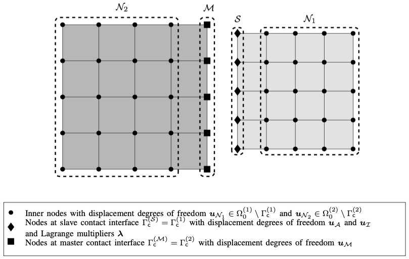
Since (2) represents a mixed variational form, we also have to discretize the Lagrange multiplier field $\boldsymbol{\lambda}$. We choose to follow a mortar approach for its mathematical properties and its superiority to other schemes [21, 59, 60, 89, 93]. As usual for mortar methods, the Lagrange multiplier field is discretized on the slave side contact interface $\gamma_{{\mathsf{c}}}^{(\mathcal{S})}$ in the current configuration. We either use standard ansatz functions, i.e. Lagrange polynomials with a trace space relation with the underlying volume element, or dual shape functions. The latter satisfy a biorthogonality property and, thus, allow for a computationally cheap condensation of the additional unknown Lagrange multipliers from the final system of equations. For details on dual basis functions in the context of mortar-based contact discretizations, we refer to [55, 88, 42]. Their interplay with preconditioners for iterative linear solvers has been discussed in our previous work [85]. The vector of discrete Lagrange multipliers is now referred to as $\boldsymbol{\lambda}$. A schematic mesh illustrating interior, slave interface, and master interface nodes is sketched in Figure 1.

The final spatially discretized formulation of the quasi-static frictionless problem (2) using the nodal vector representation now emerges as

The internal forces ${\boldsymbol{\mathsf{f}}}_{\textnormal{int}}(\boldsymbol{u})$ and external forces ${\boldsymbol{\mathsf{f}}}_{\textnormal{ext}}$ are common in nonlinear finite element methods and need no further explanation. The discrete vector of contact forces ${\boldsymbol{\mathsf{f}}}_{\textnormal{co}}$ is computed based on two mortar matrices $\mathsf{D}$ and $\mathsf{M}$, arising from the integral over the slave interface $\gamma_{{\mathsf{c}}}^{(\mathcal{S})}$ in (2a), and the discrete Lagrange multiplier vector $\boldsymbol{\lambda}$. For details regarding the computation of $\mathsf{D}$ and $\mathsf{M}$, see [54, 59] for example. Using $\bigl(\widetilde{g}_{\mathrm{n},\mathrm{h}}\bigr)_{j}$ to denote the discrete weighted gap function at node $j$, a closer look at the discrete contact constraints reveals that (3b) basically represents a discrete version of the Karush–Kuhn–Tucker (KKT) type conditions in (1) with an additional weighting based on the Lagrange multiplier shape functions $\psi_{j}$, while the nodal enforcement of frictionless sliding in (3c) is straightforward anyway.

Since the discrete contact constraints summarized in (3b) are still formulated as inequalities, an active set strategy usually referred to as primal-dual active set strategy (PDASS) is needed in addition to the usual nonlinear solution procedure to identify the currently active and inactive contact regions $\mathcal{A}$ and $\mathcal{I}=\mathcal{S}\setminus\mathcal{A}$, respectively. It has been demonstrated in [17, 35, 61] that the PDASS can equivalently be interpreted as a semi-smooth Newton method, thus allowing for an integrated treatment of all nonlinearities (including the search for the active set) within one single Newton–Raphson type iteration loop. Meanwhile, many successful applications to small and large deformation contact problems can be found in the literature [28, 37, 36, 54].

For efficient iterative solution strategies based on multigrid methods for nonlinear contact problems, one is primarily interested in the structure of the linear systems arising in each nonlinear iteration step of the underlying Newton–Raphson scheme. For the sake of brevity, details on the linearization process and on the Newton–Raphson procedure are omitted here and the interested reader is instead referred to [57, 54].

Consistent linearization of (3) and a subsequent update of the active set $\mathcal{A}$ and inactive set $\mathcal{I}$ yields the system

to be solved in every nonlinear iteration. The $2\times 2$ block matrix indicated by the dashed lines in (4) describes a linear system with a typical generalized saddle point structure. The upper left block consists of the entries of the tangential stiffness matrix (i.e. linearized internal forces) as well as linearizations of contact forces w.r.t. displacement degrees of freedom $\boldsymbol{u}$. The upper right block mirrors the discrete contact operator ${\boldsymbol{\mathsf{C}}}(\boldsymbol{u})$, i.e. basically the two mortar matrices $\mathsf{D}$ and  $\mathsf{M}$, representing the linearizations of the contact forces w.r.t. the Lagrange multiplier unknowns $\lambda$. The kinematic constraints are incorporated in the bottom left block. The very simple sixth block row emerges from (3b) and (3c) for inactive nodes, while the last block row imposes frictionless sliding in the directions tangential to the contact interface.

The distinct pattern of zero entries in the upper left block reveals that the two solid bodies (indices $\mathcal{N}_{1}$ and $\mathcal{N}_{2}$) are indeed only coupled through the slave and master sides of the contact interface (indices $\mathcal{S}$ and $\mathcal{M}$). Even though formulated for two solid bodies, the generalization to $n$ solid bodies is straightforward and only a matter of notation.

In case of dual shape functions, the matrix $\mathsf{D}$ reduces to a diagonal matrix and, thus, allows for a cheap condensation of the Lagrange multiplier unknowns. Algebraic multigrid preconditioners for this type of condensed system have been proposed in our earlier paper [85]. Furthermore, matrices $\mathsf{N}_{\mathcal{M}}$, $\mathsf{N}_{\mathcal{I}}$, and $\mathsf{N}_{\mathcal{A}}$ denote the linearizations of the weighted gap function of (3b) at all active contact nodes. Finally, linearizations of the frictionless sliding condition (3c) are referred to by matrices $\mathsf{F}_{\mathcal{I}}$, $\mathsf{F}_{\mathcal{A}}$, and $\mathsf{T}_{\mathcal{A}}$, respectively.

Note that the given matrix has $8$ block rows but only $7$ block columns in our notation in order to emphasize that the normal and tangential parts of the contact constraints for active nodes are considered separately, i.e. these two rows contain consistent linearizations of the active branch of (3b) and of (3c). Again, we point out that this separate notation is possible due to the fact that a local convective coordinate system is employed for evaluating the contact constraints / Lagrange multiplier weights $\boldsymbol{\mu}$, while the standard Cartesian frame is still applied for the discrete Lagrange multiplier values $\boldsymbol{\lambda}$ as well as the displacement unknowns. Yet, of course, the system matrix remains a square matrix with the total numbers of rows and columns being identical. The discrete vector $\textbf{g}_{\mathcal{A}}$ contains all weighted gap values $\bigl(\widetilde{g}_{\mathrm{n},\mathrm{h}}\bigr)_{j}$ associated with the active nodes at the contact interface.

For ease of notation, the following short block notation is used in the remainder of the manuscript:

Multigrid methods are based on the finding that many well-known and computationally cheap iterative methods (e.g. relaxation based iterative methods such as Jacobi or Gauss-Seidel methods) to solve linear systems $\mathbf{A}x=b$ effectively damp the high frequency part of an error vector but are less effective in damping out the low frequency error modes. Multigrid methods heavily make use of this smoothing property by applying such cheap smoothing methods on different coarsened representations of the original fine level problem.

Block matrices usually arise if multiple types of equations are coupled together. In the present context of contact problems in saddle point formulation, two types of equations, namely the balances of linear momentum of the solid bodies and the contact constraints, are connected via the off-diagonal blocks in (5). Similarly, multiphysics problems also yield block matrices where the coupling between different physical fields manifests itself in the off-diagonal blocks of the monolithic system matrix.

From a multigrid perspective, the most important question is where to consider the coupling between the different equations within the overall solver layout. In general, there are only two possible strategies to apply multigrid ideas to coupled block systems:

Nested multigrid approach:

Multigrid methods can serve as local single field smoothers or solvers within well-known block preconditioners such as the SIMPLE method (cf. [50]) and variants for Schur complement based preconditioners or the block Gauss–Seidel (BGS) method. The coupling of the different fields or variables is only considered on the finest level in the outer (SIMPLE or BGS) iteration. This approach is well known in literature, e.g. for the Navier–Stokes equations [30, 68], fluid-structure interaction [27, 71] or general $n$-field problems [80]. The implementation is very easy and allows to use existing multigrid components in a standalone fashion within the solver. A graphic representation of this approach is shown in Figure 3(a).

Fully coupled multigrid approach:

Truly monolithic algebraic multigrid methods aim at coarsening the fully coupled fine level problem such that the block structure of the fine level matrix is preserved and the coupling information is present on all coarser levels, cf. Figure 3(b). This is often achieved by using segregated transfer operators to preserve the characteristics of the sparsity pattern across all levels. Then, each level utilizes block smoothers to address the coupling. In [81], a coupled AMG method is developed and analyzed for a stabilized mixed finite element discretization of the Oseen equations. Fully coupled multigrid methods for multiphysics problems have been described in [27, 43, 80].

While the nested multigrid approach is easier to implement, it also allows for a high degree of modularity, since the multigrid hierarchies used to approximate the block inverses of the block smoother on the fine level can easily by swapped by any other method, either another type of multigrid algorithm, or another type of multi-level scheme (e.g. based on domain decomposition), or even any single-level approach if the block is of moderate size and scalability is not deteriorated. This flexibility is particularly useful if the coupled blocks differ a lot in size or if the user wants to apply a highly optimized solver for an individual block. The fully coupled multigrid method does not offer such a degree of flexibility, yet it propagates the coupling conditions throughout the entire preconditioner. Thus, one expects a stronger and more robust preconditioning effect, since the coarse level corrections are aware of the coupling conditions. This expectation will later be confirmed in the numerical experiments, where the number of iterations for the fully coupled scheme is lower and more independent of the active contact nodes than for the nested multigrid approach.

In the present context, we can interpret the mortar contact problem in saddle point formulation as the coupling of two types of equations: the structural equations and the contact equations which serve as constraint equations. Since the contact constraint equations are only defined along the contact interface, we can further classify the mortar contact problem as an interface-coupled problem (in contrast to volume-coupled problems). This information is important for the choice of coarsening strategy. The contact constraint equations are also responsible for the characteristic saddle point structure, which needs special attention when choosing an appropriate coupling algorithm between the structural equations and the contact constraints. Considering the class of fully coupled AMG schemes, the generalized saddle point problem (5) has to be preserved on all multigrid levels such that the contact constraints are considered on all levels. Due to the constraints, this will require Schur complement based level smoothers on all levels.

Alltogether, the key ingredients for designing an algebraic multigrid method for contact problems in saddle point formulation are the coarsening strategy as proposed in Section 4 and the level smoother and the coupling iteration as detailed in Section 5.

To keep the characteristic saddle point block structure (5) on all multigrid levels, the common approach is to use segregated transfer operators

as, e.g. introduced in [5, 11]. The segregated block transfer operators (7) are put together from the transfer operator blocks for the different physical and mathematical fields. Here, $\textnormal{{P}}^{\boldsymbol{u}}$ and $\textnormal{{R}}^{\boldsymbol{u}}$ describe the transfer operator blocks corresponding to the stiffness matrix block $\mathsf{K}$ in (5). The transfer operators $\widehat{\textnormal{{P}}}^{\boldsymbol{\lambda}}$ and $\widehat{\textnormal{{R}}}^{\boldsymbol{\lambda}}$ define the level transfer for the Lagrange multipliers.

The block diagonal structure in (7) guarantees that the primary displacement variables and the secondary Lagrange multipliers are not “mixed up" on the coarser levels. That is, the coarse level matrix still has the same block structure with a clear distinction of momentum and constraint equations as for the fine level problem since the columns and rows of the transfer operators $\textnormal{{P}}_{\ell+1}$ and $\textnormal{{R}}_{\ell+1}$ can be interpreted as some kind of basis functions.

For many volume-coupled problems, for example in thermo-structure-interaction problems [19], it is straightforward to generate $\widehat{\textnormal{{P}}}^{\boldsymbol{\lambda}}$ and $\widehat{\textnormal{{R}}}^{\boldsymbol{\lambda}}$ to be consistent with $\textnormal{{P}}^{\boldsymbol{u}}$ and $\textnormal{{R}}^{\boldsymbol{u}}$. That is, in context of smoothed aggregation algebraic multigrid we just use the same aggregates for building $\textnormal{{P}}^{\boldsymbol{u}}$ and $\widehat{\textnormal{{P}}}^{\boldsymbol{\lambda}}$ (and the same for the restrictors, respectively).

For interface-coupled problems with interface constraints it is more difficult. Due to the saddle point structure of (5), the nonzero pattern of the ${\mathsf{Z}}$ block is insufficient to generate valid aggregates for the Lagrange multipliers. Consequently, we need a special routine for finding aggregates for the Lagrange multipliers $\boldsymbol{\lambda}$ to be able to build the (non-smoothed) transfer operators $\widehat{\textnormal{{P}}}^{\boldsymbol{\lambda}}$ and $\widehat{\textnormal{{R}}}^{\boldsymbol{\lambda}}$. Nevertheless it seems natural to reflect the aggregation information of the structural equations along the contact interface in the choice of the aggregates for the corresponding Lagrange multipliers $\boldsymbol{\lambda}$.

In order to preserve the physics of the fine level contact problem, it is important to keep the two solid bodies separated in the matrix representation on all coarse levels. Therefore, we apply the standard aggregation strategy to a modified ${\mathsf{K}}$ block from (5), where all off-diagonal entries representing connections between the two solid bodies are dropped — in paricular the matrix blocks $\mathsf{K}_{\mathcal{I}\mathcal{M}},\mathsf{K}_{\mathcal{A}\mathcal{M}},\mathsf{K}_{\mathcal{M}\mathcal{I}}$ and $\mathsf{K}_{\mathcal{M}\mathcal{A}}$ — in order to make sure that the resulting displacement aggregates $\mathscr{A_{\ell}}^{\boldsymbol{u}}$ do not cross the contact interface (see Figure 4). Neglecting these blocks during aggregation guarantees that the two solid bodies are not melted together in the coarse matrix representation. We stress that the modified ${\mathsf{K}}$ is never formed explicitly, but rather the off-diagonal entries are dropped on the fly during the aggregation process.

In contrast to geometric multigrid methods, there is not so much literature on aggregation-based AMG methods for contact problems in saddle point formulation. The only publication, the authors are aware of covering all aspects of smoothed aggregation methods for structural contact problems in saddle point formulation, is [5], which also discusses a special aggregation strategy for the Lagrange multipliers. To find aggregates $\mathscr{A_{\ell}}^{\boldsymbol{\lambda}}$ for the Lagrange multipliers, Adams [5] proposes to apply the standard aggregation algorithm to the graph of a suitable matrix representing the Lagrange multipliers. However, this approach has some drawbacks: First, the graph used for the aggregation of the Lagrange multipliers $\boldsymbol{\lambda}$ has to be built explicitly to serve as input for the standard aggregation algorithm. Secondly, one has to run the aggregation algorithm sequentially both for the displacement degrees of freedom and for the Lagrange multipliers. For the second run of the aggregation method, one might have to use a different set of aggregation parameters to obtain optimal results, which further increases the complexity for the user. Algorithmically, the resulting aggregates $\mathscr{A_{\ell}}^{\boldsymbol{\lambda}}$ for the Lagrange multipliers are built independently from the displacement aggregates $\mathscr{A_{\ell}}^{\boldsymbol{u}}$.

In this work, we propose a different approach to build aggregates $\mathscr{A_{\ell}}^{\boldsymbol{\lambda}}$ for the Lagrange multipliers, which does not suffer from above drawbacks. Instead of explicitly building some helper matrix for the aggregation routine, interface aggregates $\mathscr{A_{\ell}}^{\boldsymbol{\lambda}}$ for the Lagrange multipliers are directly generated using the aggregation information of the displacement variables (see Figure 4). The resulting interface aggregates for the Lagrange multipliers are by construction aligned with the corresponding displacement aggregates.

The exact aggregation procedure is described in Algorithm 1. Assuming that the standard aggregates $\mathscr{A_{\ell}}^{\boldsymbol{u}}$ for the displacement degrees of freedom are available, new aggregates $\mathscr{A_{\ell}}^{\boldsymbol{\lambda}}$ are built by collecting the corresponding Lagrange multiplier degrees of freedom. Beside the displacement aggregates $\mathscr{A_{\ell}}^{\boldsymbol{u}}$, only the mortar matrix $\mathsf{D}$ is needed to algebraically reconstruct the contact interface and find the associated Lagrange multipliers. The new aggregates $\mathscr{A_{\ell}}^{\boldsymbol{\lambda}}$ for the Lagrange multipliers can be interpreted as the natural extension of the displacement aggregates $\mathscr{A_{\ell}}^{\boldsymbol{u}}$ at the interface. This facilitates to keep the ratio of coarse level nodes at the slave contact interface and the coarse Lagrange multipliers constant, which also balances the ratio of contact constraints and inner structural displacement degrees of freedom over all multigrid levels.

The coarsening strategy outlined in Algorithm 1 as well as all other AMG components of the presented saddle-point preconditioner for contact problems have been implemented in MueLu [8], the next-generation multigrid package within the Trilinos project [3]. For further details on the implementation, we refer to the MueLu User’s Guide [8] and the MueLu website [2].

Now, we study the systematic errors introduced by specific block smoothers and their impact on the contact constraints. Therefore, we first assume exact mathematical block operations. To carefully distinguish between systematic errors and errors stemming from practical Schur complement approximations, we postpone the discussion of such approximations to Section 5.2.

The general block smoothing scheme can be written as

where $Q$ describes the $2\times 2$ block preconditioning matrix approximating the $2\times 2$ block operator in (5). Typical block smoothers consist of an outer coupling iteration with nested subsolvers to build the inverses of the diagonal blocks of $Q$ in an algorithmic predictor-corrector scheme. In the following, a few classical block smoothers from literature (e.g. [49]) are introduced, stating that this list is by far not complete. All of them can be interpreted as block extensions of classical iterative smoothing methods following the general block scheme (8), but depending on the definition of $Q$ with a different effect on the contact constraints by introducing certain systematic errors. In general, the better $Q$ approximates the block operator from (5), the lower the number of linear iterations will be when using the block smoother within a multigrid preconditioner.

As one can easily see from the Algorithms 2 to 4, all block smoothing methods internally require inverses of the matrix blocks on the matrix diagonal and of the Schur complement operator $\widetilde{S}$. Specifically, there is one linear system to be solved in the prediction step and one during the correction step. To keep the computational costs low in practical computations, one does not solve for the block inverses exactly, but apply a cheap approximation, e.g. by using a fixed number of smoothing sweeps with a relaxation-based smoothing method such as symmetric Gauss–Seidel or an ILU sweep. This allows for more flexibility for finding a good compromise between quality and performance, as the user can decide how much effort should be put on finding a good prediction and fulfilling the Schur complement equation in the corrector step. While the systematic errors introduced by the choice of the block smoother from Section 5.1 are fixed, the practitioner has full control over the quality of the block inverses.

The numerical examples in Section 6 show that such an approximation leads to efficient and computationally reasonable block smoothing methods. As a naming convention, the prefix “Cheap" is added to the name of the block smoothing method to indicate the usage of a cheap approximation for finding the inverse of the diagonal blocks in addition to the systematic approximations of building the Schur complement operator as discussed in Section 5.1.

The block smoothing methods and their cheap variants are available in the Xpetra package of the Trilinos project [3]. For further details on the implementation, we refer to the MueLu User’s Guide [8] and the MueLu and Xpetra websites [2, 4], respectively.

Considering the block scheme of (5), there are two main challenges for contact problems. First, we have the two distinct sets of equations as described in Section 2.3: the structural equations formulated in cartesian coordinates and the set of contact constraints formulated in normal-tangential coordinates relative to the contact surface. Second, the coupling of those two distinct sets of structural equations and contact constraint equations.

Algorithmically, the coupling of structural equations at the contact interface via the off-diagonal blocks in (5) is only considered within the block smoothers from Section 5.1. Therefore, constraint smoothers (cf. [39]) are the natural choice for contact problems, since the contact problem is implicitly governed by the contact constraint equations. Only solutions that are in alignment with the contact constraints are of interest.

Under certain preconditions as discussed in Section 5.1 and assuming sufficient smoother iterations to reach convergence of the smoother, both the Braess–Sarazin method and the SIMPLE-based methods would exactly fulfill the contact constraints as one can see from equations (13) or (18). Therefore, with a systematic error in the lower-right block of (11), the Uzawa method seems to be less promising for contact problems. In the Braess–Sarazin method, the approximation $\widetilde{{\mathsf{K}}}=\textnormal{diag}({\mathsf{K}})$ is hard-coded with some scaling parameter $\alpha>0$ and consistently used within the approximate Schur complement operator, which is defined by $\widetilde{S}={\mathsf{Z}}+\frac{1}{\alpha}{\mathsf{C}_{2}}\widetilde{{\mathsf{K}}}^{-1}{\mathsf{C}^{\mathsf{T}}_{1}}$.

In contrary to the Braess–Sarazin method, the SIMPLE based methods keep the full ${\mathsf{K}}$ block whenever possible in the block factorization and use $\widetilde{{\mathsf{K}}}$ only where its inverse is required. Consequently, in “cheap" variants of the SIMPLE method, more elaborate smoothing strategies can be used for the ${\mathsf{K}}$ block instead of a hard-coded Jacobi sweep. Therefore, one can think of the SIMPLE methods to allow for a more balanced quality of approximations for the displacement degrees of freedom and Lagrange multipliers for the contact constraints, whereas the Braess–Sarazin method exhibits an imbalance in the sense that the computational effort spent for approximating the constraints is much higher than for dealing with the displacement variables.

With the first example, we want to study the effect of the block smoothers from Section 5 for contact problems. Here, we not only compare different block smoothers, but also highlight the effect of varying the quality of the sub-smoothing steps within the block smoother versus increasing the number of outer coupling iterations.

Motivated by findings in our previous work [85], this example briefly revisits a detail that has been problematic in the context of contact problems in condensed contact formulations. While the discrete global unknowns $(\boldsymbol{u},\boldsymbol{\lambda})$ are – as usual – formulated with respect to the global Cartesian frame, the discrete Lagrange multiplier weights $\boldsymbol{\mu}$ and therefore the contact constraint equations in (3b) and (3c) are formulated with respect to a local convective coordinate system. This local system is defined at each slave node $j$ by a surface normal vector and two tangent vectors, i.e. by a triad of orthonormal basis vectors $(\boldsymbol{n})_{j}$, $(\boldsymbol{\tau}_{\xi})_{j}$ and $(\boldsymbol{\tau}_{\eta})_{j}$. Although it represents a quite intuitive and natural choice in contact mechanics, this local constraint formulation may lead to non-diagonally dominant system matrices and therefore poses a serious challenge to the development of iterative linear solvers as has been elaborated in [85]. In the following, we will also investigate the susceptibility of the proposed saddle point preconditioners to this phenomenon.