5G Positioning and Mapping with Diffuse Multipath

The tensor operations used in this paper are consistent with [Haardt2008]. An $R$-D tensor is denoted by $\mathbfcal{A}\in\mathbb{C}^{M_{1}\times M_{2}\times\cdots\times M_{R}}$, where $M_{r}$ is the size of the $r$th mode of the tensor and $R\geq 3$. We use $a_{m_{1},m_{2},\cdots,m_{R}}$ to represent the $(m_{1},m_{2},\cdots,m_{R})$ entry.
Unfolding: The $r$-mode unfolding of $\mathbfcal{A}$ is written as $\mathbf{A}_{(r)}\in\mathbb{C}^{M_{r}\times(M_{1}\cdots M_{r-1}M_{r+1}\cdots M_{R})}$ where the order of the columns is chosen according to Definition 1 in [Lieven2000].
Product: The $r$-mode product of a tensor $\mathbfcal{A}\in\mathbb{C}^{M_{1}\times M_{2}\times\cdots\times M_{R}}$ and a matrix $\mathbf{U}\in\mathbb{C}^{N_{r}\times M_{r}}$ along the $r$th mode is denoted as Definition 8 in [Lieven2000],

Concatenation: We use the operator $\left[\mathbfcal{A}_{1}\sqcup_{R+1}\mathbfcal{A}_{2}\right]\in\mathbb{C}^{M_{1}\times M_{2}\times\cdots\times M_{R}\times 2}$ to represent the concatenation of two tensors $\mathbfcal{A}_{1}\in\mathbb{C}^{M_{1}\times M_{2}\times\cdots\times M_{R}}$ and $\mathbfcal{A}_{2}\in\mathbb{C}^{M_{1}\times M_{2}\times\cdots\times M_{R}}$, along the $(R$+$1)$th mode [Roemer2007].

There exist various decompositions of tensors and definitions of the rank of a tensor. We consider here the CANDECOMP/PARAFAC (CP) decomposition and the Tucker decomposition.
CP decomposition decomposes an $R$-D tensor $\mathbfcal{X}$ as a sum of rank-one tensors

where $\circ$ denotes outer product. The rank $D$ of a tensor is defined as the smallest number of rank one tensors that generate $\mathbfcal{X}$ as their sum. In other words, it is the smallest number of components in an exact CP decomposition [daCosta2011, Liu2016]. The $r$-rank of a tensor is the column rank of $\mathbfcal{X}_{(r)}$ [Yokota2017].
Tucker decomposition is a form of higher-order principal component analysis. It decomposes a tensor into a core tensor multiplied (or transformed) by a matrix along each mode. The matrix can be thought of as the principal components in each mode.

The transmit and receive arrays are planar arrays, comprising omni-directional elements on a uniform grid of rectangular shape with inter-element spacing equal to half of the signal’s wavelength. Transmit and receive URAs consist of sensors are indexed by $(m_{1},m_{2})$ and $(m_{3},m_{4})$, respectively.

The URA steering vector corresponding to the $l$th source can be formed as

where $\otimes$ is Kronecker product, $\mathbf{a}\left(\omega_{l,1}\right)=[a_{1}(\omega_{l,1})\,\cdots\,a_{m_{1}}(\omega_{l,1})\,\cdots\,a_{M_{1}}(\omega_{l,1})]^{T}$ and $\mathbf{a}(\omega_{l,2})=[a_{1}(\omega_{l,2})\,\cdots\,a_{m_{2}}(\omega_{l,2})\,\cdots\,a_{M_{2}}(\omega_{l,2})]^{T}$ are equivalent to the uniform linear array steering vectors composed of $M_{1}$ and $M_{2}$ sensors lying on $y$-axis and $z$-axis, respectively. The first sensor is taken as the reference sensor so that (up to a global phase)

The spatial frequencies associated with the azimuth $\theta_{l}$ and elevation angle $\phi_{l}$ of the $l$th source follow as

We propose a generative model for simulating the diffuse multipath of mmWave channels, based on [kulmer2018impact, degli2007measurement]. This model starts from generating points on the surface, based on the its roughness. Then, for each point, the channel parameters are computed (angles, delay, gains). Finally, the model is expressed in a tensor representation. For smooth reflective surfaces, the model reverts to the one used in [shahmansoori2018position].

The $(m_{1},m_{2},m_{3},m_{4},m_{5})$ entry of the channel response in frequency domain $\mathbfcal{H}\in\mathbb{C}^{M_{1}\times M_{2}\times M_{3}\times M_{4}\times M_{5}}$ is described as

where the spatial frequency $\omega_{kl,5}=2\pi\Delta_{f}\tau_{kl}$, and $a_{m}(\omega)$ is defined in (6). The response can be described as a CP model (sum of $P$ rank-one tensors),

For $r=1,2,\cdots,5$,

The array manifold for the $r$th dimension is defined as

For multiple measurement scenarios, the augmented observation tensor is described as

where $M_{6}$ is the subsequent time instants, $\mathbfcal{N}$ is the noise tensor.

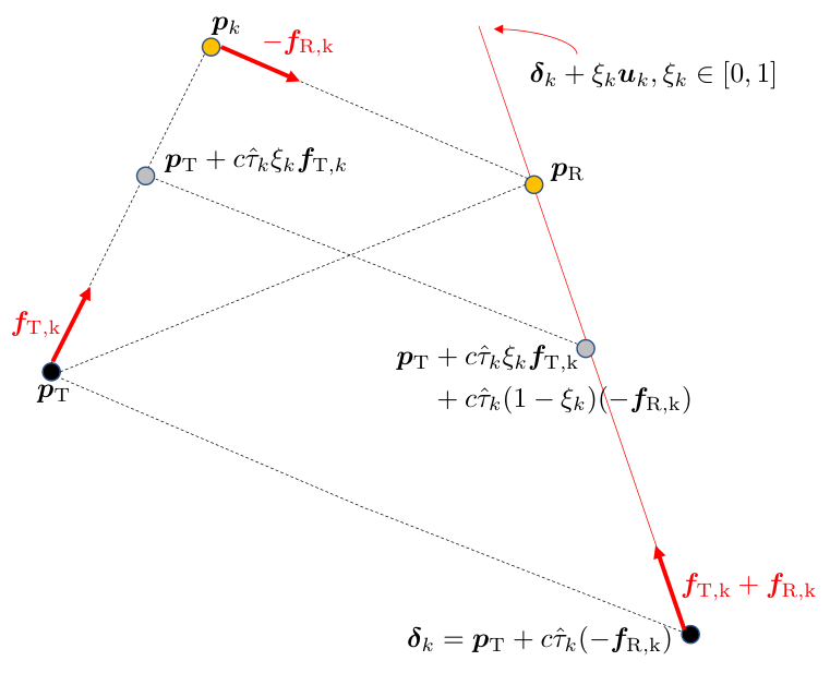
We present a general method based on [Wymeersch2018NLOS] that does not rely on knowledge on whether or not the LOS path is present. We define

which points along the direction of departure of path $k\in\{1,\ldots,\hat{P}\}$; and $\bm{f}_{\rm{R},k}$ is defined equivalently for the direction of arrival. For each cluster $k$ we can establish a relation to $\bm{p}_{\rm{R}}$ according to

with unknown $\xi_{k}\in[0,1]$. Note that for the LOS path (if it is present), the value of $\xi_{k}$ is arbitrary. In Fig. 2, we show the relation between the different defined vectors and the user location. Rearranging results in the line equation for each $k$ as

with $\bm{\delta}_{k}=\bm{p}_{\rm{T}}-c\hat{\tau}_{k}\bm{f}_{\mathrm{R},k}$ and $\bm{u}_{k}=c\hat{\tau}_{k}(\bm{f}_{\mathrm{T},k}+\bm{f}_{\mathrm{R},k})$. The intersection of these lines determines the estimate of $\bm{p}_{\rm{R}}$. Specifically, we consider the cost function

as sum of distance between $\bm{p}_{\rm{R}}$ and each path (35), and $\zeta_{k}\geq 0$ is the weight of the $k$-th path (e.g., dependent on the SNR or the spread of path). The least-squares solution becomes

with $\bar{\bm{u}}_{k}=\bm{u}_{k}/\|\bm{u}_{k}\|$.

Given $\hat{\bm{p}}_{\rm{R}}$, we can recover the scatter point $\bm{p}_{k}$ as intersection of the line equations $\bm{p}_{\rm{T}}+\zeta_{\rm{T}}\bm{f}_{\mathrm{T},k},\zeta_{\rm{T}}\in\mathbb{R}$ and $\bm{p}_{\rm{R}}+\zeta_{\rm{R}}\bm{f}_{\mathrm{R},k},\zeta_{\mathrm{R}}\in\mathbb{R}$ (see Fig. 2). The least-squares solution follows as

with $\bm{H}_{\mathrm{T},k}=\bm{I}-\bm{f}_{\mathrm{T},k}\bm{f}_{\mathrm{T},k}^{\mathsf{T}}$, $\bm{H}_{\mathrm{R},k}=\bm{I}-\bm{f}_{\mathrm{R},k}\bm{f}_{\mathrm{R},k}^{\mathsf{T}}$ and $\hat{\bm{p}}_{\rm{R}}$ from (37).

Note that the method does not require separation of specular and diffuse paths. The cost function in (36) can be applied with all $\hat{P}$ estimated paths, or only a selected subset of paths per cluster. In Section , the performance of different options will be compared.

In the case multiple users are to be localized simultaneously, the proposed method can be applied independently by each individual user, based on the received downlink signals, as is currently done in LTE. Different levels of cooperation can be envisioned, including map sharing [Kim2020] and exploiting inter-user correlations [Liu2020].

The most computationally demanding part of channel parameter estimation is the CP decomposition. In general, most CP decomposition algorithms, which factorize $R$-order tensors, face high computational cost due to computing gradients and (approximate) Hessians, line search and rotation. Table I in [Phan2013] summarizes the complexities of major computations in popular CP decomposition algorithms. For example, the alternating least squares (ALS) algorithm with line search has a complexity of order $\mathcal{O}\left(2^{R}PJ+RP^{3}\right)$, where $J=\prod_{r=1}^{R}M_{r}$ and $P$ denotes the total number of paths. Having $\hat{P}$ multipaths, estimation of $\hat{\bm{p}}_{\mathrm{R}}$ requires a single $3\times 3$ matrix inversion, followed by $\hat{P}+1$ matrix-vector multiplications. In addition, each scatter point estimate demands for a single $3\times 3$ matrix inversion plus three matrix-vector multiplications. Finally, estimation of $\hat{\bm{p}}_{\mathrm{R}}$ requires $\mathcal{O}(\hat{P})$ matrix-vector multiplications.

We consider a carrier frequency of 28 GHz, corresponding to $\lambda=1.07~\text{cm}$, a total bandwidth of 20 MHz with 100 subcarriers, of which 10 equally spaced subcarriers are used for pilots. A cyclic prefix of length 7 is used. 64 pilot OFDM symbols are sent, for a total duration of 3.52 ms. We set the pilots as $\mathbf{S}_{i}=\mathbf{I}$, $\forall i$. The surface reflection coefficient $\Gamma$ is not specified, as we only use diffuse paths.

As shown in Fig. , the transmitter and receiver are located at $\bm{p}_{\rm{T}}=[20,0,8]^{\mathsf{T}}$ and $\bm{p}_{\rm{R}}=[0,0,2]^{\mathsf{T}}$, respectively, and are surrounded by two surfaces: one building facade and a ground surface. The building facade’s center is at $[10,10,5]^{\mathsf{T}}$ with facade length of 20 m, facade height of 10 m, and orientation $[0,1,0]^{\mathsf{T}}$ ($x$-$z$ plane). The ground surface is at $[10,0,0]^{\mathsf{T}}$ with orientation $[0,0,1]^{\mathsf{T}}$ (reflected from ground, $x$-$y$ plane), surface dimension is $20\times 20$ m. Both surfaces are described as rough surfaces without specular component, using $L_{k}=100$ scatter points each. Furthermore, $K=2$ is assumed for the following simulations and all the resolved paths are utilized for positioning and mapping, unless stated otherwise.

The transmitter is equipped with a uniform rectangular array (URA) with ($8\times 8$) elements and placed along $y$-$z$ plane. In both directions, the inter-element spacing is $0.5\lambda$. The origin is the array reference point. The receiver is also equipped with a URA with ($8\times 8$) elements and placed along $y$-$z$ plane.

The Matlab package Tensorlab [tensorlab3.0] is utilized for tensor computation, which provides several core algorithms for the computation of the CP decomposition including optimization-based methods such as alternating least squares (ALS), unconstrained nonlinear optimization and nonlinear least squares (NLS). By default, NLS is used for the CP decomposition. It can handle the partially distinct channel parameter scenarios, which was also validated in [Wen2020].