∎
A posteriori error estimates in spaces for the Stokes system with Dirac measures Journal: Numerische MathematikThanks: FL is partially supported by CONICYT through FONDECYT Postdoctoral project 3190204. EO is partially supported by CONICYT through FONDECYT project 11180193. DQ is partially supported by USM through Programa de Incentivos a la Iniciación Científica (PIIC)
Abstract
We design and analyze a posteriori error estimators for the Stokes system with singular sources in suitable spaces. We consider classical low-order inf-sup stable and stabilized finite element discretizations. We prove, in two and three dimensional Lipschitz, but not necessarily convex polytopal domains, that the devised error estimators are reliable and locally efficient. On the basis of the devised error estimators, we design a simple adaptive strategy that yields optimal experimental rates of convergence for the numerical examples that we perform.
Keywords:
Stokes equations a posteriori error estimates Dirac measures adaptive finite elementsMSC
35Q35 76D07 35R06 65N15 65N50 76M101 Introduction
For , we let be an open and bounded polytopal domain in with Lipschitz boundary . The purpose of this work is the design and analysis of a posteriori error estimators for classical low-order inf-sup stable and stabilized finite element approximations of the Stokes problem
| (1) |
where corresponds to the Dirac delta supported at the interior point and . As it is customary in fluid mechanics, represents the velocity of the fluid, the pressure and is an externally applied force. Notice that, for simplicity, we have taken the viscosity to be equal to one. An instance of (1) appears in the modeling of active thin structures LACOUTURE2015187; FULFORD1986381; there the right hand side is a linear combination of Dirac deltas supported at interior points of . We also mention other applications such as the use of flagella by sessile organisms to generate feeding currents higdon79, modeling the flow of a fluid through structures with singular sources liron78; hasimoto59, slender body theories stephen81, improved models for the movement by cilia blake_1972, and optimal control of fluid flows 2019arXiv190711096F; 2018arXiv181002415A.
When the body force acting on the fluid and the mass production rate are smooth, the study of solution techniques for the Stokes and related models within a standard Hilbert space–based setting is well understood MR851383; MR2050138. However, recent models have emerged where the motion of an incompressible fluid is described by problem (1) or a small variation of it. Due to the singular nature of the body force , the problem must be understood in a completely different setting where the analysis of approximation techniques is scarce. Since is a Lipschitz polytope, the fact that , with , yields the existence of a unique solution with Larsson_Svensson; MR2987056; MR1386766. Here, denotes a positive constant that depends on . For a complete treatment of boundary value problems for the Stokes system on Lipschitz domains we refer the reader to MR2987056, where the authors prove optimal well–posedness results in all space dimensions and for all major types of boundary conditions.
Regarding the design and analysis of solution techniques for problem (1), and to the best of our knowledge, the first work that proposed an scheme is LACOUTURE2015187. Later, the authors of MR3854357 derived quasi–optimal local convergence results in . The authors operated under the assumption that the underlying domain is an open and bounded domain, or a square, and considered finite element discretizations based on the mini element and Taylor–Hood approximations. The error is analyzed on a subdomain which does not contain the singularity of the involved solution. On the other hand, in view of the fact that there is a Muckenhoupt weight related to the distance to such that , the authors of 2019arXiv190500476D; MR3892359 have operated within a weighted Sobolev space setting and derived a priori and a posteriori error estimates for classical low–order inf–sup stable finite element approximations.
Since is very singular, it is not expected for the pair , solution to (1), to have any global regularity properties beyond those inherited from the well–posedness of the problem. As a consequence, optimal error estimates for classical low–order inf–sup stable finite element approximations, such as the mini element and the lowest order Taylor–Hood element, cannot be expected. This motivates the design and analysis of adaptive finite element methods (AFEMs) for the efficient resolution of problem (1) since they are known to outperform classical FEM in practice and deliver optimal convergence rates when FEM cannot. AFEMs are a fundamental numerical tool in science and engineering that allow for the resolution of PDEs with relatively modest computational resources. An essential ingredient of an AFEM is an a posteriori error estimator. This is a computable quantity that depends on the discrete solution and data, and provides information about the local quality of the approximate solution. Therefore, it can be used for adaptive mesh refinement and coarsening, error control, and equidistribution of the computational effort. The a posteriori error analysis for linear second-order elliptic boundary value problems has attained a mature understanding MR1885308; MR2648380; MR3059294.
In contrast to the well-established theory for linear elliptic PDEs with smooth data, the a posteriori error analysis for finite element approximations of problems with singular forcing has not yet been fully understood. The main source of difficulty is the reduced regularity properties exhibited by the underlying solution. Within this context, the first work that provides an a posteriori error analysis for a finite element approximation of a Poisson problem with a Dirac delta as a forcing term is MR2262756. The authors of this work utilize suitable –norms and design, on a two dimensional setting, residual–type a posteriori error estimators. The devised estimators are proven to be reliable and locally efficient. We would like to also mention reference MR3237857 where the authors consider a posteriori error estimates for an electrostatics problem with a current dipole source and extend some of the results of MR2262756 to the three dimensional case. This is a singular problem, since the current dipole model involves first–order derivatives of a Dirac delta measure.
To the best of our knowledge, the only work that provides an advance concerning the a posteriori error analysis for the Stokes system (1) is MR3892359. In such a work, the authors propose a posteriori error estimators for classical low–order inf–sup stable and stabilized finite element approximations of the Stokes problem (1) in two and three dimensional Lipschitz polytopal domains. The authors operate within the setting of Muckenhoupt weighted Sobolev spaces and prove that the devised error estimators are reliable and locally efficient. In contrast, in this work we operate under a complete different setting; we make use of the fact that, since is Lipschitz , there exists such that with and devise a posteriori error estimator based on –norms. We consider the classical saddle point formulation of (1) and propose approximations based on popular low–order inf–sup stable and stabilized finite elements. For all these schemes, we devise a posteriori error estimators that are proven to be globally reliable and locally efficient when the approximation error is measured in suitable –norms. With the proposed estimators at hand, we also design simple adaptive strategies that yield optimal rates of convergence for the numerical examples that we perform.
The outline of this manuscript is as follows. In Section 2 we introduce the notation and functional framework we shall work with. In Section 3 we present a saddle point formulation for the Stokes system (1). We also review the well–posedness of the system and state regularity properties of its solution. In Section 4 we introduce classical low–order inf–sup stable finite element approximations of (1). The core of our work is Section 5, where we design a posteriori error estimators and obtain global reliability and local efficiency results. We extend, in Section 6, the results obtained in Section 5 to the case when stabilized finite element approximations are considered. Finally, in Section 7, we report numerical tests, in two and three dimensions, that illustrate the theory and exhibit the performance of the devised estimators.
2 Notation and preliminaries
Let us set notation and describe the setting we shall operate with.
Throughout this work, and is an open and bounded polytopal domain of with Lipschitz boundary . If and are normed vector spaces, we write to denote that is continuously embedded in . We denote by and the dual and the norm of , respectively.
Given , we denote by the real number such that , i.e., .
The relation indicates that , with a positive constant which is independent of a, b, and the size of the elements in the mesh. The value of might change at each occurrence.
3 The model problem
We begin with a motivation for the use of the spaces with .
3.1 Motivation
3.2 Saddle point formulation
3.3 Well–posedness
Our heuristic argument suggests that the well–posedness of problem (3) is conditioned to . To make matters precise, we introduce as the Green operator for the inhomogeneous problem for the incompressible Stokes system with vanishing Dirichlet boundary conditions. That is, if solves
then . The regularity results of (MR2987056, Corollary 1.7) (with and ) guarantee that the operator is bounded if
| (4) |
for some . As a consequence, for every bounded and Lipschitz domain , there exist such that is well–defined and bounded. When is a bounded and Lipschitz domain, the same conclusion holds for some .
We present the following result.
Theorem 3.1 (well–posedness)
Let and be an open and bounded Lipschitz polytope. There exists such that, if , then, problem (3) is well–posed. In addition,
where the hidden constant is independent of the solution and data.
Proof
We proceed on the basis of two cases.
- i)
- ii)
. Notice that . Analogous arguments to the ones presented in the previous case allow us to conclude that (3) is well–posed for .
This concludes the proof. ∎
3.4 Inf–sup condition
Let us introduce the product spaces
With these spaces at hand, we define the bilinear form by
| (5) |
with norm
| (6) |
4 Finite element approximation
We now introduce the discrete setting in which we will operate. We first introduce some terminology and a few basic ingredients and assumptions that will be common to all our methods.
4.1 Triangulation and finite element spaces
We consider to be a conforming partition of into closed simplices with size . Define . We denote by the collection of conforming and shape regular meshes that are refinements of an initial mesh .
Let be the set of internal dimensional interelement boundaries of . For , we denote by the diameter of . For , let denote the subset of which contains the sides in which are sides of . We also denote by the subset of that contains the two elements that have as a side, in other words, , where are such that . For , we define the stars or patches associated with an element as
| (8) |
For a discrete tensor valued function , we define the jump or interelement residual on the internal side , shared by the distinct elements , by . Here, and are unit normal on pointing towards and , respectively.
4.2 Inf–sup stable finite element spaces
We now introduce the inf–sup stable finite element spaces that will be considered in our work. Given a mesh , we denote by and the finite element spaces that approximate the velocity field and the pressure, respectively. The following elections are popular:
- (a)
The mini element (MR2050138, Section 4.2.4): Here,
where denotes the space spanned by local bubble functions.
- (b)
The lowest order Taylor–Hood element (MR2050138, Section 4.2.5): In this case,
(9) (10)
We observe that, for the values of provided in the statement of Theorem 3.1, we have and .
In the analysis that follows, the pair will represent indistinctly both the mini element and the lowest order Taylor–Hood element. An important property that these pairs of finite element spaces satisfy is the following compatibility condition: Let and let be the conjugate of . Then, there exists , independent of , such that
| (11) |
We refer the reader to (MR2050138, Lemma 4.20 and Lemma 4.24) for a proof.
4.3 Interpolation error estimates
For and , with , we define as the Lagrange interpolation operator onto continuous piecewise polynomials of degree over , that vanish on . We will consider for approximation based on mini element and for Taylor–Hood approximation. For , we set to be the Lagrange interpolation operator applied componentwise.
The following result provides interpolation error estimates.
Lemma 1 (interpolation error estimates)
Let . If , with , then
| (13) |
Let and . If , with , then
| (14) |
Proof
The estimate (13) is standard; see, for instance, (MR2050138, Theorem 1.103). The estimate (14) follows from the scaled–trace inequality
which follows, for instance, from the trace identity in (MR2648380, Lemma 6.2) and standard interpolation error estimates for the Lagrange interpolation operator (MR2050138, Theorem 1.103). This concludes the proof.∎
5 A posteriori error estimates
We begin our analysis by introducing the so–called residual. Let and be the solutions to problems (3) and (12), respectively. We define the residual as follows:
| (15) |
Notice that the residual depends on the approximated solution and the data and .
5.1 Error and residual
Let us define the error . The residual and the error are related by the following identity:
| (16) |
The next result guarantees that the residual and the error are equivalent.
Lemma 2 (equivalence result)
5.2 A posteriori error estimators
We now introduce a posteriori error estimators for the finite element approximation (12) on the basis of the low–order inf–sup stable finite element pairs introduced in Section 4.2.
Let . If is such that
- (i)
is not a vertex of or a midpoint of a side of , when Taylor–Hood approximation is considered, or
- (ii)
is not a vertex of , when the approximation based on the mini element is considered, then
we define the element error indicators
| (17) |
If and (i) or (ii) do not hold, then
| (18) |
If , then the indicator is defined as in (18). Here, denotes the solution to the discrete problem (12) and denotes the identity matrix in . We recall that we consider our elements to be closed sets. Notice that, when Taylor–Hood approximation is considered, for functions , with , we have that vanishes when is a vertex of or a midpoint of a side of . This motivates (i). Similar arguments motivate (ii); see also the proof of Theorem 5.1 below.
The a posteriori error estimators are thus defined by
| (19) |
5.3 Reliability
The main objective of this section is to obtain a global reliability property for the a posteriori error estimators .
Theorem 5.1 (global reliability)
Proof
We begin the proof by invoking the basic estimate , which follows immediately from Lemma 2. It thus suffices to bound . To accomplish this task, we notice that, in view of definitions (15) and (5), we have for arbitrary,
Next, we write , , and as integrals over elements and utilize elementwise integration by parts to arrive at
| (20) |
We invoke the relation , which follows from Galerkin orthogonality, to arrive at
| (21) |
Here, denotes the Lagrange interpolation operator; see Section 4.3 for details. We must immediately mention that, since , with , we have that . Consequently, is well–defined. We now bound each term on the right–hand side of (21) separately.
We estimate . Let such that . Notice that, if conditions (i) or (ii) do not hold, then vanishes. Assume that and conditions (i) or (ii) hold. If this is the case, standard interpolation error estimates for the Lagrange operator yields
The control of the term follows from Hölder’s inequality and (13). In fact, for , we have
The control of the term follows from a basic application of Hölder’s inequality: If , then
We now estimate the term . To accomplish this task, we first apply Hölder’s inequality and then the estimate (14). These arguments yield, for ,
5.4 Efficiency
In this section we study the efficiency properties of the a posteriori error estimators , defined in (19), by examining each of their contributions separately. To accomplish this task, we will invoke standard residual estimation techniques based in suitable bubble functions. Before proceeding with such analysis, we introduce the following notation: for an edge/face or triangle/tetrahedron , let be the set of vertices of . With this notation at hand, we define, for and , the standard element and edge bubble functions MR993474; MR3059294; MR1885308
respectively, where are the barycentric coordinates of . We recall that corresponds to the patch composed of the two elements of sharing .
We also introduce, inspired in (MR2262756, Section 3) and (MR3237857, Section 3), the following bubble functions. Given , we define as
| (22) |
Given , we define as
| (23) |
where denotes the interior of . We recall that the Dirac measure is supported at : it can thus be supported on the interior, an edge, or a vertex of an element of the triangulation .
Given , we introduce the continuation operator as defined in (MR1650051, Section 3). This operator maps polynomials onto piecewise polynomials of the same degree. With this operator at hand, we provide the following result.
Lemma 3 (bubble function properties)
Let , , , and . Then, the bubble functions and introduced in (22) and (23), respectively, satisfy
| (24) |
In addition, if and , then
| (25) | ||||
| (26) | ||||
| (27) |
Proof
Theorem 5.2 (local efficiency)
Let . Let be the solution to (3) and its finite element approximation obtained as the solution to (12). Then, for , the local error indicator , defined in (17)–(18), satisfies that
| (28) |
where is defined in (8). The hidden constant is independent of the solution , its approximation , the size of the elements in the mesh , and .
Proof
We proceed in five steps.
Step 1. Let . In this step we bound the term in (17)–(18). To accomplish this task and also to simplify the presentation of the material, we define and . We recall that is given as in (22). Now, set and in (20). This yields
Observe that . Now, set and in (16) and conclude that . We thus use (25) to derive
| (29) |
where, to obtain the last inequality, we have used Hölder’s inequality.
On the other hand, notice that
where denotes the transpose operator. We invoke the properties that satisfies, which are stated in Lemma 3, and standard inverse inequalities (MR2373954, Lemma 4.5.3) to arrive at
Replacing this estimate into (29) yields
| (30) |
Now, on the basis of the inverse estimate , (30) reveals that
| (31) |
This allows us to conclude that
| (32) |
Step 2. Let . The control of the term in (17)–(18) follows from the incompressibility condition . In fact,
| (33) |
Step 3. Let and . We bound in (17)–(18). To simplify the presentation of the material, we define
Set and in (16) and invoke (20). This yields
We recall that . We now use that and invoke estimate (26) and Hölder’s inequality, to arrive at
| (34) |
This estimate in conjunction with (31) and an inverse inequality yield
We now notice that . This implies that
We thus invoke the estimate , which follows from a scaled–trace inequality and an inverse estimate, to arrive at
This and allow us to arrive at
| (35) |
Step 4. Let . In this step we bound the remaining term in (17). If , then the desired estimate (28) follows directly from (32), (33), and (35). If , and (i) and (ii) hold, the indicator contains the term . To control this term, we invoke the smooth function , whose construction we owe to (MR2262756, Section 3) and is such that
We also have the properties
| (36) |
With this smooth function at hand, we define . Here, the involved operations, i.e., the power, the absolute value and the sign function, must be understood componentwise. Define
Set and in (16). Invoke the identity (20) to arrive at
Invoking Hölder’s inequality and suitable estimates for the function , which are stated in (36), we obtain that
In view of (31) and (35), we arrive at the desired estimate
| (37) |
Step 5. Finally, by gathering the estimates (32), (33), (35), and (37) we arrive at the desired local lower bound (28).∎
6 A stabilized scheme
In Section 5 we have designed and analyzed a posteriori error estimators for classical low–order inf–sup stable finite element approximations of problem (3); the involved pairs of finite elements satisfy the compatibility condition (11), which comes with a cost. This condition requires to increase the polynomial degree of the discrete spaces beyond what is required for conformity. If lowest order possible is desired, it is thus necessary to modify the discrete problem to circumvent the need of satisfying condition (11). This gives rise to the so–called stabilized finite element methods. Several stabilized techniques are available in the literature. For an extensive review of different stabilized finite element methods we refer the reader to (MR2454024, Part IV, Section 3), (MR2490235, Chapter 7) and (MR3561143, Chapter 4).
We now describe the low–order stabilized schemes that we will consider in our work. To present them, we introduce the finite element spaces
| (38) |
and
| (39) |
where . With these spaces at hand, we propose the following stabilized finite element method: Find such that
| (40) |
where and are defined by
and
respectively. Here, , , and correspond to stabilization parameters. The well–posedness of problem (40) follows from (MR2454024, Lemma 3.4, Section 3.1), when , and (MR1740398, Section 2.1), when and , in conjunction with the equivalence of norms on discrete spaces.
We must immediately notice that, in view of the stabilization terms and in problem (40), the Galerkin orthogonality is no longer valid. Instead, we have the following relation for :
We recall that denotes the residual and is defined in (16). For , the previous relation can be rewritten as
| (41) |
We now introduce local error indicators and a posteriori error estimators. Let . If is such that is not a vertex of , we define the element error indicators
| (42) |
If is a vertex of , then
| (43) |
If , then the indicator is defined as in (43). Here, denotes the solution to the stabilized discrete problem (40) and denotes the identity matrix in . We recall that we consider our elements to be closed sets.
The a posteriori error estimators are thus defined by
| (44) |
We now derive global reliability and local efficiency properties for the error estimators .
Theorem 6.1 (reliability and local efficiency)
Proof
We first derive the reliability estimate (45). To accomplish this task, we first observe, from (41), that
where denote the Lagrange interpolation operator of Section 4.3.
A simple inspection of the right–hand side of the previous expression reveals that, with the exception , all the involved terms have been estimated in the proof of Theorem 5.1. To control we proceed as follows:
We thus invoke the stability of the Lagrange interpolation operator (MR2050138, Theorem 1.103) to arrive at
This estimate combined with the estimates obtained in the proof of Theorem 5.1 yield (45).
7 Numerical Experiments
We conduct a series of numerical examples that illustrate the performance of the devised a posteriori error estimators. To explore the performance of the estimators , defined in (19), we consider the discrete system (12) with the discrete spaces (9) and (10). This setting will be referred to as Taylor–Hood approximation. The performance of the error estimators , defined in (44), is explored by solving the stabilized discrete system (40) with the following finite element setting: the discrete spaces are (38) and (39), with , and the stabilization parameters are , , and . This setting will be referred to as low–order stabilized approximation.
7.1 Implementation
All the experiments have been carried out with the help of a code that we implemented using C++. All matrices have been assembled exactly. The right hand sides of the assembled systems, the local indicators, and the approximation errors, are computed by a quadrature formula which is exact for polynomials of degree for two dimensional domains and degree for three dimensional domains. The linear systems were solved using the multifrontal massively parallel sparse direct solver (MUMPS) MUMPS1; MUMPS2.
For a given partition we seek that solves the discrete system (12) or the stabilized discrete scheme (40). We thus compute the local error indicators or to drive the adaptive procedure described in Algorithm 1 and compute the global error estimators or in order to assess the accuracy of the approximation. A sequence of adaptively refined meshes is thus generated from the initial meshes shown in Figure 1. For Taylor–Hood approximation, the total number of degrees of freedom is , where is given by (9)–(10). For low–order stabilized approximation, , where is given by (38)–(39) with . The error is measured in the norm .


In the experiments that we perform we go beyond the presented theory and include a series of Dirac delta sources on the right–hand side of the momentum equation. To make matters precise, we will replace the momentum equation in (1) by
where corresponds to a finite ordered subset of with cardinality and . We thus propose the following a posteriori error estimator when Taylor–Hood approximation is considered:
For each , the local error indicators are given by: If and (i) or (ii) hold, then
| (47) |
If and (i) or (ii) do not hold, then
| (48) |
If , then the indicator is defined as in (48). Notice that, when , the total error estimator coincides with , which is defined in (19).
Similarly, when the low–order stabilized approximation scheme is considered, we propose the error estimator
For each , the local error indicators are given by: If is such that is not a vertex of , then
| (49) |
If is a vertex of , then
| (50) |
If , then the indicator is defined as in (50).
In the following numerical examples, when it corresponds, we replace by and by in Algorithm 1.
We consider problems with homogeneous boundary conditions whose exact solutions are not known. We also consider problems with inhomogeneous Dirichlet boundary conditions whose exact solutions are known. Notice that this violates the assumption of homogeneous Dirichlet boundary conditions which is needed for the analysis that we have performed. In this case, we write the solution in terms of fundamental solutions of the Stokes equations (MR2808162, Section IV.2):
| (51) |
where, if and is the identity matrix in , then
denotes the canonical basis of .
7.2 Taylor–Hood approximation
We perform two and three dimensional examples on convex and nonconvex domains and with different number of source points.
Example 1 (Convex domain). We consider and
The solution is given as in (51).
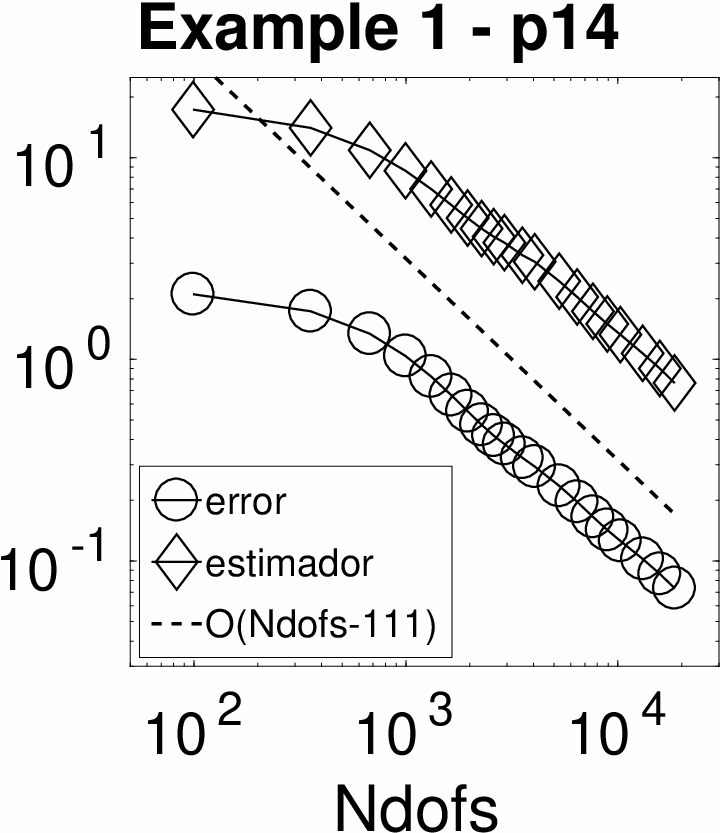
In this example we investigate the effect of varying the integrability index . Notice that, since problem (3) is well–posed for , the solution belongs to for every . In the particular setting of Example 1, we will thus consider . Finally, for each integrability index , we compute the effectivity index .
In Figures 2 and 3 we present the results obtained for Example 1. In particular, Figure 2 presents, for different values of the integrability index , experimental rates of convergence for and , effectivity indices , and adaptively refined meshes. We observe, in subfigures (A.1)–(D.1), optimal experimental rates of convergence for the error estimators and the total error . In subfigures (A.3)–(D.3), we appreciate the effect of varying the integrability index on the adaptively refined meshes. In particular, we observe that the adaptive refinement is mostly concentrated on the points where the Dirac measures are supported. We also observe that the effectivity indices decrease as the index increases; see subfigures (A.2)–(D.2). Finally, all the effectivity indices are stabilized around values between 6 and 13. This shows the accuracy of the proposed a posteriori error estimators when used in the adaptive loop described in Algorithm 1. In Figure 3 we present experimental rates of convergence for and for uniform and adaptive refinement when . From subfigures (A)–(B) we observe that the devised adaptive loop outperforms uniform refinement. Moreover, adaptive refinement exhibits an optimal experimental rate of convergence.
Example 2 (L-shaped domain). We let , , , and
In Figure 4 we report the results obtained for Example 2. We present the finite element approximations of and , experimental rates of convergence for the error estimators , and adaptively refined meshes. We observe, in subfigure (A), that, for all the values of , optimal experimental rates of convergence for the total error estimators are attained. We also observe, in the adaptively refined meshes (D)–(F), that the refinement is being concentrated around the re–entrant corner and the source points ().

(A.1)
(B.1)

(C.1)

(D.1)

(A.2)

(B.2)

(C.2)

(D.2)

(A.3)

(B.3)

(C.3)

(D.3)

(A)

(B)

(A)

(B)

(C)

(D)

(E)

(F)
Remark 1 (Influence of on )
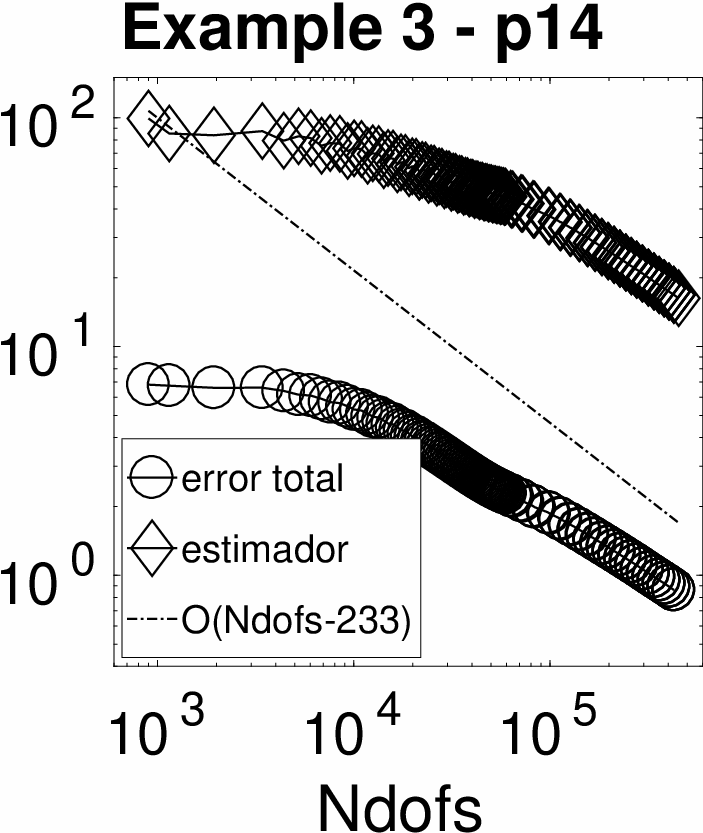
In Figure 2, we present experimental rates of convergence for the estimators and the total error for different values of the integrability index . Notice that, each plot involves a different range of numbers of degrees of freedom. The reported numerical results suggest that this may be due to the fact that the adaptive refinement depends on the value of : as increases, the refinement is mostly performed on the elements that are close to the Dirac measure points; see Figure 2 (A.3)–(D.3). When gets close to , after a certain number of adaptive iterations, there are elements , around the singular points, such that . As a consequence, the assembly calculations reach machine precision numbers and thus make impossible more computations within the adaptive procedure. The same behavior is observed in Figure 4 (A), where for each value of the estimator involves a different range of numbers of degrees of freedom.
We now present a three dimensional example with inhomogeneous Dirichlet boundary conditions.
Example 3 (Convex domain). In this case we consider and
The solution for this example corresponds to the one described in (51).
In Figure 5 we report the results obtained for Example 3. We present, for different values of the integrability index , experimental rates of convergence for and and adaptively refined meshes. We observe in subfigures (A.1)–(D.1), optimal experimental rates of convergence for the error estimators and the total error . In subfigures (A.2)–(D.2), we observe the effect of varying the integrability index on the adaptively refined meshes. In particular, we appreciate that the adaptive refinement is mostly concentrated on the points where the Dirac measures are supported.


(A.1) (A.2)


(B.1) (B.2)


(C.1) (C.2)

(D.1) (D.2)
7.3 A stabilized scheme
We perform numerical experiments for low–order stabilized approximation with the discrete spaces (38) and (39), taking , and the stabilization parameters , , and .
Example 4 (L-shaped domain). We let , , , and .
We report in Figure 6 the results obtained for Example 4. We present the finite element approximations of and , experimental rates of convergence for the error estimators and adaptively refined meshes. We observe in subfigure (A), that an optimal experimental rate of convergence for the total error estimator is attained. We also observe in the adaptively refined meshes (D)–(E), that the refinement is being concentrated around the re–entrant corner and the source point.

(A)

(B)

(C)

(D)

(E)
Example 5 (Convex domain). We let , ,
and
In Figure 7 we report the results obtained for Example 5. We observe in subfigure (A), that an optimal experimental rate of convergence for the total error estimator is attained. On the other hand, it is clear in the adaptively refined mesh (B), that the adaptive refinement is mostly concentrated on the points where the Dirac measures are supported.

(A)
(B)
7.4 Conclusions.
We present the following conclusions.
-
Most of the refinement occurs near to where the Dirac measures are located. This attests to the efficiency of the devised estimators. When the domain involves geometric singularities, refinement is also being performed in regions that are close to them. This shows a competitive performance of the a posteriori error estimators.
-
The numerical experiments suggest that a small value of delivers the best results.
-
In spite of the very singular nature of the problem (1), our proposed estimators are able to deliver optimal experimental rates of convergence within an adaptive loop.
References
- (1) M. Ainsworth and J. T. Oden, A posteriori error estimation in finite element analysis, Pure and Applied Mathematics (New York), Wiley-Interscience [John Wiley & Sons], New York, 2000.
- (2) A. Allendes, F. Fuica, E. Otárola, and D. Quero, An adaptive FEM for the pointwise tracking optimal control problem of the Stokes equations, SIAM J. Sci. Comput., 41 (2019), pp. A2967–A2998.
- (3) A. Allendes, E. Otárola, and A. J. Salgado, A posteriori error estimates for the Stokes problem with singular sources, Comput. Methods Appl. Mech. Engrg., 345 (2019), pp. 1007–1032.
- (4) A. Alonso Rodríguez, J. Camaño, R. Rodríguez, and A. Valli, A posteriori error estimates for the problem of electrostatics with a dipole source, Comput. Math. Appl., 68 (2014), pp. 464–485.
- (5) P. Amestoy, I. Duff, and J.-Y. L’Excellent, Multifrontal parallel distributed symmetric and unsymmetric solvers, Computer Methods in Applied Mechanics and Engineering, 184 (2000), pp. 501 – 520.
- (6) P. R. Amestoy, I. S. Duff, J.-Y. L’Excellent, and J. Koster, A fully asynchronous multifrontal solver using distributed dynamic scheduling, SIAM J. Matrix Anal. Appl., 23 (2001), pp. 15–41 (electronic).
- (7) R. Araya, E. Behrens, and R. Rodríguez, A posteriori error estimates for elliptic problems with Dirac delta source terms, Numer. Math., 105 (2006), pp. 193–216.
- (8) C. Bernardi, C. Canuto, and Y. Maday, Generalized inf-sup conditions for Chebyshev spectral approximation of the Stokes problem, SIAM J. Numer. Anal., 25 (1988), pp. 1237–1271.
- (9) S. Bertoluzza, A. Decoene, L. Lacouture, and S. Martin, Local error analysis for the Stokes equations with a punctual source term, Numer. Math., 140 (2018), pp. 677–701.
- (10) J. Blake, A model for the micro-structure in ciliated organisms, Journal of Fluid Mechanics, 55 (1972), p. 1–23.
- (11) P. B. Bochev and M. D. Gunzburger, Least-squares finite element methods, vol. 166 of Applied Mathematical Sciences, Springer, New York, 2009.
- (12) S. C. Brenner and L. R. Scott, The mathematical theory of finite element methods, vol. 15 of Texts in Applied Mathematics, Springer, New York, third ed., 2008.
- (13) R. M. Brown and Z. Shen, Estimates for the Stokes operator in Lipschitz domains, Indiana Univ. Math. J., 44 (1995), pp. 1183–1206.
- (14) S. Childress, Mechanics of swimming and flying, vol. 2 of Cambridge Studies in Mathematical Biology, Cambridge University Press, Cambridge-New York, 1981.
- (15) R. G. Durán, E. Otárola, and A. J. Salgado, Stability of the Stokes projection on weighted spaces and applications, arXiv e-prints, (2019), p. arXiv:1905.00476.
- (16) A. Ern and J.-L. Guermond, Theory and practice of finite elements, vol. 159 of Applied Mathematical Sciences, Springer-Verlag, New York, 2004.
- (17) F. Fuica, E. Otárola, and D. Quero, Error estimates for optimal control problems of the Stokes system with Dirac measures, arXiv e-prints, (2019), p. arXiv:1907.11096.
- (18) G. Fulford and J. Blake, Muco-ciliary transport in the lung, Journal of Theoretical Biology, 121 (1986), pp. 381 – 402.
- (19) G. P. Galdi, An introduction to the mathematical theory of the Navier-Stokes equations, Springer Monographs in Mathematics, Springer, New York, second ed., 2011. Steady-state problems.
- (20) V. Girault and P.-A. Raviart, Finite element methods for Navier-Stokes equations, vol. 5 of Springer Series in Computational Mathematics, Springer-Verlag, Berlin, 1986. Theory and algorithms.
- (21) H. Hasimoto, On the periodic fundamental solutions of the Stokes’ equations and their application to viscous flow past a cubic array of spheres, J. Fluid Mech., 5 (1959), pp. 317–328.
- (22) J. J. L. Higdon, The generation of feeding currents by flagellar motions, J. Fluid Mech., 94 (1979), pp. 305–330.
- (23) V. John, Finite element methods for incompressible flow problems, vol. 51 of Springer Series in Computational Mathematics, Springer, Cham, 2016.
- (24) D. Kay and D. Silvester, A posteriori error estimation for stabilized mixed approximations of the Stokes equations, SIAM J. Sci. Comput., 21 (1999/00), pp. 1321–1336.
- (25) L. Lacouture, A numerical method to solve the Stokes problem with a punctual force in source term, Comptes Rendus Mécanique, 343 (2015), pp. 187–191.
- (26) S. Larsson and E. D. Svensson, Pointwise a posteriori error estimates for the Stokes equations in polyhedral domains, Preprint, (2006).
- (27) N. Liron and R. Shahar, Stokes flow due to a Stokeslet in a pipe, J. Fluid Mech., 86 (1978), pp. 727–744.
- (28) M. Mitrea and M. Wright, Boundary value problems for the Stokes system in arbitrary Lipschitz domains, Astérisque, (2012), pp. viii+241.
- (29) R. H. Nochetto, K. G. Siebert, and A. Veeser, Theory of adaptive finite element methods: an introduction, in Multiscale, nonlinear and adaptive approximation, Springer, Berlin, 2009, pp. 409–542.
- (30) H.-G. Roos, M. Stynes, and L. Tobiska, Robust numerical methods for singularly perturbed differential equations, vol. 24 of Springer Series in Computational Mathematics, Springer-Verlag, Berlin, second ed., 2008. Convection-diffusion-reaction and flow problems.
- (31) R. Verfürth, A posteriori error estimators for the Stokes equations, Numer. Math., 55 (1989), pp. 309–325.
- (32) R. Verfürth, A posteriori error estimators for convection-diffusion equations, Numer. Math., 80 (1998), pp. 641–663.
- (33) R. Verfürth, A posteriori error estimation techniques for finite element methods, Numerical Mathematics and Scientific Computation, Oxford University Press, Oxford, 2013.