Analysing Deep Reinforcement Learning Agents Trained with Domain Randomisation
Abstract
Deep reinforcement learning has the potential to train robots to perform complex tasks in the real world without requiring accurate models of the robot or its environment. A practical approach is to train agents in simulation, and then transfer them to the real world. One popular method for achieving transferability is to use domain randomisation, which involves randomly perturbing various aspects of a simulated environment in order to make trained agents robust to the reality gap. However, less work has gone into understanding such agents—which are deployed in the real world—beyond task performance. In this work we examine such agents, through qualitative and quantitative comparisons between agents trained with and without visual domain randomisation. We train agents for Fetch and Jaco robots on a visuomotor control task and evaluate how well they generalise using different testing conditions. Finally, we investigate the internals of the trained agents by using a suite of interpretability techniques. Our results show that the primary outcome of domain randomisation is more robust, entangled representations, accompanied with larger weights with greater spatial structure; moreover, the types of changes are heavily influenced by the task setup and presence of additional proprioceptive inputs. Additionally, we demonstrate that our domain randomised agents require higher sample complexity, can overfit and more heavily rely on recurrent processing. Furthermore, even with an improved saliency method introduced in this work, we show that qualitative studies may not always correspond with quantitative measures, necessitating the combination of inspection tools in order to provide sufficient insights into the behaviour of trained agents.
keywords
Deep reinforcement learning, Generalisation, Interpretability, Saliency1 Introduction
Deep reinforcement learning (DRL) is currently one of the most prominent subfields in AI, with applications to many domains (Arulkumaran et al. 2017; François-Lavet et al. 2018). One of the most enticing possibilities that DRL affords is the ability to train robots to perform complex tasks in the real world, all from raw sensory inputs. For instance, while robotics has traditionally relied on hand-crafted pipelines, each performing well-defined estimation tasks – such as ground-plane estimation, object detection, segmentation and classification, (Kragic and Vincze 2009; Martinez-Gomez et al. 2014) – it is now possible to learn visual perception and control in an “end-to-end” fashion (Levine et al. 2016; Gu et al. 2017; Zhu et al. 2017; Levine et al. 2018), without explicit specification and training of networks for specific sub-tasks.
A major advantage of using reinforcement learning (RL) versus the more traditional approach to robotic system design based on optimal control is that the latter requires a transition model for the task in order to solve for the optimal sequence of actions. While optimal control, when applicable, is more efficient, modelling certain classes of objects (e.g., deformable objects) can require expensive simulation steps, and often physical parameters (e.g., frictional coefficients) of real objects that are not known in detail. Instead, approaches that use RL can learn a direct mapping from observations to the optimal sequence of actions, purely through interacting with the environment. Through the powerful function approximation capabilities of neural networks (NNs), deep learning (DL) has allowed RL algorithms to scale to domains with significantly more complex input and action spaces than previously considered tractable.

The downside is that while DRL algorithms can learn complex control policies from raw sensory data, they typically have poor sample complexity. In practice, this means training DRL algorithms in simulators before deploying them on real robots, which then introduces a reality gap (Jakobi et al. 1995) between the simulated and real worlds—including not just differences in physics, but also visual appearance. There are several solutions to this problem, including fine-tuning a DRL agent on the real world (Rusu et al. 2017), performing system identification to reduce the domain gap (Chebotar et al. 2018), and explicitly performing domain adaptation (Tzeng et al. 2015; Bousmalis et al. 2018).
One solution to increase the robustness of agents to potential differences between simulators and the real world is to use domain randomisation (DR; pictured in Figure 1), in which various properties of the simulation are varied, altering anything from the positions or dynamical properties of objects to their visual appearance. This extension of data augmentation to RL environments has been used to successfully train agents for a range of different robots, including robotic arms (Tobin et al. 2017; James et al. 2017), quadcopters (Sadeghi and Levine 2017), and even humanoid robotic hands (Andrychowicz et al. 2018). While early uses of DR (Tobin et al. 2017; James et al. 2017) did not include transition dynamics as a random property, we note that “dynamics randomisation” (Peng et al. 2018) can now also be considered part of the standard DR pipeline. Common practice is to design DR to incorporate as many variations as possible, such that the real world would, ideally, be a “subset” of the set of DR environments.
When the primary aim of this line of research is to enable the training of agents that perform well in the real world, there is an obvious need to characterise how these agents behave before they can be deployed “in the wild”. In particular, one can study how well these agents generalise—a criterion that has received considerable interest in the DRL community recently (Zhang et al. 2018a; Zhang et al. 2018b; Justesen et al. 2018; Witty et al. 2018; Packer et al. 2018; Cobbe et al. 2018; Zhao et al. 2019). To do so, we can construct unit tests that not only reflect the conditions under which the agent has been trained, but also extrapolate beyond; for instance, James et al. (James et al. 2017) studied the test-time performance of agents trained with DR in the presence of distractors or changed illumination. While adding robustness to these extrapolation tests can be done by simply training under the new conditions, we are interested in developing general procedures that would still be useful when this option is not available. As we show later (in Subsection 3.3), depending on the training conditions, we can even observe a failure of agents trained with DR to generalise to the much simpler default visuals of the simulator.
While unit tests provide a quantitative measure by which we can probe the performance of trained agents under various conditions, they treat the trained agents as black boxes. However, with full access to the internals of the trained models and even control over the training process, we can dive even further into the models. Using common interpretability tools such as saliency maps (Morch et al. 1995; Simonyan et al. 2013; Zeiler and Fergus 2014; Selvaraju et al. 2017; Sundararajan et al. 2017) and dimensionality reduction methods (Pearson 1901; Maaten and Hinton 2008; McInnes et al. 2018) for visualising NN activations (Rauber et al. 2017), we can obtain information on why agents act the way they do. The results of these methods work in tandem with unit tests, as matching performance to the qualitative results allows us to have greater confidence in interpreting the latter; in fact, this process allowed us to debug and improve upon an existing saliency map method, as detailed in Subsection 4.1. Through a combination of existing and novel methods, we present here a more extensive look into DRL agents that have been trained to perform control tasks using both visual and proprioceptive inputs. In particular, under our set of experimental conditions, we show that our agents trained with visual DR:
- •
require more representational learning capacity (Subsection 4.5),
- •
are more robust to visual changes in the scene, exhibiting generalisation to unseen local/global perturbations (Subsection 3.4),
- •
use a smaller set of more reliable visual cues when not provided proprioceptive inputs (Subsection 4.1),
- •
more heavily rely on recurrent processing (Subsection 4.6),
- •
- •
learn more robust (Subsection 4.4) and entangled (Frosst et al. 2019) representations (Subsection 4.7),
- •
and can “overfit” to DR visuals (Subsection 3.3).
2 Methods
2.1 Reinforcement Learning
In RL, the aim is to learn optimal behaviour in sequential decision problems (Sutton and Barto 2018), such as finding the best trajectory for a manipulation task. It can formally be described by a Markov decision process (MDP), whereby at every timestep the agent receives the state of the environment , performs an action sampled from its policy (potentially parameterised by weights ), and then receives the next state along with a scalar reward . The goal of RL is to find the optimal policy, , which maximises the expected return:
where in practice a discount value is used to weight earlier rewards more heavily and reduce the variance of the return over an episode of interaction with the environment, ending at timestep .
Policy search methods, which are prevalent in robotics (Deisenroth et al. 2013), are one way of finding the optimal policy. In particular, policy gradient methods that are commonly used with NNs perform gradient ascent on to optimise a parameterised policy (Williams and Peng 1991). Other RL methods rely on value functions, which represent the future expected return from following a policy from a given state: . The combination of learned policy and value functions are known as actor-critic methods, and utilise the critic (value function) in order to reduce the variance of the training signal to the actor (policy) (Barto et al. 1983). Instead of directly maximising the return , the policy can then be trained to maximise the advantage (the difference between the empirical and predicted return).
We note that in practice many problems are better described as partially-observed MDPs, where the observation received by the agent does not contain full information about the state of the environment. In visuomotor object manipulation this can occur as the end effector blocks the line of sight between the camera and the object, causing self-occlusion. A common solution to this is to utilise recurrent connections within the NN, allowing information about observations to propagate from the beginning of the episode to the current timestep (Wierstra et al. 2007).
2.1.1 Proximal Policy Optimisation
For our experiments we train our agents using proximal policy optimisation (PPO) (Schulman et al. 2017), a widely used and performant RL algorithm.11 1 In particular, PPO has been used with DR to train a policy that was applied to a Shadow Dexterous Hand in the real world (Andrychowicz et al. 2018). Rather than training the policy to maximise the advantage directly, PPO instead maximises the surrogate objective:
with
where is the ratio between the current policy and the old policy, is the clip ratio which restricts the change in the policy distribution, and is the advantage, which we choose to be the Generalised Advantage Estimate (GAE):
that mixes Monte Carlo returns and temporal difference errors with hyperparameter (Schulman et al. 2015).
In practice, both the actor and the critic can be combined into a single NN with two output heads, parameterised by (Mnih et al. 2016). The full PPO objective involves maximising , minimising the squared error between the learned value function and the empirical return:
and maximising the (Shannon) entropy of the policy, which for discrete action sets of size , is defined as:
Entropy regularisation prevents the policy from prematurely collapsing to a deterministic solution and aids exploration (Williams and Peng 1991).
Using a parallelised implementation of PPO, we are able to train our agents to strong performance on all training setups within a reasonable amount of time. Training details are described in Subsection 3.2.
2.2 Neural Network Interpretability
The recent success of machine learning (ML) methods has led to a renewed interest in trying to interpret trained models, whereby an explanation of a model’s “reasoning” may be used as a way to understand other properties, such as safety, fairness, reliability, or simply to provide an explanation of the model’s behaviour (Doshi-Velez and Kim 2017). In this work, we are primarily concerned with scientific understanding, but our considerations are grounded in other properties necessary for eventual real-world deployment, such as robustness.
The challenge that we face is that, unlike other ML algorithms that are considered interpretable by design (such as decision trees or nearest neighbours (Freitas 2014)), standard NNs are generally considered black boxes. However, given decades of research into methods for interpreting NNs (Morch et al. 1995; Craven and Shavlik 1996), we now have a range of techniques at our disposal (Guidotti et al. 2018). Beyond simply looking at test performance (a measure of interpretability in its own right (Doshi-Velez and Kim 2017)), we will focus on a variety of techniques that will let us examine trained NNs both in the context of, and independently of, task performance. In particular, we discuss saliency maps (Subsection 4.1), activation maximisation (Subsection 2.2.2), weight visualisations (Subsection 2.2.3), statistical and structural weight characterisations (Subsection 2.2.4), unit ablations (Subsection 2.2.5), layer re-initialisation (Subsection 2.2.6) and activation analysis (Subsection 2.2.8). By utilising a range of techniques we hope to cover various points along the trade-off between fidelity and interpretability (Ribeiro et al. 2016).
2.2.1 Saliency Maps
Saliency maps are one of the most common techniques used for understanding the decisions made by NNs, and in particular, convolutional NNs (CNNs). The most common methods are gradient-based, and utilise the derivative of the network output with respect to the inputs, indicating, for images, how changing the pixel intensities at each location will affect the output (Simonyan et al. 2013). We investigated the use of two popular, more advanced variants of this technique—gradient-weighted class activation mapping (Grad-CAM) (Selvaraju et al. 2017) and integrated gradients (IG) (Sundararajan et al. 2017)—as well as an occlusion-based method, which masks parts of the image and performs a sensitivity analysis with respect to the change in the network’s outputs (Zeiler and Fergus 2014). As shown in Figure 2, the latter technique gave the most ‘‘interpretable’’ saliency maps across all trained agents, so we utilise it alone when analysing our trained agents in latter sections.22 2 This observation is also in line with prior work on interpreting DRL agents (Greydanus et al. 2018). In light of the unreliability of saliency methods (Kindermans et al. 2017), we include a discussion and comparison of these methods to illuminate the importance of checking the outputs of qualitative methods. As a final remark we note that clustering methods have been used to automatically find groups of strategies via collections of saliency maps (Lapuschkin et al. 2019), but, given the relative visual simplicity of our tasks, highlighting individual examples is sufficiently informative.


CAM
The class average map (CAM) (Zhou et al. 2016) was developed as a saliency method for CNNs with global average pooling (Lin et al. 2013) trained for the purpose of object recognition. The value of the saliency map for class at spatial location is calculated by summing over the activations of the final convolutional layer (with channels) and the corresponding class weights :
Grad-CAM
Given a network and input , Grad-CAM extends CAM from fully-convolutional NNs to generic CNNs by instead constructing class weights by using the partial derivative for the output of a class , , with respect to the feature maps of any convolutional layer. The Grad-CAM saliency map for a class, , is the positive component of the linear combination of class weights and feature maps :
where is formed by averaging over spatial locations .
In place of a given class , we use Grad-CAM to create a saliency map per (output) action (Figure 3). As in this case, it is not always clear how to interpret Grad-CAM saliency maps for our trained agents. There are many reasons such techniques might “fail”, such as the mixing of both positive and negative contributions towards the network outputs (Springenberg et al. 2015; Bach et al. 2015).


Integrated Gradients
Sundarajan et al. (Sundararajan et al. 2017) proposed that attribution methods (saliency maps in our case) should be:
- Sensitive
-
If an input and the baseline differ in one feature and have different outputs, the differing feature should have a non-zero attribution
- Invariant to implementation
-
Attributions should be identical for two functionally equivalent models
Prior gradient-based methods break the first property. Their method, IG, achieves both by constructing the saliency value for each input dimension from the path integral of the gradients along the linear interpolation between input and a baseline input :
Although Sundarajan et al. (Sundararajan et al. 2017) suggested that a black image can be used as the baseline, we found that using the (dataset) average input, provided superior results. Contemporaneous work has examined the use of more advanced baselines for gradient-based saliency map methods (Sturmfels et al. 2020).
Occlusion
As an alternative to gradient-based methods, Zeiler et al. (Zeiler and Fergus 2014) proposed running a (grey, square) mask over the input and tracking how the network’s outputs change in response. Greydanus et al. (Greydanus et al. 2018) applied this method to understanding actor-critic-based DRL agents, using the resulting saliency maps to examine strong and overfitting policies; they however noted that a grey square may be perceived as part of a grey object, and instead used a localised Gaussian blur to add ‘‘spatial uncertainty’’. The saliency value for each input location is the Euclidean distance between the original output33 3 In practice taken to be the logits for a categorical policy. We considered that the Kullback-Leibler divergence between policy distributions might be more meaningful, but found that it produces qualitatively similar saliency maps. and the output given the input which has been occluded at location :
where denotes the -norm.
However, we found that certain trained agents sometimes confused the blurred location with the target location—a failing of the attribution method against noise/distractors (Kindermans et al. 2016), and not necessarily the model itself. Motivated by the methods that compute interpretations against reference inputs (Bach et al. 2015; Ribeiro et al. 2016; Shrikumar et al. 2017; Sundararajan et al. 2017; Lundberg and Lee 2017), we replaced the Gaussian blur with a mask44 4 Replacing a circular region of 5px radius around the location. derived from a baseline input, which roughly represents what the model would expect to see on average. Intuitively, this acts as a counterfactual, revealing what would happen if the specific part of the input was not there. For this we averaged over frames collected from our standard evaluation protocol (see Subsection 3.1 for details), creating an average input to be used as an improved baseline for IG, as well as the source of the mask for the occlusion-based method (Figure 4). Unless specified otherwise, we use our average input baseline for all IG and occlusion-based saliency maps.


2.2.2 Activation Maximisation
Gradients can also be used to try and visualise what maximises the activation of a given neuron/channel. This can be formulated as an optimisation problem, using projected55 5 After every gradient step the input is clamped back to within . gradient ascent in the input space (Erhan et al. 2009). Although this would ideally show what a neuron/channel is selective for, unconstrained optimisation may end up in solutions far from the training manifold (Mahendran and Vedaldi 2015), and so a variety of regularisation techniques have been suggested for making qualitatively better visualisations. We experimented with some of the “weak regularisers” (Olah et al. 2017), and found that a combination of frequency penalisation (Gaussian blur) (Nguyen et al. 2015) and transformation robustness (random scaling and translation/jitter) (Mordvintsev et al. 2015) worked best, although they were not sufficient to completely rid the resulting visualisations of the high frequency patterns caused by strided convolutions (Odena et al. 2016). We performed the optimisation procedure for activation maximisation for 20 iterations, applying the regularisation transformations and taking gradient steps in the -norm (Madry et al. 2018) with a step size of 0.1. Pseudocode for our method, applied to a trained network , is detailed in Algorithm 1.
2.2.3 Weight Visualisations
It is possible to visualise both convolutional filters and fully-connected weight matrices as images. Part of the initial excitement around DL was the observation that CNNs trained on object recognition would learn frequency-, orientation- and colour-selective filters (Krizhevsky et al. 2012), and more broadly might reflect the hierarchical feature extraction within the visual cortex (Yamins and DiCarlo 2016). However, as demonstrated by Such et al. (Such et al. 2018), DRL agents can perform well with spatially unstructured filters, although they did find a positive correlation between spatial structure and performance for RL agents trained with gradients66 6 Intriguingly, agents trained using evolutionary algorithms did not develop spatially structured filters, even when achieving competitive performance.. We also found this to be the case, and hence developed quantitative measures to compare filters, which we discuss below. Similarly, even more sophisticated visualisations of weight matrices for fully-connected layers (Hinton and Shallice 1991) are difficult to reason about, and so we turned to statistical measures for these as well.
2.2.4 Statistical and Structural Weight Characterisations
Magnitude
A traditional measure for the “importance” of individual neurons in a weight matrix is their magnitude, as exemplified by utilising weight decay as a regulariser (Hanson and Pratt 1989). Similarly, convolutional filters, considered as one unit, can be characterised by their -norms. Given that NN weights are typically randomly initialised with small but non-zero values (LeCun et al. 1998; Glorot and Bengio 2010; He et al. 2015), the presence of many zeros or large values indicate significant changes during training. We can compare these both across trained agents, and across the training process (although change in magnitude may not correspond with a change in task performance (Zhang et al. 2019)).
Distribution
The set of weights in a layer can be considered as a distribution of values, and analysed as such. Early connectionist work studied the distributions of weights of trained networks, finding generally non-normal distributions using goodness-of-fit tests and higher order moments (skew and kurtosis) (Hanson and Burr 1990; Bellido and Fiesler 1993).
Spectral Analysis
Convolutional filters are typically initialised pseudo-randomly, so that there exists little or no spatial correlation within a single unit. We hence propose using the 2D discrete power spectral density (PSD) as a way of assessing the spatial organisation of convolutional filters, and the power spectral entropy (PSE) as a measure of their complexity. Given the mean-centred77 7 Offsetting the mean exposes the relative spatial structure. 2D spatial-domain filter, , its corresponding spectral representation, , can be calculated via the 2D discrete Fourier transform of the original filter pattern ():
and its PSD, , from the normalised squared amplitude of the spectrum:
where are spatial indices, are frequency indices, is the spatial extent of the filter, and is the frequency extent of the filter.
When renormalised such that the sum of the PSD is 1, the PSD may be thought of as a probability mass function over a dictionary of components from a spatial Fourier transform. We can treat each location in Fourier space as a symbol, and its corresponding value at as the probability of that symbol appearing. The PSE is then simply the Shannon entropy of this distribution, which we use as a measure of spatial (dis)organisation. In our analysis (Subsection 4.3), we include statistics calculated over randomly initialised networks as a baseline. As the initial weights for units are typically drawn independently from a normal or uniform distribution, this leads to a fairly flat PSD with PSE close to —an upper-bound on PSE.
One weakness of spectral analysis is that these measures will fail to pick up strongly localised spatial features, as such filters would also result in a roughly uniform PSD. In practice, global structure is still useful to quantify, and matches well with human intuition (Figure 5).


Entropy as an information-theoretic measure has been used in DL in many functions, from predicting neural network ensemble performance (Hansen and Salamon 1990) to usage as a regulariser (Khabou et al. 1999) or pruning criteria (Luo and Wu 2017) when applied to activations. Spectral entropy has been used as an input feature for NNs (Zheng et al. 1996; Krkic et al. 1996; Misra et al. 2004; Srinivasan et al. 2005), but, to the best of our knowledge, not for quantifying aspects of the network itself.
2.2.5 Unit Ablations
Another way to characterise the importance of a single neuron/convolutional filter is to remove it and observe how this affects the performance of the NN: a large drop indicates that a particular unit is by itself very important to the task at hand. More generally, rather than only looking at performance, one might look for a large change in the output. It is also possible to extend this to pairs or higher-order groups of neurons, checking for redundancy among units (Sietsma and Dow 1988), but this process can then become combinatorially expensive.
This process is highly related to that of pruning—a methodology for model compression. Pruning involves removing connections or even entire units while minimising performance loss (Sietsma and Dow 1988; Reed 1993). Some statistical and structural weight characterisations used for pruning include the -norm (for individual neurons (Han et al. 2015) and for convolutional filters (Li et al. 2017)) and discrete cosine transform coefficients (for convolutional filters (Liu et al. 2018)). More broadly, one might consider redundancy in activation space (Sietsma and Dow 1988; Sietsma and Dow 1991), or (indirectly) change in task performance, using criteria such as the (second) derivative of the objective function with respect to the parameters (LeCun et al. 1990; Hassibi and Stork 1993). As such, we combine unit ablation studies—which give empirical results—with these quantitative metrics.
2.2.6 Layer Re-initialisation
One can extend the concept of ablations to entire layers, and use this to study the re-initialisation robustness of trained networks (Zhang et al. 2019). Typical neural network architectures, as used in our work, are compositions of multiple parameterised layers, with parameters , where is the depth of the network. Using to denote the set of parameters of layer at training epoch over a maximum of epochs, we can study the evolution of each layer’s parameters over time—for example through the change in the - or -norm of the set of parameters.
Zhang et al. (Zhang et al. 2019) proposed re-initialisation robustness as a measure of how important a layer’s parameters are with respect to task performance over the span of the optimisation procedure. After training, for a given layer , re-initialisation robustness is measured by replacing the parameters with parameters checkpointed from a previous timepoint , that is, setting , and then re-measuring task performance. They observed that for common CNN architectures trained for object classification, while the parameters of the latter layers of the networks tended to change a lot by the - and -norms, the same layers were robust to re-initialisation at checkpoints early during the optimisation procedure, and even to the initialisation at . In the latter case, the parameters are independent of the training data, which means that the effective number of parameters is lower than the total number of parameters. Given that the effective number of parameters is a better measure for model complexity than total number, this potentially allows us to differentiate between models with the same architecture. Unlike Zhang et al. (Zhang et al. 2019), we use re-initialisation robustness to study the effect of task complexity (training with and without DR, and with and without proprioceptive inputs), but with networks of similar capacity.
2.2.7 Recurrent Ablation
When using recurrent units in the network architecture, we can test if non-trivial recurrent dynamics are being used by forcing the hidden state to be constant. If the performance of the agent degrades, then it is somehow using the recurrent dynamics to perform the task—although it is difficult to say what the exact “strategy” might be. However, if the performance drop is zero or minimal, then the recurrency is not being utilised. The constant values of the hidden states should be set to the empirical average of the values during normal operation, as naively setting all values to zero could cause a considerable shift in the distribution of expected inputs—as the hypothesis is that the network may have learned a constant offset, rather than completely ignoring the hidden state.
2.2.8 Entanglement
Finally, we consider analysing the internal activations of trained networks. One of the primary methods for examining activations is to take the high-dimensional vectors and project them to a lower-dimensional space (commonly for visualisation purposes) using dimensionality reduction methods that try and preserve the structure of the original data (Rauber et al. 2017). Common choices for visualising activations include both principal components analysis (PCA; a linear projection) (Pearson 1901; Elman 1989; Aubry and Russell 2015) and t-distributed stochastic neighbor embedding (t-SNE; a nonlinear projection) (Maaten and Hinton 2008; Hamel and Eck 2010; Mohamed et al. 2012; Donahue et al. 2014; Mnih et al. 2015).
While it is possible to qualitatively examine the projections of the activations for a single network, or compare them across trained networks, one can also use the projections quantitatively, by for instance looking at class overlap in the projected space (Rauber et al. 2017). In our RL setting there is no native concept of a “class”, but we can instead use activations taken under different generalisation test scenarios (Subsection 3.4) to see (beyond the generalisation performance) how the internal representations of the trained networks vary under the different scenarios. Specifically, we measure entanglement (“how close pairs of representations from the same class are, relative to pairs of representations from different classes” (Frosst et al. 2019)) using the soft nearest neighbour loss, , (Salakhutdinov and Hinton 2007), defined over a batch of size with samples and classes (where in our case is a projected activation and is a test scenario) with temperature (and using as the Kronecker-delta):
In particular, if representations between different test scenarios are highly entangled, this indicates that the network is largely invariant to the factors of variation between the different scenarios. Considering DR as a form of data augmentation, this is what we might expect of networks trained with DR.
3 Experiments
3.1 Environments
In order to test the effects of DR, we base our experiments on reaching tasks with visuomotor control. The tasks involve moving the end effector of a robot arm to reach a randomly positioned target during each episode, with visual (one RGB camera view) and sometimes proprioceptive (joint positions, angles and velocities) input provided to the agent. Unlike many DRL experiments where the position of the joints and the target are explicitly provided, in our setup the agent must infer the position of the target, and sometimes itself, purely through vision. Importantly, we use two robotic arms—the Fetch Mobile Manipulator and the KINOVA JACO Assistive robotic arm (pictured in Figure 6; henceforth referred to as Fetch and Jaco, respectively)—which have different control schemes and different visual appearances. This leads to changes in the relative importance of the visual and proprioceptive inputs, which we explore in several of our experiments.


The Fetch has a 7 degrees-of-freedom (DoF) arm, not including the two-finger gripper. The original model and reaching task setup were modified from the FetchReach task in OpenAI Gym (Brockman et al. 2016; Plappert et al. 2018) in order to provide an additional camera feed for the agent (while also removing the coordinates of the target from the input). The target can appear anywhere on the 2D table surface. The agent has 3 sets of actions, corresponding to position control of the end effector ([-5, 5] cm in the x, y and z directions; gripper control is disabled).
The Jaco has been configured to be 6 DoF, with the 3 fingers disabled. The target can appear anywhere within a 3D area to one side of the robot’s base. The agent has 6 sets of actions, corresponding to velocity control of the arm joints ([-0.6, +0.6] rad/s). Due to the difference in control schemes, 2D versus 3D target locations, and homogeneous appearance of the Jaco, reaching tasks with the Jaco are more challenging—particularly when proprioceptive input is not provided to the agent. A summary of the different settings for the Fetch and Jaco environments is provided in Table 1.
| Setting | Fetch | Jaco |
| Active (Total) DoF | 7 | 6 (9) |
| Target Range | ||
| Num. Test Targets | 80 | 250 |
| Vision Input | ||
| Proprioceptive Inputs | 30 | 18 |
| Control Type | Position | Velocity |
| Num. Actions | 3 | 6 |
| Action Discretisation | 5 | 5 |
| Control Frequency | 6.67Hz | 6.67Hz |
During training, target positions are sampled uniformly from within the set range, with episodes terminating once the target is reached (within 10 cm of the target centre), or otherwise timing out in 100 timesteps. The reward is sparse, with the only nonzero reward being +1 when the target is reached. During testing, a fixed set of target positions, covering a uniform grid over all possible target positions, are used; 80 positions in a 2D grid are used for Fetch, and 250 positions in a 3D grid are used for Jaco. By using a deterministic policy and averaging performance over the entire set of test target positions, we obtain an empirical estimate of the probability of task success. Test episodes are set to time out within 20 timesteps in order to minimise false positives from the policy accidentally reaching the target.
We only randomise initial positions (for all agents) and visuals (for some agents), but not dynamics, as this is still a sufficiently rich task setup to explore. Henceforth we refer to agents trained with visual randomisations as being under the DR condition, whereas agents trained without are the standard (baseline) condition. Apart from the target, we randomise the visuals of all other objects in the environment: the robots, the table, the floor and the skybox. At the start of every episode and at each timestep, we randomly alter the RGB colours, textures and colour gradients of all surfaces (Figure 1 for example visual observations).
Importantly, there are several aspects that are not altered, as we also want to test extrapolation to out-of-distribution scenarios (Subsection 3.4). For example, one of the tests that we apply to probe generalisation is to change a previously static property—surface reflectivity, which is completely disabled during training—and see how this affects the trained agents. All environments were constructed in MuJoCo (Todorov et al. 2012), a fast and accurate physics simulator that is commonly used for DRL experiments.
3.2 Networks and Training
We utilise the same basic actor-critic network architecture for each experiment, based on the recurrent architecture used by Rusu et al. (Rusu et al. 2017) for their Jaco experiments. The architecture has 2 convolutional layers, a fully-connected layer, a long short-term memory (LSTM) layer (Hochreiter and Schmidhuber 1997; Gers et al. 2000), and a final fully-connected layer for the policy and value outputs; rectified linear units (Nair and Hinton 2010) were used at the output of the convolutional layers and first fully-connected layer. Proprioceptive inputs, when provided, were concatenated with the outputs of the convolutional layers before being input into the first fully-connected-layer. The policy, , is a product of independent categorical distributions, with one distribution per action dimension. Weights were initialised using orthogonal weight initialisation (Saxe et al. 2014; Ilyas et al. 2018) and biases were set to zero. The specifics of the architecture are detailed in Figure 7.

During training, a stochastic policy is used and trained with PPO with clip ratio , GAE trace decay and discount . Each epoch of training consists of 32 worker processes collecting 128 timesteps worth of data each, then 4 PPO updates with a minibatch size of 1024. We train for up to epochs, using the Adam optimiser (Kingma and Ba 2014) with learning rate , s , and . is weighted by 0.5 and is weighted by 0.01. If the max -norm of the gradients exceeds 0.5 they are rescaled to have a max -norm of 0.5 (Pascanu et al. 2013). During testing, the deterministic policy is used. Our training was implemented using PyTorch (Paszke et al. 2017). Training each model (each seed) for the full number of timesteps takes 1 day on a GTX 1080Ti.
3.3 Domain Shift


Once agents are successfully trained on each of the different conditions (Fetch/Jaco, DR/no DR, proprioceptive/no proprioceptive inputs), we can perform further tests to see how they generalise. However, while the agents achieve practically perfect test performance on the conditions that they were trained under, the Jaco agents trained with DR but without proprioceptive inputs fare worse when tested under the simulator’s standard visuals (Figure 8), demonstrating a drop in performance under domain shift. It is both assumed and observed that domain shift occurs when transferring models trained with DR to the more complex and noisy visuals of the real world, but it is somewhat unexpected to see this happen when shifting to simpler visuals, which are expected to be a subset of DR visuals—this indicates that the agent may in some sense be overfitting to the DR visuals. Because of this, it is not completely straightforward to compare performance between different agents, but the change in performance of a single agent over differing test conditions is still highly meaningful.
We also trained agents with visual DR where the visuals were only randomised at the beginning of each episode, and kept fixed during. These agents exhibited the same gap in performance between the standard and randomised visuals, indicating that this is not an issue of temporal consistency in the DR setup.
3.4 Test Scenarios
In order to test how the agents generalise to different held-out conditions, we constructed a suite of tests for the trained agents (Figure 9 for observations for Fetch under the different conditions88 8 Simulation environment parameters of the Mujoco can be referenced from http://www.mujoco.org/book/XMLreference.html., and Table 2 for the results):


- Standard.
-
This is the standard evaluation procedure with the default simulator visuals, where the deterministic policy is applied to all test target positions and the performance is averaged (1.0 means that all targets were reached within 20 timesteps).
- Colour (Y).
-
This introduces a yellow sphere distractor object that is the same size and shape as the target. This specifically tests the sensitivity of the policy to localising the target given another object of a different colour in the scene, given our training regime (no distractors). Under an additive colour scheme (RGB), the yellow sphere contains both red and green components.
- Colour (B).
-
This introduces a blue sphere distractor object that is the same size and shape as the target. This tests the sensitivity of the policy to localising the target given another object of a different colour— but in this case without any red component.
- Shape.
-
This introduces a red cube distractor object that is the same width and colour as the target, but a different shape.
- Illumination.
-
This changes the diffuse colour of the main light from 1.2 to 0.1 for Jaco, or from 0.8 to 0.0 for Fetch.
- Noise.
-
This adds Gaussian noise to the visual observations.
- Reflection.
-
This sets the table (for Fetch) or ground (for Jaco) to be reflective. This introduces reflections of the robot (and the target for Jaco) in the input.
- Translation.
-
This offsets the RGB camera by 20cm in the x direction for Jaco or 20cm in the y direction for Fetch.
- Invisibility.
-
This makes the robot transparent; this is not a realistic alteration, but is instead used to test the importance of the visual inputs for self-localisation.
| Robot | DR | Prop. | Standard | Colour (Y) | Colour (B) | Shape | Illumination | Noise | Reflection | Translation | Invisibility |
| Fetch | ✗ | ✗ | 1.000 | 0.993 | 1.000 | 0.775 | 0.467 | 0.980 | 0.447 | 0.008 | 0.000 |
| Fetch | ✗ | ✓ | 1.000 | 0.875 | 0.995 | 0.243 | 0.325 | 0.988 | 0.570 | 0.000 | 0.000 |
| Fetch | ✓ | ✗ | 0.983 | 0.970 | 0.970 | 0.913 | 0.893 | 0.985 | 0.972 | 0.093 | 0.000 |
| Fetch | ✓ | ✓ | 0.997 | 0.995 | 0.997 | 0.963 | 0.983 | 0.970 | 0.985 | 0.153 | 0.023 |
| Jaco | ✗ | ✗ | 0.995 | 0.281 | 0.720 | 0.274 | 0.874 | 0.635 | 0.734 | 0.394 | 0.000 |
| Jaco | ✗ | ✓ | 0.995 | 0.451 | 0.914 | 0.258 | 0.587 | 0.478 | 0.618 | 0.399 | 0.001 |
| Jaco | ✓ | ✗ | 0.650 | 0.640 | 0.650 | 0.636 | 0.473 | 0.575 | 0.429 | 0.141 | 0.007 |
| Jaco | ✓ | ✓ | 0.991 | 0.987 | 0.991 | 0.970 | 0.442 | 0.896 | 0.946 | 0.356 | 0.916 |
3.4.1 Local Visual Changes
Noting that the baseline performance of the Jaco model trained with DR but without proprioception is lower under standard visuals, across both robots, DR confers robustness to both the colour and shape distractors (Table 2). However, there is not as consistent a pattern between agents trained without DR.
With Fetch, both colour distractors have little effect on the agents, but the shape distractor diminishes the performance of the non-DR agent trained without proprioception somewhat, and the non-DR agent trained with proprioception significantly. Given this, it seems that the latter agent relies mainly on colour detection in order to locate the ball. As a result of self-localising based on visual input alone, the former agent develops more sophisticated vision, allowing the model to somewhat distinguish shapes.
With Jaco, both non-DR agents suffer noticeable drops in performance in the presence of distractors with a red component, whilst both DR agents experience only a very small decrease in performance across all local distractors. While the non-DR agents also have reduced success with the blue sphere distractor, it is less pronounced, indicating that non-DR Jaco agents are primarily detecting large red components as the target object.
In order to test that the location of the distractor does not also influence the models’ responses, we varied this and recorded the corresponding success rates. The low standard deviations shown in Table 3 indicate that the location only has a minimal impact on the results.
| Robot | DR | Prop. | Colour (Y) | Shape |
| Fetch | ✗ | ✗ | 0.79 | 0.44 |
| Fetch | ✗ | ✓ | 0.75 | 0.35 |
| Fetch | ✓ | ✗ | 0.84 | 0.50 |
| Fetch | ✓ | ✓ | 0.86 | 0.49 |
| Jaco | ✗ | ✗ | 0.31 | 0.18 |
| Jaco | ✗ | ✓ | 0.45 | 0.20 |
| Jaco | ✓ | ✗ | 0.69 | 0.41 |
| Jaco | ✓ | ✓ | 0.91 | 0.46 |
3.4.2 Global Visual Changes
Referring to Table 2, DR generally confers more robustness, although this time the DR agents do exhibit noticeable drops in performance across many of these tests.
Reducing the illumination does drop the performance of all agents, although the Fetch agents trained with DR are the most robust. Intriguingly, the Jaco agents trained without proprioception are more robust with respect to this change, as compared to the agents trained with. Their need to self-localise visually necessitates a more complex visual system, whereas simpler visual processing may be thrown off by the reduction in contrast or even simply the change in the pixel values of the target. Given that the DR agents trained with proprioception tend to be the most robust across most of the test conditions, this motivates an additional consideration for training—when performing sensor fusion within a model, the combination of information should be more resilient to the loss or faulty functioning of any individual sensory input.
Additive Gaussian noise has very little effect on the Fetch agents, but reduces the performance of the Jaco agents—by over 30% for agents trained without DR, but only by about 10% for agents trained with DR.
Making the table surface reflective throws off the Fetch agents trained without DR, with an approximately 50% drop in performance, but with DR the agents are resilient to this change. The Jaco agents trained without DR also incur a significant, yet smaller drop in performance. A likely explanation for this difference is that the size of the robots relative to the image differs, and the reflection of the Jaco arm simply changes the input less. When given proprioceptive inputs, both the Fetch and the Jaco agent trained with DR display similar levels of resilience.
Translating the camera causes a dramatic drop in performance in all agents. DR confers a minimal amount of resilience to this for the Fetch agents, with the best performance at 15%. The performance of most Jaco agents drops approximately 60%, apart from the agent trained with DR but without proprioception, for which the drop is 50%. In the absence of DR, the Fetch agents fail completely, whilst the Jaco agents achieve a success rate of 39%, suggesting that all Jaco agents manage to learn a degree of translation invariance for their policies. One hypothesis for this is that the requirement to reach a target in 3D confers a more generalisable representation of space.
3.4.3 Visual Self-localisation
For nearly all agents, rendering the robot invisible drops performance to zero. There are four non-zero performance scores, but three of these are low enough to be attributable to chance. This test indicates that perhaps either directly or indirectly the position of the robot is inferred visually, although we cannot rule out that the drop in performance is due to the domain shift that results from rendering the arm invisible. The standout is the Jaco agent with proprioceptive inputs and DR training, which only incurs a small drop in performance—this agent is able to self-localise solely based on proprioceptive input.
3.4.4 Tests Summary


There is no single clear result from our evaluation of different setups with different types of tests, beyond the general importance of sensor fusion and DR to improve the ability for agents to generalise. The type of DR used during training—randomising colours and textures—allows generalisation to localised changes—distractor objects—but fails to reliably improve generalisation across the more global changes, such as illumination or translation (Figure 10). This should not come as a surprise given that our DR never changed the position of the robot, nor the illumination of the target. The takeaway is that “generalisation” is more nuanced, and performing systematic tests can help probe what strategies networks might be using to operate. Finding failure cases for “weaker” agents can still be a useful exercise for evaluating more robust agents, as it enables adversarial evaluation (Uesato et al. 2018), and can inform us about the design of DR.
4 Model Analysis
The unit tests that we constructed can be used to evaluate the performance of an arbitrary black box policy under differing conditions, but we also have the ability to inspect the internals of our trained agents. Although we cannot obtain a complete explanation for the learned policies, we can still glean further information from both the learned parameters and the sets of activations in the networks.
4.1 Saliency Maps
One of the first tests usually conducted is to examine saliency maps to infer which aspects of the input influence the output of the agent. We use the occlusion-based technique with average baseline, and focus on distractors: we show saliency maps for both the standard test setup, and with either the different colour (Y) or different shape distractors.


The saliency maps for the Fetch agents (Figure 11) differs between all models. Apart from the model trained with DR and with proprioception (Figure 11j-l), all agents seem to use the gripper to self-localise. Despite having access to clean proprioceptive inputs, the Fetch agent trained without DR still pays attention to its own body in the image—so it is not necessarily the case that agents will even utilise the inputs that we may expect. The Fetch agents trained without DR show saliency on the distractors (Figure 11a-f), while the agents trained with DR do not (with the exception of the model trained with DR and proprioception on the shape distractor, as seen in Figure 11).
The saliency maps for the Jaco agents (Figure 12) are more homogeneous, with a large amount of attention on the target, and little elsewhere. The saliency for the agent trained without DR and without proprioception clearly shows some attention around the base of the arm (Figure 12a-c) that would indicate visual self-localisation. On an initial inspection, it may appear that there is no saliency around the arm for the agent trained with DR and without proprioception, although we know that in order to succeed it must be relying on visual self-localisation. Indeed, there is saliency present around the arm (Figure 12g-i), but it is difficult to perceive. This example indicates the subjective nature of interpreting saliency maps, and hence why they should not be the sole tool for analysis.
This recommendation is also borne out by the mismatch between the saliency maps and performance. For the Fetch agents trained with DR, the agent with proprioception shows saliency over the shape distractor (Figure 11l) in contrast to without proprioception (Figure 11i); conversely, the performance drop is greater in the latter than the former. Similarly for the Jaco agents trained without DR, the agent without proprioception shows a large amount of saliency over the shape distractor (Figure 12c), while the agent with proprioception demonstrates only a minimal amount of saliency (Figure 12f); however, they both have the same drop in performance (> 70%).
4.2 Activation Maximisation


In line with Such et al. (Such et al. 2018), activation maximisation applied to the first convolutional layer results in edge detectors, with larger-scale spatial structure in the latter layers (Figure 13 and Figure 14). There are several trends that apply to both the Fetch and Jaco agents. Firstly, the agents trained without DR develop simpler, more colourful filters in both layers. In contrast, the agents trained with DR develop more edge-like detectors, with higher contrast, in their first convolutional layers. In their second convolutional layers, the feature detectors resemble the red target itself, surrounded by a complementary blue-green. This style of detector is consistent across both the Fetch and Jaco agents, which suggests that it was not developed in response to the green floor in the Jaco environment.
Across the layer 1 images, an outlier is the Jaco agent trained with DR and proprioception—it appears to have several “dead” filters in the first layer (Figure 14d), and filters in the second layer which do not respond to any particular pattern (Figure 14h). However, even though the pattern from the second filter in the first layer is almost black, it results in a drop in performance from 81% to 72% when ablated (Subsection ), showing that it is not possible to properly judge the importance of a filter using activation maximisation.
Finally, there is a more global, but largely uninterpretable structure when maximising the value function or policy outputs (choosing the unit that corresponds to the largest positive movement per action output). For Fetch agents without DR, the visualisations are dominated by red (the target colour), but with DR there is a wider spectrum of colours. This trend is the same for the Jaco agents, although without DR and without proprioceptive inputs the colours that maximise the value output are purple and green (a constant hue shift on the usual red and blue). The agents trained with DR but without proprioception have the most plain activation maximisation images for the policy, perhaps suggesting a more factorised control scheme. For the Fetch agent, only the first and third actuators are activated by strong visual inputs (given zeroes as the proprioceptive inputs and hidden state), which correspond to the most important joints for accomplishing this reaching task (the rotating base and the elbow).
As a reminder we note that activation maximisation may not (and is practically unlikely to) converge to images within the training data manifold (Mahendran and Vedaldi 2015)—a disadvantage addressed by the complementary technique of finding image patches within the training data that maximally activate individual neurons (Girshick et al. 2014).
4.3 Statistical and Structural Weight Characterisations


We calculated statistical and structural weight characteristics over all trained models (Fetch and Jaco, with/without proprioception, with/without DR, 5 seeds), which allows us to average over 40 conditions to examine the effects of DR. We analysed the norms (Subsection 2.2.4) and moments (Subsection 2.2.4) of all of the weights of the trained agents, and could not find consistent trends across all layers. The most meaningful characterisations were the -norm and the power spectral entropy, PSE, (Subsection 2.2.4), applied to the convolutional filters.
Figure 15 shows a KDE of the -norms and PSEs of all of the 2D filters within the first and second convolutional layers. For the -norm, in layer 2 the distribution is skewed towards higher values when the model is trained with DR. For the PSE, in both layers, but particularly layer 1, the distribution is skewed towards lower values when the model is trained with DR. Using the nonparametric Kolmogorov-Smirnov (K-S) two-sided test between the two distributions (DR versus non-DR), the -value of the -norms is 0.014 (K-S statistic 0.072) for layer 1 and (K-S statistic 0.285) for layer 2, and the -value of the PSEs is (K-S statistic 0.251) for layer 1 and (K-S statistic 0.044) for layer 2. Given the same weight initialisation distributions across all models, this difference indicates that DR causes a significant change in the final distribution of weights, with both larger weights and greater spatial structure.
4.4 Unit Ablations


Given access to the trained models, unit ablations allow us to perform a quantitative, white box analysis. To ablate units, we manually zero the activations of one of the output channels in either the first or second convolutional layers, iterating the process over every channel. We then re-evaluate the modified agents for each of the 8 training settings, using the agent with the best performance over all 5 seeds for each one (noting that the performance of the best Jaco agent trained with DR and without proprioception is significantly higher than the average, as reported in Table 2). These agents are tested on a single plane of the fixed test targets—the full 80 for Fetch, and 125 for Jaco—and both the standard visual and additive Gaussian noise test scenarios (see Subsection 3.4), as the latter is often used to mimic sensor noise in robotic learning tasks (Jakobi et al. 1995). The results of the ablations are presented in Figure 16.
We can make several observations from the plots in Figure 16. Firstly, the Fetch agents are barely affected by unit ablations, whereas they have varying effects on the Jaco agents. The higher variability for Jaco agents could be due to the increased complexity of the Jaco task (both in terms of extracting relevant information from the sensory inputs, and the difficulty of the actuation).
Secondly, there is a greater spread of values in layer 1 ablations (Figure 16a,b) versus layer 2 (Figure 16c,d). In particular, there appear to be a few highly important units in layer 1, resulting in highly skewed distributions. We believe this supports what we observe in the activation maximisation plots (Figure 13 and Figure 14), where there is a greater diversity in the layer 1 filters.
While we can observe a greater variability in the noisy environment (Figure 16b,d), variability seems to be most correlated with low performance. Intriguingly, when performance is suboptimal, ablations can even improve performance beyond the baseline results. We note that performance is only suboptimal when the agent has not been trained under the corresponding condition—either the Fetch agent trained with DR and without proprioception is tested on the standard environment (Figure 16a,c), or when any of the agents are tested in the noisy environment (Figure 16b,d). This suggests a degree of overfitting to the training conditions.
One of our original hypotheses was that DR might force the learned representations to become more redundant—as quantified by reduced variability under unit ablation—but the results do not support this. Instead, the baseline performance of the agents trained with DR is simply higher than that of the agents trained without DR in the noisy environment.
4.5 Layer Re-initialisation
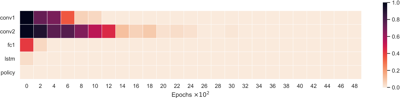
Moving on from unit ablations, we now show the re-initialisation robustness, as well as the change in - and -norms of the parameters of my trained Fetch and Jaco agents in Figures 17 and 18, respectively. We use re-initialisation robustness to study the effect of task complexity (training with and without DR, and with and without proprioceptive inputs), but with networks of similar capacity. Our results are mostly in line with Zhang et al. (Zhang et al. 2019)—despite continual changes in the weights during training (as measured by weight norms), the latter layers of the network are robust to re-initialisation after a few epochs of training, and in the case of the Fetch agents, the policy layer is robust to re-initialisation to the original set of weights. The agents trained with DR are less robust to re-initialisation during early-to-intermediate stages of training, implying that meaningful changes in the learned representations occur for longer periods within the entirety of training. In particular, the Jaco agent trained with DR and without proprioception continues to improve for a significantly longer duration than all other models.
For nearly all agents, the recurrent layer is quite robust to re-initialisation to the original set of weights (despite noticeable changes in the weights as measured by both the - -norms)—while this does not necessarily indicate that the agents do not utilise information over time, it does imply that training the recurrent connections is largely unnecessary for these tasks—a hypothesis we test further in Subsection 4.6. While the fully-connected layer benefits from training during the initial epoch across all models, it takes particularly long to train in the case of the Jaco agent trained with DR and proprioception (Figure 18j), indicating the difficulty of the task.


4.6 Recurrent Ablation
To test how useful the LSTM is, we set the hidden and cell states to constant values and re-evaluated all models. Rather than naively zeroing the hidden states, which may not be representative of the values during rollouts, we instead use the empirical average values, as calculated over the normal execution of the models in testing. Table 4 shows the results of this ablation—there is a slight effect for agents trained without DR, but a significant effect for agents trained with DR. This indicates that recurrent processing may not be necessary for solving either robotic task without DR, but it is useful when DR is active.
| Robot | DR | Prop. | Standard | Constant Hidden |
| Fetch | ✗ | ✗ | 1.000 | 0.988 |
| Fetch | ✗ | ✓ | 1.000 | 0.990 |
| Fetch | ✓ | ✗ | 0.983 | 0.658 |
| Fetch | ✓ | ✓ | 0.997 | 0.838 |
| Jaco | ✗ | ✗ | 0.995 | 0.919 |
| Jaco | ✗ | ✓ | 0.995 | 0.943 |
| Jaco | ✓ | ✗ | 0.650 | 0.422 |
| Jaco | ✓ | ✓ | 0.991 | 0.746 |
4.7 Entanglement


| Robot | DR | Prop. | 1st Conv. | 2nd Conv. | FC | LSTM |
| Fetch | ✗ | ✗ | 0.11 | 0.30 | 0.56 | 0.68 |
| Fetch | ✗ | ✓ | 0.12 | 0.30 | 0.45 | 0.45 |
| Fetch | ✓ | ✗ | 0.23 | 0.38 | 0.62 | 0.92 |
| Fetch | ✓ | ✓ | 0.24 | 0.41 | 0.58 | 1.15 |
| Jaco | ✗ | ✗ | 0.14 | 0.29 | 0.52 | 0.68 |
| Jaco | ✗ | ✓ | 0.11 | 0.08 | 0.43 | 0.66 |
| Jaco | ✓ | ✗ | 0.41 | 0.37 | 0.55 | 0.73 |
| Jaco | ✓ | ✓ | 0.65 | 0.56 | 1.21 | 1.37 |
Firstly, we consider the quantitative analysis of activations from different trained agents under the different training conditions. Table 5 contains the entanglement scores (Frosst et al. 2019) of the different trained agents, calculated across the first 4 layers (not including the policy/value outputs); as with the original work, we use a 2D t-SNE (Maaten and Hinton 2008) embedding for the activations. There are two noticeable trends. Firstly, the entanglement scores increase deeper into the network; this supports the notion that the different testing conditions can result in very different visual observations, but the difference between them diminishes as they are further processed by the networks. Secondly, the agents trained with DR have noticeably higher entanglement scores for each layer as compared to their equivalents trained without DR. This quantitatively supports the idea that DR makes agents largely invariant to nuisance visual factors (as opposed to the agents finding different strategies to cope with different visual conditions).
We can also qualitatively support these findings by visualising the same activations in 2D (Figure 19). We use three common embedding techniques in order to show different aspects of the data. Firstly, we use PCA (Pearson 1901), which linearly embeds the data into dimensions which explain the most variance in the original data; as a result, linearly separable clusters have very different global characteristics. Secondly, we use t-SNE (Maaten and Hinton 2008), which attempts to retain local structure in the data by calculating pairwise similarities between datapoints and creating a constrained graph layout in which distances in the original high-dimensional and the low-dimensional projection are preserved as much as possible. Thirdly, we use uniform manifold approximation and projection (UMAP) (McInnes et al. 2018), which operates similarly to t-SNE at a high level, but better preserves global structure. Although it is possible to tune t-SNE (Wattenberg et al. 2016), by default, UMAP better shows relevant global structure.
5 Discussion
A primary goal of these experiments was to uncover the effects of DR, through a comparison between agents trained either with or without DR. In line with prior work, DR improves performance across a wider distribution of testing conditions. In particular, our implementation of DR, which varied colours and textures, allowed generalisation to scenarios with “local” perturbations, but was more variable when more global changes were made to the setup; overall, agents trained with DR were nearly always more robust than agents trained without (Subsection 3.4). Adding DR to a task makes it more challenging to solve, in terms of sample complexity, although under the current experimental setup the models do not appear to require additional architectural depth, as all agents99 9 Except for the Jaco agent trained with DR and without proprioception, which has lower final performance under standard visuals. are robust to re-initialisation of the final (policy) layer (Subsection 4.5). The application of entanglement (Frosst et al. 2019), with respect to visual perturbations, shows that throughout the network the representations that are learned appear to be more invariant to these changes in the visuals, as the embeddings of representations from the different conditions have higher overlap (Subsection 4.7).
At the lower levels of the networks, DR results in significant changes in the -norms of the convolutional filters (Subsection 4.3), with more sophisticated feature detectors (Subsection 4.2). Supporting this, visualising the saliency maps of the agents shows that DR agents have more focused attention on task-specific features, such as the arm or ball (Subsection 4.1). Counter to initial expectations, we did not find that DR reduced the variability of performance under convolutional filter ablations—the agents merely have better baseline performance (Subsection 4.4). Deeper within the networks, we found that DR caused the agents to utilise the recurrent dynamics of the LSTM, whilst the agents trained without DR were hardly impacted by keeping their recurrent state constant (Subsection 4.6).
While we observe these general trends, it is notable that some of the results are not a priori as obvious. For example, even when provided with proprioceptive inputs, the Fetch agent trained without DR still uses its visual inputs for self-localisation (Subsection 4.1), although the addition of DR removes this observed effect. We believe that the relative simplicity of the Fetch reaching task—including both sensing and actuation—leads to less pronounced effects with DR (Subsection 3.4). The most unexpected finding was that the performance of the Jaco agent trained with DR and without proprioception dropped when shifting from DR visuals to the standard simulator visuals, demonstrating that DR can overfit (Subsection 3.3). With proprioception the gap disappears, which supports the idea that the form of input can have a significant effect on generalisation in agents (Hill et al. 2019)—meriting further investigation.
This work has focused on understanding the effects of DR, but also has a dual purpose, which is to inform research in an opposite sense: in situations where DR is expensive or even infeasible, what approaches can we take to improve generalisation in sim2real transfer? If certain characteristics are positively correlated with DR training, explicitly enforcing them—without requiring the DR pipeline—may also lead to improved generalisation. For instance, Cobbe et al. (Cobbe et al. 2018) showed that standard regularisation techniques improve generalisation to a limited extent. Similarly, Pinto et al. (Pinto et al. 2017) showed that adversarial training could improve the robustness of DRL policies. In line with this, enforcing greater spatial structure in the convolutional filters (Subsection 2.2.4), which is higher in agents trained with DR (Subsection 4.3), could be used as a novel regularisation objective.
A broader goal of these experiments was to assess the suitability of interpretability methods within the context of DRL. Beyond noticing limitations as discussed in previous works (Mahendran and Vedaldi 2015; Kindermans et al. 2016), there is a larger positive outcome from using a wide suite of interpretability techniques. Firstly, when used together they can cross-check the validity of each other’s results. For example, supposedly “dead” units in the Jaco model with DR and proprioceptive inputs do in fact worsen performance when ablated (Subsection 4.2). Additionally, although the LSTM layer within DR agents are robust to re-initialisation at early stages of training (Subsection 4.5), the recurrent ablations show that the agents depend heavily on recurrent processing (Subsection 4.6). Secondly, the complementary answers these techniques provide leads to a better understanding of the model as a whole. For instance, unit ablations (Subsection 4.4) can be related to diversity in activation maximisation (Subsection 4.2), and entanglement (Subsection 4.7) can explain the generalisation of agents trained with DR (Subsection 3.4). Given these benefits, we therefore recommend a holistic approach of interpretability techniques to be able to draw correct and informative conclusions.
References
- Andrychowicz et al. (2018) Andrychowicz, M., Baker, B., Chociej, M., Jozefowicz, R., McGrew, B., Pachocki, J., Petron, A., Plappert, M., Powell, G., Ray, A., et al., 2018. Learning dexterous in-hand manipulation. arXiv preprint arXiv:1808.00177 .
- Arulkumaran et al. (2017) Arulkumaran, K., Deisenroth, M.P., Brundage, M., Bharath, A.A., 2017. Deep reinforcement learning: A brief survey. IEEE Signal Processing Magazine 34, 26–38.
- Aubry and Russell (2015) Aubry, M., Russell, B.C., 2015. Understanding deep features with computer-generated imagery, in: International Conference on Computer Vision, pp. 2875–2883.
- Bach et al. (2015) Bach, S., Binder, A., Montavon, G., Klauschen, F., Müller, K.R., Samek, W., 2015. On pixel-wise explanations for non-linear classifier decisions by layer-wise relevance propagation. PloS one 10, e0130140.
- Barto et al. (1983) Barto, A.G., Sutton, R.S., Anderson, C.W., 1983. Neuronlike adaptive elements that can solve difficult learning control problems. IEEE Transactions on Systems, Man, and Cybernetics , 834–846.
- Bellido and Fiesler (1993) Bellido, I., Fiesler, E., 1993. Do backpropagation trained neural networks have normal weight distributions?, in: International Conference on Artificial Neural Networks, Springer. pp. 772–775.
- Bousmalis et al. (2018) Bousmalis, K., Irpan, A., Wohlhart, P., Bai, Y., Kelcey, M., Kalakrishnan, M., Downs, L., Ibarz, J., Pastor, P., Konolige, K., et al., 2018. Using simulation and domain adaptation to improve efficiency of deep robotic grasping, in: International Conference on Robotics and Automation, IEEE. pp. 4243–4250.
- Brockman et al. (2016) Brockman, G., Cheung, V., Pettersson, L., Schneider, J., Schulman, J., Tang, J., Zaremba, W., 2016. OpenAI Gym. arXiv preprint arXiv:1606.01540 .
- Chebotar et al. (2018) Chebotar, Y., Handa, A., Makoviychuk, V., Macklin, M., Issac, J., Ratliff, N., Fox, D., 2018. Closing the sim-to-real loop: Adapting simulation randomization with real world experience. arXiv preprint arXiv:1810.05687 .
- Cobbe et al. (2018) Cobbe, K., Klimov, O., Hesse, C., Kim, T., Schulman, J., 2018. Quantifying generalization in reinforcement learning. arXiv preprint arXiv:1812.02341 .
- Craven and Shavlik (1996) Craven, M., Shavlik, J.W., 1996. Extracting tree-structured representations of trained networks, in: Advances in Neural Information Processing Systems, pp. 24–30.
- Deisenroth et al. (2013) Deisenroth, M.P., Neumann, G., Peters, J., et al., 2013. A survey on policy search for robotics. Foundations and Trends® in Robotics 2, 1–142.
- Donahue et al. (2014) Donahue, J., Jia, Y., Vinyals, O., Hoffman, J., Zhang, N., Tzeng, E., Darrell, T., 2014. Decaf: A deep convolutional activation feature for generic visual recognition, in: International Conference on Machine Learning, pp. 647–655.
- Doshi-Velez and Kim (2017) Doshi-Velez, F., Kim, B., 2017. Towards a rigorous science of interpretable machine learning. arXiv preprint arXiv:1702.08608 .
- Elman (1989) Elman, J.L., 1989. Representation and structure in connectionist models. Technical Report. Univ. of California at San Diego, La Jolla Center For Research In Language.
- Erhan et al. (2009) Erhan, D., Bengio, Y., Courville, A., Vincent, P., 2009. Visualizing higher-layer features of a deep network. Technical Report 1341. University of Montreal.
- François-Lavet et al. (2018) François-Lavet, V., Henderson, P., Islam, R., Bellemare, M.G., Pineau, J., et al., 2018. An introduction to deep reinforcement learning. Foundations and Trends® in Machine Learning 11, 219–354.
- Freitas (2014) Freitas, A.A., 2014. Comprehensible classification models: a position paper. Explorations Newsletter 15, 1–10.
- Frosst et al. (2019) Frosst, N., Papernot, N., Hinton, G., 2019. Analyzing and improving representations with the soft nearest neighbor loss, in: International Conference on Machine Learning, pp. 2012–2020.
- Gers et al. (2000) Gers, F.A., Schmidhuber, J., Cummins, F., 2000. Learning to forget: Continual prediction with lstm. Neural Computation 12, 2451–2471.
- Girshick et al. (2014) Girshick, R., Donahue, J., Darrell, T., Malik, J., 2014. Rich feature hierarchies for accurate object detection and semantic segmentation, in: Conference on Computer Vision and Pattern Recognition, pp. 580–587.
- Glorot and Bengio (2010) Glorot, X., Bengio, Y., 2010. Understanding the difficulty of training deep feedforward neural networks, in: International Conference on Artificial Intelligence and Statistics, pp. 249–256.
- Greydanus et al. (2018) Greydanus, S., Koul, A., Dodge, J., Fern, A., 2018. Visualizing and understanding atari agents, in: International Conference on Machine Learning, pp. 1787–1796.
- Gu et al. (2017) Gu, S., Holly, E., Lillicrap, T., Levine, S., 2017. Deep reinforcement learning for robotic manipulation with asynchronous off-policy updates, in: International Conference on Robotics and Automation, IEEE. pp. 3389–3396.
- Guidotti et al. (2018) Guidotti, R., Monreale, A., Ruggieri, S., Turini, F., Giannotti, F., Pedreschi, D., 2018. A survey of methods for explaining black box models. ACM Computing Surveys 51, 93.
- Hamel and Eck (2010) Hamel, P., Eck, D., 2010. Learning features from music audio with deep belief networks., in: ISMIR, Utrecht, The Netherlands. pp. 339–344.
- Han et al. (2015) Han, S., Pool, J., Tran, J., Dally, W., 2015. Learning both weights and connections for efficient neural network, in: Advances in Neural Information Processing Systems, pp. 1135–1143.
- Hansen and Salamon (1990) Hansen, L.K., Salamon, P., 1990. Neural network ensembles. IEEE Transactions on Pattern Analysis & Machine Intelligence , 993–1001.
- Hanson and Burr (1990) Hanson, S.J., Burr, D.J., 1990. What connectionist models learn: Learning and representation in connectionist networks. Behavioral and Brain Sciences 13, 471–489.
- Hanson and Pratt (1989) Hanson, S.J., Pratt, L.Y., 1989. Comparing biases for minimal network construction with back-propagation, in: Advances in Neural Information Processing Systems, pp. 177–185.
- Hassibi and Stork (1993) Hassibi, B., Stork, D.G., 1993. Second order derivatives for network pruning: Optimal brain surgeon, in: Advances in Neural Information Processing Systems, pp. 164–171.
- He et al. (2015) He, K., Zhang, X., Ren, S., Sun, J., 2015. Delving deep into rectifiers: Surpassing human-level performance on imagenet classification, in: International Conference on Computer Vision, pp. 1026–1034.
- Hill et al. (2019) Hill, F., Lampinen, A., Schneider, R., Clark, S., Botvinick, M., McClelland, J.L., Santoro, A., 2019. Emergent systematic generalization in a situated agent. arXiv preprint arXiv:1910.00571 .
- Hinton and Shallice (1991) Hinton, G.E., Shallice, T., 1991. Lesioning an attractor network: Investigations of acquired dyslexia. Psychological review 98, 74.
- Hochreiter and Schmidhuber (1997) Hochreiter, S., Schmidhuber, J., 1997. Long short-term memory. Neural Computation 9, 1735–1780.
- Ilyas et al. (2018) Ilyas, A., Engstrom, L., Santurkar, S., Tsipras, D., Janoos, F., Rudolph, L., Madry, A., 2018. Are deep policy gradient algorithms truly policy gradient algorithms? arXiv preprint arXiv:1811.02553 .
- Jakobi et al. (1995) Jakobi, N., Husbands, P., Harvey, I., 1995. Noise and the reality gap: The use of simulation in evolutionary robotics, in: European Conference on Artificial Life, Springer. pp. 704–720.
- James et al. (2017) James, S., Davison, A.J., Johns, E., 2017. Transferring end-to-end visuomotor control from simulation to real world for a multi-stage task, in: Conference on Robot Learning, pp. 334–343.
- Justesen et al. (2018) Justesen, N., Torrado, R.R., Bontrager, P., Khalifa, A., Togelius, J., Risi, S., 2018. Procedural level generation improves generality of deep reinforcement learning. arXiv preprint arXiv:1806.10729 .
- Khabou et al. (1999) Khabou, M.A., Gader, P.D., Shi, H., 1999. Entropy optimized morphological shared-weight neural networks. Optical Engineering 38, 263–274.
- Kindermans et al. (2017) Kindermans, P.J., Hooker, S., Adebayo, J., Alber, M., Schütt, K.T., Dähne, S., Erhan, D., Kim, B., 2017. The (un) reliability of saliency methods, in: NeurIPS Interpreting, Explaining and Visualizing Deep Learning Workshop.
- Kindermans et al. (2016) Kindermans, P.J., Schütt, K., Müller, K.R., Dähne, S., 2016. Investigating the influence of noise and distractors on the interpretation of neural networks, in: NeurIPS Interpretable Machine Learning in Complex Systems Workshop.
- Kingma and Ba (2014) Kingma, D.P., Ba, J., 2014. Adam: A method for stochastic optimization. arXiv preprint arXiv:1412.6980 .
- Kragic and Vincze (2009) Kragic, D., Vincze, M., 2009. Vision for robotics. Foundations and Trends in Robotics 1, 1–78.
- Krizhevsky et al. (2012) Krizhevsky, A., Sutskever, I., Hinton, G.E., 2012. Imagenet classification with deep convolutional neural networks, in: Advances in Neural Information Processing Systems, pp. 1097–1105.
- Krkic et al. (1996) Krkic, M., Roberts, S.J., Rezek, I., Jordan, C., 1996. Eeg-based assessment of anaesthetic depth using neural networks .
- Lapuschkin et al. (2019) Lapuschkin, S., Wäldchen, S., Binder, A., Montavon, G., Samek, W., Müller, K.R., 2019. Unmasking clever hans predictors and assessing what machines really learn. Nature Communications 10, 1096.
- LeCun et al. (1998) LeCun, Y., Bottou, L., Orr, G.B., Müller, K.R., 1998. Efficient backprop, in: Neural Networks: Tricks of the Trade. Springer, pp. 9–50.
- LeCun et al. (1990) LeCun, Y., Denker, J.S., Solla, S.A., 1990. Optimal brain damage, in: Advances in Neural Information Processing Systems, pp. 598–605.
- Levine et al. (2016) Levine, S., Finn, C., Darrell, T., Abbeel, P., 2016. End-to-end training of deep visuomotor policies. The Journal of Machine Learning Research 17, 1334–1373.
- Levine et al. (2018) Levine, S., Pastor, P., Krizhevsky, A., Ibarz, J., Quillen, D., 2018. Learning hand-eye coordination for robotic grasping with deep learning and large-scale data collection. The International Journal of Robotics Research 37, 421–436.
- Li et al. (2017) Li, H., Kadav, A., Durdanovic, I., Samet, H., Graf, H.P., 2017. Pruning filters for efficient convnets, in: International Conference on Learning Representations.
- Lin et al. (2013) Lin, M., Chen, Q., Yan, S., 2013. Network in network. International Conference on Learning Representations .
- Liu et al. (2018) Liu, Z., Xu, J., Peng, X., Xiong, R., 2018. Frequency-domain dynamic pruning for convolutional neural networks, in: Advances in Neural Information Processing Systems, pp. 1043–1053.
- Lundberg and Lee (2017) Lundberg, S.M., Lee, S.I., 2017. A unified approach to interpreting model predictions, in: Advances in Neural Information Processing Systems, pp. 4765–4774.
- Luo and Wu (2017) Luo, J.H., Wu, J., 2017. An entropy-based pruning method for cnn compression. arXiv preprint arXiv:1706.05791 .
- Maaten and Hinton (2008) Maaten, L.v.d., Hinton, G., 2008. Visualizing data using t-sne. Journal of machine learning research 9, 2579–2605.
- Madry et al. (2018) Madry, A., Makelov, A., Schmidt, L., Tsipras, D., Vladu, A., 2018. Towards deep learning models resistant to adversarial attacks, in: International Conference on Learning Representations.
- Mahendran and Vedaldi (2015) Mahendran, A., Vedaldi, A., 2015. Understanding deep image representations by inverting them, in: Conference on Computer Vision and Pattern Recognition, pp. 5188–5196.
- Martinez-Gomez et al. (2014) Martinez-Gomez, J., Fernandez-Caballero, A., Garcia-Varea, I., Rodriguez, L., Romero-Gonzalez, C., 2014. A taxonomy of vision systems for ground mobile robots. International Journal of Advanced Robotic Systems 11, 111.
- McInnes et al. (2018) McInnes, L., Healy, J., Melville, J., 2018. Umap: Uniform manifold approximation and projection for dimension reduction. arXiv preprint arXiv:1802.03426 .
- Misra et al. (2004) Misra, H., Ikbal, S., Bourlard, H., Hermansky, H., 2004. Spectral entropy based feature for robust asr, in: International Conference on Acoustics, Speech, and Signal Processing, IEEE. pp. I–193.
- Mnih et al. (2016) Mnih, V., Badia, A.P., Mirza, M., Graves, A., Lillicrap, T., Harley, T., Silver, D., Kavukcuoglu, K., 2016. Asynchronous methods for deep reinforcement learning, in: International Conference on Machine Learning, pp. 1928–1937.
- Mnih et al. (2015) Mnih, V., Kavukcuoglu, K., Silver, D., Rusu, A.A., Veness, J., Bellemare, M.G., Graves, A., Riedmiller, M., Fidjeland, A.K., Ostrovski, G., et al., 2015. Human-level control through deep reinforcement learning. Nature 518, 529.
- Mohamed et al. (2012) Mohamed, A.r., Hinton, G., Penn, G., 2012. Understanding how deep belief networks perform acoustic modelling. Neural Networks , 6–9.
- Morch et al. (1995) Morch, N., Kjems, U., Hansen, L.K., Svarer, C., Law, I., Lautrup, B., Strother, S., Rehm, K., 1995. Visualization of neural networks using saliency maps, in: International Conference on Neural Networks, IEEE. pp. 2085–2090.
- Mordvintsev et al. (2015) Mordvintsev, A., Olah, C., Tyka, M., 2015. Inceptionism: Going deeper into neural networks .
- Nair and Hinton (2010) Nair, V., Hinton, G.E., 2010. Rectified linear units improve restricted boltzmann machines, in: International Conference on Machine Learning, pp. 807–814.
- Nguyen et al. (2015) Nguyen, A., Yosinski, J., Clune, J., 2015. Deep neural networks are easily fooled: High confidence predictions for unrecognizable images, in: Conference on Computer Vision and Pattern Recognition, pp. 427–436.
- Odena et al. (2016) Odena, A., Dumoulin, V., Olah, C., 2016. Deconvolution and checkerboard artifacts. Distill URL: http://distill.pub/2016/deconv-checkerboard, doi:10.23915/distill.00003.
- Olah et al. (2017) Olah, C., Mordvintsev, A., Schubert, L., 2017. Feature visualization. Distill doi:10.23915/distill.00007. https://distill.pub/2017/feature-visualization.
- Packer et al. (2018) Packer, C., Gao, K., Kos, J., Krähenbühl, P., Koltun, V., Song, D., 2018. Assessing generalization in deep reinforcement learning. arXiv preprint arXiv:1810.12282 .
- Pascanu et al. (2013) Pascanu, R., Mikolov, T., Bengio, Y., 2013. On the difficulty of training recurrent neural networks, in: International Conference on Machine Learning, pp. 1310–1318.
- Paszke et al. (2017) Paszke, A., Gross, S., Chintala, S., Chanan, G., Yang, E., DeVito, Z., Lin, Z., Desmaison, A., Antiga, L., Lerer, A., 2017. Automatic differentiation in pytorch .
- Pearson (1901) Pearson, K., 1901. Liii. on lines and planes of closest fit to systems of points in space. The London, Edinburgh, and Dublin Philosophical Magazine and Journal of Science 2, 559–572.
- Peng et al. (2018) Peng, X.B., Andrychowicz, M., Zaremba, W., Abbeel, P., 2018. Sim-to-real transfer of robotic control with dynamics randomization, in: International Conference on Robotics and Automation, IEEE. pp. 1–8.
- Pinto et al. (2017) Pinto, L., Davidson, J., Sukthankar, R., Gupta, A., 2017. Robust adversarial reinforcement learning, in: International Conference on Machine Learning, pp. 2817–2826.
- Plappert et al. (2018) Plappert, M., Andrychowicz, M., Ray, A., McGrew, B., Baker, B., Powell, G., Schneider, J., Tobin, J., Chociej, M., Welinder, P., et al., 2018. Multi-goal reinforcement learning: Challenging robotics environments and request for research. arXiv preprint arXiv:1802.09464 .
- Rauber et al. (2017) Rauber, P.E., Fadel, S.G., Falcao, A.X., Telea, A.C., 2017. Visualizing the hidden activity of artificial neural networks. IEEE Transactions on Visualization and Computer Graphics 23, 101–110.
- Reed (1993) Reed, R., 1993. Pruning algorithms-a survey. IEEE Transactions on Neural Networks 4, 740–747.
- Ribeiro et al. (2016) Ribeiro, M.T., Singh, S., Guestrin, C., 2016. Why should i trust you?: Explaining the predictions of any classifier, in: International Conference on Knowledge Discovery and Data Mining, ACM. pp. 1135–1144.
- Rusu et al. (2017) Rusu, A.A., Večerík, M., Rothörl, T., Heess, N., Pascanu, R., Hadsell, R., 2017. Sim-to-real robot learning from pixels with progressive nets, in: Conference on Robot Learning, pp. 262–270.
- Sadeghi and Levine (2017) Sadeghi, F., Levine, S., 2017. Cad2rl: Real single-image flight without a single real image, in: Robotics: Science and Systems.
- Salakhutdinov and Hinton (2007) Salakhutdinov, R., Hinton, G., 2007. Learning a nonlinear embedding by preserving class neighbourhood structure, in: Artificial Intelligence and Statistics, pp. 412–419.
- Saxe et al. (2014) Saxe, A.M., McClelland, J.L., Ganguli, S., 2014. Exact solutions to the nonlinear dynamics of learning in deep linear neural networks, in: International Conference on Learning Representations.
- Schulman et al. (2015) Schulman, J., Moritz, P., Levine, S., Jordan, M., Abbeel, P., 2015. High-dimensional continuous control using generalized advantage estimation. arXiv preprint arXiv:1506.02438 .
- Schulman et al. (2017) Schulman, J., Wolski, F., Dhariwal, P., Radford, A., Klimov, O., 2017. Proximal policy optimization algorithms. arXiv preprint arXiv:1707.06347 .
- Selvaraju et al. (2017) Selvaraju, R.R., Cogswell, M., Das, A., Vedantam, R., Parikh, D., Batra, D., 2017. Grad-cam: Visual explanations from deep networks via gradient-based localization, in: International Conference on Computer Vision, pp. 618–626.
- Shrikumar et al. (2017) Shrikumar, A., Greenside, P., Kundaje, A., 2017. Learning important features through propagating activation differences, in: International Conference on Machine Learning, JMLR. org. pp. 3145–3153.
- Sietsma and Dow (1988) Sietsma, J., Dow, R.J., 1988. Neural net pruning - why and how, in: International Conference on Neural Networks, pp. 325–333.
- Sietsma and Dow (1991) Sietsma, J., Dow, R.J., 1991. Creating artificial neural networks that generalize. Neural Networks 4, 67–79.
- Simonyan et al. (2013) Simonyan, K., Vedaldi, A., Zisserman, A., 2013. Deep inside convolutional networks: Visualising image classification models and saliency maps. arXiv preprint arXiv:1312.6034 .
- Springenberg et al. (2015) Springenberg, J., Dosovitskiy, A., Brox, T., Riedmiller, M., 2015. Striving for simplicity: The all convolutional net, in: International Conference on Learning Representations (Workshop Track).
- Srinivasan et al. (2005) Srinivasan, V., Eswaran, C., Sriraam, N, 2005. Artificial neural network based epileptic detection using time-domain and frequency-domain features. Journal of Medical Systems 29, 647–660.
- Sturmfels et al. (2020) Sturmfels, P., Lundberg, S., Lee, S.I., 2020. Visualizing the impact of feature attribution baselines. Distill 5, e21.
- Such et al. (2018) Such, F., Madhavan, V., Liu, R., Wang, R., Castro, P., Li, Y., Schubert, L., Bellemare, M.G., Clune, J., Lehman, J., 2018. An atari model zoo for analyzing, visualizing, and comparing deep reinforcement learning agents, in: NeurIPS Deep RL Workshop.
- Sundararajan et al. (2017) Sundararajan, M., Taly, A., Yan, Q., 2017. Axiomatic attribution for deep networks, in: International Conference on Machine Learning, JMLR. org. pp. 3319–3328.
- Sutton and Barto (2018) Sutton, R.S., Barto, A.G., 2018. Reinforcement learning: An introduction. MIT press.
- Tobin et al. (2017) Tobin, J., Fong, R., Ray, A., Schneider, J., Zaremba, W., Abbeel, P., 2017. Domain randomization for transferring deep neural networks from simulation to the real world, in: International Conference on Intelligent Robots and Systems, IEEE. pp. 23–30.
- Todorov et al. (2012) Todorov, E., Erez, T., Tassa, Y., 2012. Mujoco: A physics engine for model-based control, in: International Conference on Intelligent Robots and Systems, IEEE. pp. 5026–5033.
- Tzeng et al. (2015) Tzeng, E., Devin, C., Hoffman, J., Finn, C., Peng, X., Levine, S., Saenko, K., Darrell, T., 2015. Towards adapting deep visuomotor representations from simulated to real environments. arXiv preprint arXiv:1511.07111 2.
- Uesato et al. (2018) Uesato, J., Kumar, A., Szepesvari, C., Erez, T., Ruderman, A., Anderson, K., Heess, N., Kohli, P., et al., 2018. Rigorous agent evaluation: An adversarial approach to uncover catastrophic failures. arXiv preprint arXiv:1812.01647 .
- Wattenberg et al. (2016) Wattenberg, M., Viégas, F., Johnson, I., 2016. How to use t-sne effectively. Distill 1, e2.
- Wierstra et al. (2007) Wierstra, D., Foerster, A., Peters, J., Schmidhuber, J., 2007. Solving deep memory pomdps with recurrent policy gradients, in: International Conference on Artificial Neural Networks, Springer. pp. 697–706.
- Williams and Peng (1991) Williams, R.J., Peng, J., 1991. Function optimization using connectionist reinforcement learning algorithms. Connection Science 3, 241–268.
- Witty et al. (2018) Witty, S., Lee, J.K., Tosch, E., Atrey, A., Littman, M., Jensen, D., 2018. Measuring and characterizing generalization in deep reinforcement learning. arXiv preprint arXiv:1812.02868 .
- Yamins and DiCarlo (2016) Yamins, D.L., DiCarlo, J.J., 2016. Using goal-driven deep learning models to understand sensory cortex. Nature Neuroscience 19, 356.
- Zeiler and Fergus (2014) Zeiler, M.D., Fergus, R., 2014. Visualizing and understanding convolutional networks, in: European Conference on Computer Vision, Springer. pp. 818–833.
- Zhang et al. (2018a) Zhang, A., Ballas, N., Pineau, J., 2018a. A dissection of overfitting and generalization in continuous reinforcement learning. arXiv preprint arXiv:1806.07937 .
- Zhang et al. (2019) Zhang, C., Bengio, S., Singer, Y., 2019. Are all layers created equal? arXiv preprint arXiv:1902.01996 .
- Zhang et al. (2018b) Zhang, C., Vinyals, O., Munos, R., Bengio, S., 2018b. A study on overfitting in deep reinforcement learning. arXiv preprint arXiv:1804.06893 .
- Zhao et al. (2019) Zhao, C., Siguad, O., Stulp, F., Hospedales, T.M., 2019. Investigating generalisation in continuous deep reinforcement learning. arXiv preprint arXiv:1902.07015 .
- Zheng et al. (1996) Zheng, B., Qian, W., Clarke, L.P., 1996. Digital mammography: mixed feature neural network with spectral entropy decision for detection of microcalcifications. IEEE Transactions on Medical Imaging 15, 589–597.
- Zhou et al. (2016) Zhou, B., Khosla, A., Lapedriza, A., Oliva, A., Torralba, A., 2016. Learning deep features for discriminative localization, in: Conference on Computer Vision and Pattern Recognition, pp. 2921–2929.
- Zhu et al. (2017) Zhu, Y., Mottaghi, R., Kolve, E., Lim, J.J., Gupta, A., Fei-Fei, L., Farhadi, A., 2017. Target-driven visual navigation in indoor scenes using deep reinforcement learning, in: International Conference on Robotics and Automation, IEEE. pp. 3357–3364.