跳到论文正文
W Papers独立论文阅读器 arXiv:1912.08022 论文正文 计算阅读时间 · 0%
引用这篇论文根据当前论文元数据生成,正式投稿前建议核对。


License: arXiv.org perpetual non-exclusive license
arXiv:1912.08022v1 [math.NA] 17 Dec 2019

Numerical Studies of a Hemivariational Inequality for a Viscoelastic Contact Problem with Damage

Weimin Han11 1 Program in Applied Mathematical and Computational Sciences (AMCS) & Department of Mathematics, University of Iowa, Iowa City, IA 52242, USA. Email: weimin-han@uiowa.edu, Michal Jureczka22 2 Jagiellonian University in Krakow, Faculty of Mathematics and Computer Science, Lojasiewicza 6, 30-348 Krakow, Poland. Email: michal.jureczka@uj.edu.pl and  Anna Ochal33 3 Jagiellonian University in Krakow, Faculty of Mathematics and Computer Science, Lojasiewicza 6, 30-348 Krakow, Poland. Email: ochal@ii.uj.edu.pl

Abstract. This paper is devoted to the study of a hemivariational inequality modeling the quasistatic bilateral frictional contact between a viscoelastic body and a rigid foundation. The damage effect is built into the model through a parabolic differential inclusion for the damage function. A solution existence and uniqueness result is presented. A fully discrete scheme is introduced with the time derivative of the damage function approximated by the backward finite different and the spatial derivatives approximated by finite elements. An optimal order error estimate is derived for the fully discrete scheme when linear elements are used for the velocity and displacement variables, and piecewise constants are used for the damage function. Simulation results on numerical examples are reported illustrating the performance of the fully discrete scheme and the theoretically predicted convergence orders.

Keywords. Quasistatic contact, viscoelastic material, damage, hemivariational inequality, fully discrete scheme, convergence, optimal order error estimate.

Mathematical Subject Classification (2010). 65N30, 65M06, 47J20, 74M10, 74M15.

1 Introduction

In this paper, we study a mathematical model in the form of a hemivariational inequality for a quasistatic bilateral frictional contact problem between a viscoelastic body and a rigid foundation. The friction law is given in the form of subdifferential condition. Damage of the material is incorporated. Modeling, variational analysis and numerical solution of contact problems have been studied extensively; in this regard, a few comprehensive references are [22, 21, 16, 27] in the context of variational inequalities (VIs), and [23, 28] in the context of hemivariational inequalities (HVIs).

The notion of hemivariational inequalities (HVIs) was introduced in early 1980s to model mechanical problems involving non-smooth, non-monotone or multi-valued relations ([25]). Early results on modeling, mathematical analysis and engineering applications of HVIs are summarized in [26, 24]; recent summarized accounts include [4, 23, 28]. Since there are no solution formulas for HVIs in applications, numerical simulation is the only feasible approach to solving HVIs. Detailed discussion of the finite element method for solving HVIs can be found in [20]. More recently, there has been substantial progress in numerical analysis of HVIs, especially on optimal order error estimates for numerical solutions of HVIs, starting with the paper [14], followed by a sequence of papers, e.g., [2, 18, 13, 19]; the reader is referred to [17] for a recent survey.

Many contact processes are accompanied with material damage. In applications, it is very important to consider the damage effect. General mathematical models for damage were derived in [10, 11]; see also [9]. In [15], a quasistatic contact problem for a viscoelastic material is studied variationally and numerically, where the damage effect of the viscoelastic material is taken into account. Systematic variational analysis and numerical analysis of contact problems with damage effect is summarized in [27]. The mathematical problems investigated in these references are in the form of VIs. For studies of contact problems with damage in the form of HVIs, the reader is referred to [12].

This is the first paper devoted to numerical analysis of an HVI arising in a contact problem with damage. The rest of the paper is organized as follows. In Section 2, we introduce the contact problem, present its weak formulation as an HVI and comment on the solution existence and uniqueness. In Section 3, we consider a fully discrete numerical scheme for the contact problem and derive an optimal order error estimate under appropriate solution regularity assumptions. In Section 4, we report computer simulation results on a numerical example and illustrate numerical convergence orders that match the theoretical error bound.

2 The contact problem

We first introduce the pointwise formulation of the quasistatic contact problem for the contact between a viscoelastic body and a rigid foundation. The initial configuration of the body is Ω\Omega, a Lipschitz bounded domain in ℝd\mathbb{R}^{d} (d≤3d\leq 3 in applications). The body is subject to the action of volume forces of a total density 𝒇0\mbox{\boldmath{$f$}}_{0}. The boundary Γ\Gamma of the domain Ω\Omega is split into three disjoint measurable parts, Γ=Γ1∪Γ2∪Γ3\Gamma=\Gamma_{1}\cup\Gamma_{2}\cup\Gamma_{3} such that Γ1\Gamma_{1} is non-trivial. We will assume the body is fixed along Γ1\Gamma_{1}, is subject to the action of surface tractions with a total density 𝒇2\mbox{\boldmath{$f$}}_{2}. Along the contact boundary Γ3\Gamma_{3}, the body and the foundation are in bilateral contact and the frictional process is described by a generalized subdifferential inclusion.

Following [8, 16], we consider a viscoelastic constitutive law with the damage effect in the form

𝝈=𝒜​𝜺​(𝒖˙)+ℬ⁡(𝜺⁡(𝒖),ζ),\mbox{\boldmath{$\sigma$}}={\cal A}\mbox{\boldmath{$\varepsilon$}}(\dot{\mbox{\boldmath{$u$}}})+{\cal B}(\mbox{\boldmath{$\varepsilon$}}(\mbox{\boldmath{$u$}}),\zeta),

where 𝒖u is the displacement field, ζ\zeta is the damage function, 𝝈\sigma is the stress field, 𝒜{\cal A} and ℬ{\cal B} are the viscosity operator and the elasticity operator. These operators are allowed to depend on the spatial location. For convenience, we use the shorthand notation 𝒜​𝜺​(𝒖˙){\cal A}\mbox{\boldmath{$\varepsilon$}}(\dot{\mbox{\boldmath{$u$}}}) and ℬ⁡(𝜺⁡(𝒖),ζ){\cal B}(\mbox{\boldmath{$\varepsilon$}}(\mbox{\boldmath{$u$}}),\zeta) for 𝒜⁡(𝒙,𝜺⁡(𝒖˙)){\cal A}(\mbox{\boldmath{$x$}},\mbox{\boldmath{$\varepsilon$}}(\dot{\mbox{\boldmath{$u$}}})) and ℬ⁡(𝒙,𝜺⁡(𝒖),ζ){\cal B}(\mbox{\boldmath{$x$}},\mbox{\boldmath{$\varepsilon$}}(\mbox{\boldmath{$u$}}),\zeta), respectively. The symbol 𝒖˙\dot{\mbox{\boldmath{$u$}}} denotes the time derivative of 𝒖u. The time interval of interest is [0,T][0,T] for some T>0T>0.

The notion of the damage function was introduced in [10, 11] to quantify the damage to the material. It is defined to be the ratio between the elastic modulus of the damaged material and that of the original material. The value of the damage function ζ\zeta lies in [0,1][0,1]. The value ζ=1\zeta=1 indicates that there is no damage in the material, whereas the value ζ=0\zeta=0 corresponds to a completely damaged material. When 0<ζ<10<\zeta<1, there is a partial damage and the system has a reduced load carrying capacity. A popular model for the evolution of the damage function is given by a parabolic differential inclusion:

ζ˙−κ​△​ζ+∂I[0,1]​(ζ)∋ϕ⁡(𝜺⁡(𝒖),ζ),\dot{\zeta}-\kappa\,\triangle\zeta+\partial I_{[0,1]}(\zeta)\ni\phi(\mbox{\boldmath{$\varepsilon$}}(\mbox{\boldmath{$u$}}),\zeta),

where κ>0\kappa>0 is a constant microcrack diffusion coefficient, I[0,1]I_{[0,1]} is the indicator function of the interval [0,1][0,1], ∂I[0,1]\partial I_{[0,1]} is the convex subdifferential of I[0,1]I_{[0,1]}, and ϕ\phi is the mechanical source of damage, depending on the strain and the damage itself. On the boundary Γ\Gamma, a homogeneous Neumann condition is described for ζ\zeta.

For a vector 𝒗v defined on Γ\Gamma, we let vν=𝒗⋅𝝂v_{\nu}=\mbox{\boldmath{$v$}}\cdot\mbox{\boldmath{$\nu$}} be its normal component, and let 𝒗τ=𝒗−vν​𝝂\mbox{\boldmath{$v$}}_{\tau}=\mbox{\boldmath{$v$}}-v_{\nu}\mbox{\boldmath{$\nu$}} be its tangential component. For a stress tensor 𝝈\sigma defined on Γ\Gamma, we let σν=(𝝈𝝂)⋅𝝂\sigma_{\nu}=(\mbox{\boldmath{$\sigma$}}\mbox{\boldmath{$\nu$}})\cdot\mbox{\boldmath{$\nu$}} and 𝝈τ=𝝈𝝂−σν​𝝂\mbox{\boldmath{$\sigma$}}_{\tau}=\mbox{\boldmath{$\sigma$}}\mbox{\boldmath{$\nu$}}-\sigma_{\nu}\mbox{\boldmath{$\nu$}} be its normal and tangential components, respectively.

Denote by 𝒖0\mbox{\boldmath{$u$}}_{0} and ζ0\zeta_{0} the initial values of the displacement and the damage function. The pointwise formulation of the contact problem is as follows.

Problem 2.1

Find a displacement field 𝐮:Ω×[0,T]→ℝd\mbox{\boldmath{$u$}}:\Omega\times[0,T]\to\mathbb{R}^{d}, a stress field 𝛔:Ω×[0,T]→𝕊d\mbox{\boldmath{$\sigma$}}:\Omega\times[0,T]\to\mathbb{S}^{d}, and a damage field ζ:Ω×[0,T]→ℝ\zeta:\Omega\times[0,T]\to\mathbb{R} such that

𝛔\sigma =𝒜​𝜺​(𝒖˙)+ℬ⁡(𝜺⁡(𝒖),ζ)\displaystyle={\cal A}\mbox{\boldmath{$\varepsilon$}}(\dot{\mbox{\boldmath{$u$}}})+{\cal B}(\mbox{\boldmath{$\varepsilon$}}(\mbox{\boldmath{$u$}}),\zeta) in​Ω×(0,T),\displaystyle{\rm in}\ \Omega\times(0,T), (2.1)
ζ˙−κ​△​ζ+∂I[0,1]​(ζ)\displaystyle\dot{\zeta}-\kappa\,\triangle\zeta+\partial I_{[0,1]}(\zeta) ∋ϕ⁡(𝜺⁡(𝒖),ζ)\displaystyle\ni\phi(\mbox{\boldmath{$\varepsilon$}}(\mbox{\boldmath{$u$}}),\zeta) in​Ω×(0,T),\displaystyle{\rm in}\ \Omega\times(0,T), (2.2)
Div​𝝈+𝒇0\displaystyle{\rm Div}\,\mbox{\boldmath{$\sigma$}}+{\mbox{\boldmath{$f$}}}_{0} =𝟎\displaystyle=\mbox{\boldmath{$0$}} in​Ω×(0,T),\displaystyle{\rm in}\ \Omega\times(0,T), (2.3)
∂ζ∂ν\displaystyle\frac{\partial\zeta}{\partial\nu} =0\displaystyle=0 on​Γ×(0,T),\displaystyle{\rm on}\ \Gamma\times(0,T), (2.4)
𝐮u =𝟎\displaystyle=\mbox{\boldmath{$0$}} on​Γ1×(0,T),\displaystyle{\rm on}\ \Gamma_{1}\times(0,T), (2.5)
𝛔\sigma𝛎\nu =𝒇2\displaystyle={\mbox{\boldmath{$f$}}}_{2} on​Γ2×(0,T),\displaystyle{\rm on}\ \Gamma_{2}\times(0,T), (2.6)
uν\displaystyle u_{\nu} =0,−𝝈τ∈∂j⁡(𝒖˙τ)\displaystyle=0,\ -\mbox{\boldmath{$\sigma$}}_{\tau}\in\partial j(\dot{\mbox{\boldmath{$u$}}}_{\tau}) on​Γ3×(0,T),\displaystyle{\rm on}\ \Gamma_{3}\times(0,T), (2.7)
𝒖⁡(0)\displaystyle\mbox{\boldmath{$u$}}(0) =𝒖0,ζ⁡(0)=ζ0\displaystyle=\mbox{\boldmath{$u$}}_{0},\ \zeta(0)=\zeta_{0} in​Ω.\displaystyle{\rm in}\ \Omega. (2.8)

We already know that (2.1) is the viscoelastic constitutive law with damage, and (2.2) is the evolution relation for the damage function. We consider a quasistatic contact process and (2.3) is the corresponding equilibrium equation. The initial conditions for the displacement field and the damage function are given by (2.8). The relations (2.4)–(2.7) are the boundary condition for the damage function, the displacement boundary condition on Γ1\Gamma_{1}, the traction boundary condition on Γ2\Gamma_{2}, and the bilateral friction contact condition on Γ3\Gamma_{3}. Here, the friction dissipation pseudopotential jj will be assumed to be Lipschitz continuous, and ∂j\partial j represents the generalized subdifferential in the sense of Clarke (cf. [6, 7]). We will also need the notion of the generalized directional derivative in the sense of Clarke. Let VV be a Banach space and let ψ:V→ℝ\psi\colon V\to\mathbb{R} be a locally Lipschitz continuous functional. Recall that the generalized directional derivative of ψ\psi at u∈Vu\in V in the direction v∈Vv\in V is

ψ0​(u,v):=lim supw→u,λ↓0ψ⁡(w+λ​v)−ψ⁡(w)λ,\psi^{0}(u;v):=\limsup_{w\to u,\,\lambda\downarrow 0}\frac{\psi(w+\lambda v)-\psi(w)}{\lambda}\,,

whereas the generalized subdifferential of ψ\psi at u∈Vu\in V is

∂ψ⁡(u):={ξ∈V∗∣ψ0​(u,v)≥⟨ξ,v⟩V∗×V​∀v∈V}.\partial\psi(u):=\left\{\xi\in V^{*}\mid\psi^{0}(u;v)\geq\langle\xi,v\rangle_{V^{*}\times V}\ \forall\,v\in V\right\}.

We note the following properties:

ψ0​(u,t​v)=t​ψ0​(u,v)∀u,v∈V,t≥0,\displaystyle\psi^{0}(u;t\,v)=t\,\psi^{0}(u;v)\quad\forall\,u,v\in V,\,t\geq 0, (2.9)
ψ0​(u,v1+v2)≤ψ0​(u,v1)+ψ0​(u,v2)∀u,v1,v2∈V,\displaystyle\psi^{0}(u;v_{1}+v_{2})\leq\psi^{0}(u;v_{1})+\psi^{0}(u;v_{2})\quad\forall\,u,v_{1},v_{2}\in V, (2.10)
ψ0​(u,v)=max⁡{⟨ζ,v⟩V∗×V∣ζ∈∂ψ⁡(u)}∀u,v∈V,\displaystyle\psi^{0}(u;v)=\max\left\{\langle\zeta,v\rangle_{V^{*}\times V}\mid\zeta\in\partial\psi(u)\right\}\quad\forall\,u,v\in V, (2.11)
un→u​and​vn→v​in​V⟹lim supn→∞ψ0​(un,vn)≤ψ0​(u,v).\displaystyle u_{n}\to u\ {\rm and}\ v_{n}\to v\ {\rm in}\ V\quad\Longrightarrow\quad\limsup_{n\to\infty}\psi^{0}(u_{n};v_{n})\leq\psi^{0}(u;v). (2.12)

Problem 2.1 will be studied in its weak form. For this purpose, we first need to introduce some function spaces. Let

Q=L2​(Ω)symd×d,Q=L^{2}(\Omega)^{d\times d}_{\rm sym},

which is a Hilbert space with the inner product

(𝝈,𝝉)Q=∫Ωσi​j​τi​j​𝑑x,𝝈,𝝉∈Q.(\mbox{\boldmath{$\sigma$}},\mbox{\boldmath{$\tau$}})_{Q}=\int_{\Omega}\sigma_{ij}\tau_{ij}dx,\quad\mbox{\boldmath{$\sigma$}},\mbox{\boldmath{$\tau$}}\in Q.

This will be the space for stress and strain fields. The function space for the displacement field is the Hilbert space

V={𝒗∈H1(Ω)d∣𝒗=𝟎onΓ1,vν=0onΓ3}V=\left\{\mbox{\boldmath{$v$}}\in H^{1}(\Omega)^{d}\mid\mbox{\boldmath{$v$}}=\mbox{\boldmath{$0$}}\ {\rm on}\ \Gamma_{1},\ v_{\nu}=0\ {\rm on}\ \Gamma_{3}\right\}

with the inner product (𝒖,𝒗)V=(𝜺⁡(𝒖),𝜺⁡(𝒗))Q(\mbox{\boldmath{$u$}},\mbox{\boldmath{$v$}})_{V}=(\mbox{\boldmath{$\varepsilon$}}(\mbox{\boldmath{$u$}}),\mbox{\boldmath{$\varepsilon$}}(\mbox{\boldmath{$v$}}))_{Q} and the associated norm ‖𝒗‖V=‖𝜺⁡(𝒗)‖Q\|\mbox{\boldmath{$v$}}\|_{V}=\|\mbox{\boldmath{$\varepsilon$}}(\mbox{\boldmath{$v$}})\|_{Q}. The space for the damage field is Z=H1​(Ω)Z=H^{1}(\Omega). For convenience, we let Z0=L2​(Ω)Z_{0}=L^{2}(\Omega). The spaces ZZ and Z0Z_{0} are endowed with their canonical inner products and norms.

In the study of the contact problem, we assume that the operator 𝒜:Ω×𝕊d→𝕊d{\cal A}\colon\Omega\times\mathbb{S}^{d}\to\mathbb{S}^{d} satisfies the following conditions:

(a)​There​exists​L𝒜>0​such​that‖𝒜⁡(𝒙,𝜺1)−𝒜⁡(𝒙,𝜺2)‖≤L𝒜​‖𝜺1−𝜺2‖∀𝜺1,𝜺2∈𝕊d,a.e.𝒙∈Ω.(b)​There​exists​m𝒜>0​such​that(𝒜⁡(𝒙,𝜺1)−𝒜⁡(𝒙,𝜺2))⋅(𝜺1−𝜺2)≥m𝒜​‖𝜺1−𝜺2‖2∀𝜺1,𝜺2∈𝕊d,a.e.𝒙∈Ω.(c)Forany𝜺∈𝕊d,𝒙↦𝒜(𝒙,𝜺)ismeasurableonΩ.(d)​The​mapping​𝒙↦𝒜⁡(𝒙,𝟎)​belongs​to​Q.}\left.\begin{array}[]{ll}{\rm(a)\ There\ exists}\ L_{\cal A}>0\ {\rm such\ that}\\ {}\qquad\|{\cal A}(\mbox{\boldmath{$x$}},\mbox{\boldmath{$\varepsilon$}}_{1})-{\cal A}(\mbox{\boldmath{$x$}},\mbox{\boldmath{$\varepsilon$}}_{2})\|\leq L_{\cal A}\|\mbox{\boldmath{$\varepsilon$}}_{1}-\mbox{\boldmath{$\varepsilon$}}_{2}\|\quad\forall\,\mbox{\boldmath{$\varepsilon$}}_{1},\mbox{\boldmath{$\varepsilon$}}_{2}\in\mathbb{S}^{d},\ {\rm a.e.}\ \mbox{\boldmath{$x$}}\in\Omega.\\ {\rm(b)\ There\ exists}\ m_{\cal A}>0\ {\rm such\ that}\\ {}\qquad({\cal A}(\mbox{\boldmath{$x$}},\mbox{\boldmath{$\varepsilon$}}_{1})-{\cal A}(\mbox{\boldmath{$x$}},\mbox{\boldmath{$\varepsilon$}}_{2}))\cdot(\mbox{\boldmath{$\varepsilon$}}_{1}-\mbox{\boldmath{$\varepsilon$}}_{2})\geq m_{\cal A}\,\|\mbox{\boldmath{$\varepsilon$}}_{1}-\mbox{\boldmath{$\varepsilon$}}_{2}\|^{2}\\ {}\qquad\quad\forall\,\mbox{\boldmath{$\varepsilon$}}_{1},\mbox{\boldmath{$\varepsilon$}}_{2}\in\mathbb{S}^{d},\ {\rm a.e.}\ \mbox{\boldmath{$x$}}\in\Omega.\\ {\rm(c)\ For\ any\ }\mbox{\boldmath{$\varepsilon$}}\in\mathbb{S}^{d},\ \mbox{\boldmath{$x$}}\mapsto{\cal A}(\mbox{\boldmath{$x$}},\mbox{\boldmath{$\varepsilon$}})\ {\rm is\ measurable\ on\ }\Omega.\\ {\rm(d)\ The\ mapping\ }\mbox{\boldmath{$x$}}\mapsto{\cal A}(\mbox{\boldmath{$x$}},\mbox{\boldmath{$0$}})\ {\rm belongs\ to}\ Q.\end{array}\right\} (2.13)

Similarly, we assume the operator ℬ:Ω×𝕊d×ℝ→𝕊d{\cal B}\colon\Omega\times\mathbb{S}^{d}\times\mathbb{R}\to\mathbb{S}^{d} has the following properties:

(a)​There​exists​Lℬ>0​such​that‖ℬ⁡(𝒙,𝜺1,ζ1)−ℬ⁡(𝒙,𝜺2,ζ2)‖≤Lℬ​(‖𝜺1−𝜺2‖+|ζ1−ζ2|)∀𝜺1,𝜺2∈𝕊d,ζ1,ζ2∈ℝ,a.e.𝒙∈Ω.(b)Forany𝜺∈𝕊dandζ∈ℝ,𝒙↦ℬ(𝒙,𝜺,ζ)ismeasurableonΩ.(c)​The​mapping​𝒙↦ℬ⁡(𝒙,𝟎,0)​belongs​to​Q.}\left.\begin{array}[]{ll}{\rm(a)\ There\ exists\ }L_{\cal B}>0{\rm\ such\ that}\\ {}\qquad\|{\cal B}(\mbox{\boldmath{$x$}},\mbox{\boldmath{$\varepsilon$}}_{1},\zeta_{1})-{\cal B}(\mbox{\boldmath{$x$}},\mbox{\boldmath{$\varepsilon$}}_{2},\zeta_{2})\|\leq L_{\cal B}\,(\|\mbox{\boldmath{$\varepsilon$}}_{1}-\mbox{\boldmath{$\varepsilon$}}_{2}\|+|\zeta_{1}-\zeta_{2}|)\\ {}\qquad\quad\forall\,\mbox{\boldmath{$\varepsilon$}}_{1},\mbox{\boldmath{$\varepsilon$}}_{2}\in\mathbb{S}^{d},\ \zeta_{1},\zeta_{2}\in\mathbb{R},\ {\rm a.e.}\ \mbox{\boldmath{$x$}}\in\Omega.\\ {\rm(b)\ For\ any\ }\mbox{\boldmath{$\varepsilon$}}\in\mathbb{S}^{d}\ {\rm and}\ \zeta\in\mathbb{R},\ \mbox{\boldmath{$x$}}\mapsto{\cal B}(\mbox{\boldmath{$x$}},\mbox{\boldmath{$\varepsilon$}},\zeta)\ {\rm is\ measurable\ on\ }\Omega.\\ {\rm(c)\ The\ mapping\ }\mbox{\boldmath{$x$}}\mapsto{\cal B}(\mbox{\boldmath{$x$}},\mbox{\boldmath{$0$}},0)\ {\rm belongs\ to}\ {Q}.\end{array}\right\} (2.14)

As an example of the viscoelastic constitutive law with damage, we consider

𝝈=𝒜​𝜺​(𝒖˙)+η⁡(𝜺⁡(𝒖)−𝒫K⁡(ζ)​(𝜺⁡(𝒖))),\mbox{\boldmath{$\sigma$}}={\cal A}\mbox{\boldmath{$\varepsilon$}}(\dot{\mbox{\boldmath{$u$}}})+\eta\left(\mbox{\boldmath{$\varepsilon$}}(\mbox{\boldmath{$u$}})-{\cal P}_{K(\zeta)}(\mbox{\boldmath{$\varepsilon$}}(\mbox{\boldmath{$u$}}))\right), (2.15)

where the viscosity tensor 𝒜{\cal A} satisfies (2.13), η\eta is a positive coefficient, K⁡(ζ)K(\zeta) is a damage dependent elasticity set, which is assumed to be convex and 𝒫K⁡(ζ){\cal P}_{K(\zeta)} is the projection operator onto the set K⁡(ζ)K(\zeta). We require the properties 𝟎∈K⁡(ζ)\mbox{\boldmath{$0$}}\in K(\zeta) and ζ1≥ζ2\zeta_{1}\geq\zeta_{2} implies K⁡(ζ1)⊂K⁡(ζ2)K(\zeta_{1})\subset K(\zeta_{2}). The second property implies that as the damage of the material increases, i.e., the value of the damage function ζ\zeta decreases, the elasticity convex set expands, and the material resembles a purely viscous one. A concrete example is given by the von Mises convex set

K⁡(ζ)={𝝉∈𝕊d∣‖𝝉D‖≤ζ​σY},K(\zeta)=\left\{\mbox{\boldmath{$\tau$}}\in\mathbb{S}^{d}\mid\|\mbox{\boldmath{$\tau$}}^{D}\|\leq\zeta\,\sigma_{Y}\right\}, (2.16)

where 𝝉D=𝝉−(tr​𝝉/d)​𝑰\mbox{\boldmath{$\tau$}}^{D}=\mbox{\boldmath{$\tau$}}-({\rm tr}\,\mbox{\boldmath{$\tau$}}/d)\,\mbox{\boldmath{$I$}} is the deviatoric part of 𝝉\tau, and σY>0\sigma_{Y}>0 is the yield limit of the damage-free material. Since the projection operator is a contraction, it can be verified that ℬ⁡(𝜺,ζ)=η⁡(𝜺⁡(𝒖)−𝒫K⁡(ζ)​(𝜺⁡(𝒖))){\cal B}(\mbox{\boldmath{$\varepsilon$}},\zeta)=\eta\left(\mbox{\boldmath{$\varepsilon$}}(\mbox{\boldmath{$u$}})-{\cal P}_{K(\zeta)}(\mbox{\boldmath{$\varepsilon$}}(\mbox{\boldmath{$u$}}))\right) satisfies (2.14).

On the damage source function ϕ:Ω×𝕊d×ℝ→ℝ\phi\colon\Omega\times\mathbb{S}^{d}\times\mathbb{R}\to\mathbb{R}, the assumptions are

(a)​There​exists​Lϕ>0​such​that|ϕ⁡(𝒙,𝜺1,ζ1)−ϕ⁡(𝒙,𝜺2,ζ2)|≤Lϕ​(‖𝜺1−𝜺2‖+|ζ1−ζ2|)∀𝜺1,𝜺2∈𝕊d,ζ1,ζ2∈ℝ,a.e.𝒙∈Ω.(b)Forany𝜺∈𝕊dandζ∈ℝ,𝒙↦ϕ(𝒙,𝜺,ζ)ismeasurableonΩ.(c)​The​mapping​𝒙↦ϕ⁡(𝒙,𝟎,0)​belongs​to​L2​(Ω).}\left.\begin{array}[]{ll}{\rm(a)\ There\ exists\ }L_{\phi}>0{\rm\ such\ that}\\ {}\qquad|\phi(\mbox{\boldmath{$x$}},\mbox{\boldmath{$\varepsilon$}}_{1},\zeta_{1})-\phi(\mbox{\boldmath{$x$}},\mbox{\boldmath{$\varepsilon$}}_{2},\zeta_{2})|\leq L_{\phi}\,(\|\mbox{\boldmath{$\varepsilon$}}_{1}-\mbox{\boldmath{$\varepsilon$}}_{2}\|+|\zeta_{1}-\zeta_{2}|)\\ {}\qquad\quad\forall\,\mbox{\boldmath{$\varepsilon$}}_{1},\mbox{\boldmath{$\varepsilon$}}_{2}\in\mathbb{S}^{d},\ \zeta_{1},\zeta_{2}\in\mathbb{R},\ {\rm a.e.}\ \mbox{\boldmath{$x$}}\in\Omega.\\ {\rm(b)\ For\ any\ }\mbox{\boldmath{$\varepsilon$}}\in\mathbb{S}^{d}\ {\rm and}\ \zeta\in\mathbb{R},\ \mbox{\boldmath{$x$}}\mapsto\phi(\mbox{\boldmath{$x$}},\mbox{\boldmath{$\varepsilon$}},\zeta)\ {\rm is\ measurable\ on\ }\Omega.\\ {\rm(c)\ The\ mapping\ }\mbox{\boldmath{$x$}}\mapsto\phi(\mbox{\boldmath{$x$}},\mbox{\boldmath{$0$}},0)\ {\rm belongs\ to}\ L^{2}(\Omega).\end{array}\right\} (2.17)

On the friction dissipation pseudopotential j:Γ3×ℝd→ℝj\colon\Gamma_{3}\times\mathbb{R}^{d}\to\mathbb{R},

(a)​𝒙↦j⁡(𝒙,𝝃)​is​measurable​on​Γ3​∀𝝃∈ℝdand​j​(𝒙,𝟎)∈L2​(Γ3).(b)​𝝃↦j⁡(𝒙,𝝃)​is​locally​Lipschitz​in​ℝd,a.e.𝒙∈Γ3.(c)​There​exist​constants​c0​τ,c1​τ≥0​such​that‖∂j⁡(𝒙,𝝃)‖≤c0​τ+c1​τ​‖𝝃‖​∀𝝃∈ℝd,a.e.𝒙∈Γ3.(d)​There​is​a​constant​c2​τ≥0​such​thatj0​(𝒙,𝝃1,𝝃2−𝝃1)+j0​(𝒙,𝝃2,𝝃1−𝝃2)≤c2​τ​‖𝝃1−𝝃2‖∀𝝃1,𝝃2∈ℝd,a.e.𝒙∈Γ3.}\left.\begin{array}[]{ll}{\rm(a)\ }\mbox{\boldmath{$x$}}\mapsto j(\mbox{\boldmath{$x$}},\mbox{\boldmath{$\xi$}})\ {\rm is\ measurable\ on}\ \Gamma_{3}\ \forall\,\mbox{\boldmath{$\xi$}}\in\mathbb{R}^{d}\\ {}\qquad{\rm and}\ j(\mbox{\boldmath{$x$}},\mbox{\boldmath{$0$}})\in L^{2}(\Gamma_{3}).\\ {\rm(b)\ }\mbox{\boldmath{$\xi$}}\mapsto j(\mbox{\boldmath{$x$}},\mbox{\boldmath{$\xi$}})\ {\rm is\ locally\ Lipschitz\ in}\ \mathbb{R}^{d},\,{\rm a.e.}\ \mbox{\boldmath{$x$}}\in\Gamma_{3}.\\ {\rm(c)\ }{\rm There\ exist\ constants}\ c_{0\tau},c_{1\tau}\geq 0\ {\rm such\ that}\\ {}\qquad\|\partial j(\mbox{\boldmath{$x$}},\mbox{\boldmath{$\xi$}})\|\leq c_{0\tau}+c_{1\tau}\|\mbox{\boldmath{$\xi$}}\|\ \forall\,\mbox{\boldmath{$\xi$}}\in\mathbb{R}^{d},\,{\rm a.e.}\ \mbox{\boldmath{$x$}}\in\Gamma_{3}.\\ {\rm(d)\ }{\rm There\ is\ a\ constant}\ c_{2\tau}\geq 0\ {\rm such\ that}\\ {}\qquad j^{0}(\mbox{\boldmath{$x$}},\mbox{\boldmath{$\xi$}}_{1};\mbox{\boldmath{$\xi$}}_{2}-\mbox{\boldmath{$\xi$}}_{1})+j^{0}(\mbox{\boldmath{$x$}},\mbox{\boldmath{$\xi$}}_{2};\mbox{\boldmath{$\xi$}}_{1}-\mbox{\boldmath{$\xi$}}_{2})\leq c_{2\tau}\|\mbox{\boldmath{$\xi$}}_{1}-\mbox{\boldmath{$\xi$}}_{2}\|\\ {}\qquad\quad\forall\,\mbox{\boldmath{$\xi$}}_{1},\mbox{\boldmath{$\xi$}}_{2}\in\mathbb{R}^{d},\,{\rm a.e.}\ \mbox{\boldmath{$x$}}\in\Gamma_{3}.\end{array}\right\} (2.18)

Moreover, we assume

κ>0\kappa>0 (2.19)

on the microcrack diffusion coefficient,

𝒇0∈C⁡([0,T],L2​(Ω)d),𝒇2∈C⁡([0,T],L2​(Γ2)d){\mbox{\boldmath{$f$}}}_{0}\in C([0,T];L^{2}(\Omega)^{d}),\quad{\mbox{\boldmath{$f$}}}_{2}\in C([0,T];L^{2}(\Gamma_{2})^{d}) (2.20)

on the densities of forces and tractions,

𝒖0∈V,ζ0∈K\mbox{\boldmath{$u$}}_{0}\in V,\quad\zeta_{0}\in K (2.21)

on the initial data. Here KK represents the set of admissible damage functions defined by

K={ξ∈Z∣ξ∈[0,1]​a.e. in​Ω}.K=\left\{\xi\in Z\mid\xi\in[0,1]\ \mbox{a.e.\ in}\ \Omega\right\}. (2.22)

By the Riesz representation theorem, we can define 𝒇:[0,T]→V\mbox{\boldmath{$f$}}:[0,T]\to V by

(𝒇⁡(t),𝒗)V=∫Ω𝒇0​(t)⋅𝒗​𝑑x+∫Γ2𝒇2​(t)⋅𝒗​𝑑a∀𝒗∈V,t∈[0,T].(\mbox{\boldmath{$f$}}(t),\mbox{\boldmath{$v$}})_{V}=\int_{\Omega}{\mbox{\boldmath{$f$}}}_{0}(t)\cdot\mbox{\boldmath{$v$}}\,dx+\int_{\Gamma_{2}}{\mbox{\boldmath{$f$}}}_{2}(t)\cdot\mbox{\boldmath{$v$}}\,da\quad\forall\,\mbox{\boldmath{$v$}}\in V,\ t\in[0,T]. (2.23)

Then conditions (2.20) imply

𝒇∈C⁡([0,T],V).\mbox{\boldmath{$f$}}\in C([0,T];V). (2.24)

Let a:Z×Z→ℝa:Z\times Z\to\mathbb{R} be the bilinear form

a⁡(ξ,η)=κ​∫Ω∇ξ⋅∇η​𝑑x,ξ,η∈Z.a(\xi,\eta)=\kappa\,\int_{\Omega}\,\nabla\xi\cdot\nabla\eta\,dx,\quad\xi,\eta\in Z. (2.25)

Let us introduce a weak formulation of the problem (2.1)–(2.8).

Problem 2.2

Find a displacement field 𝐮:[0,T]→V\mbox{\boldmath{$u$}}:[0,T]\to V, a stress field 𝛔:[0,T]→Q\mbox{\boldmath{$\sigma$}}\colon[0,T]\to Q, and a damage field ζ:[0,T]→Z\zeta\colon[0,T]\to Z such that for all t∈[0,T]t\in[0,T],

𝝈⁡(t)=𝒜​𝜺​(𝒖˙​(t))+ℬ⁡(𝜺⁡(𝒖⁡(t)),ζ⁡(t)),\displaystyle\mbox{\boldmath{$\sigma$}}(t)={\cal A}\mbox{\boldmath{$\varepsilon$}}(\dot{\mbox{\boldmath{$u$}}}(t))+{\cal B}(\mbox{\boldmath{$\varepsilon$}}(\mbox{\boldmath{$u$}}(t)),\zeta(t)), (2.26)
(𝝈⁡(t),𝜺⁡(𝒗−𝒖˙​(t)))Q+∫Γ3j0​(𝒖˙τ​(t),𝒗τ−𝒖˙τ​(t))​𝑑a≥(𝒇⁡(t),𝒗−𝒖˙​(t))V∀𝒗∈V,\displaystyle(\mbox{\boldmath{$\sigma$}}(t),\mbox{\boldmath{$\varepsilon$}}(\mbox{\boldmath{$v$}}-\dot{\mbox{\boldmath{$u$}}}(t)))_{Q}+\int_{\Gamma_{3}}j^{0}(\dot{\mbox{\boldmath{$u$}}}_{\tau}(t);\mbox{\boldmath{$v$}}_{\tau}-\dot{\mbox{\boldmath{$u$}}}_{\tau}(t))\,da\geq(\mbox{\boldmath{$f$}}(t),\mbox{\boldmath{$v$}}-\dot{\mbox{\boldmath{$u$}}}(t))_{V}\quad\forall\,\mbox{\boldmath{$v$}}\in V, (2.27)
ζ⁡(t)∈K,\displaystyle\zeta(t)\in K,\quad (ζ˙​(t),ξ−ζ⁡(t))Z0+a⁡(ζ⁡(t),ξ−ζ⁡(t))\displaystyle(\dot{\zeta}(t),\xi-\zeta(t))_{Z_{0}}+a(\zeta(t),\xi-\zeta(t))
≥(ϕ⁡(𝜺⁡(𝒖⁡(t)),ζ⁡(t)),ξ−ζ⁡(t))Z0∀ξ∈K,\displaystyle\geq(\phi(\mbox{\boldmath{$\varepsilon$}}(\mbox{\boldmath{$u$}}(t)),\zeta(t)),\xi-\zeta(t))_{Z_{0}}\quad\forall\,\xi\in K, (2.28)

and

𝒖⁡(0)=𝒖0,ζ⁡(0)=ζ0.\mbox{\boldmath{$u$}}(0)=\mbox{\boldmath{$u$}}_{0},\quad\zeta(0)=\zeta_{0}. (2.29)

Denote by cτc_{\tau} the smallest constant in the trace inequality

‖𝒗τ‖L2​(Γ3)d≤cτ​‖𝒗‖V∀𝒗∈V.\|\mbox{\boldmath{$v$}}_{\tau}\|_{L^{2}(\Gamma_{3})^{d}}\leq c_{\tau}\|\mbox{\boldmath{$v$}}\|_{V}\quad\forall\,\mbox{\boldmath{$v$}}\in V. (2.30)

Similar to [12, Theorem 5.1], we can prove the following result.

Theorem 2.3

Assume (2.13)–(2.21),

c2​τ​cτ2<m𝒜,c_{2\tau}c_{\tau}^{2}<m_{\cal A}, (2.31)

and either 2​c1​τ​cτ2<m𝒜\sqrt{2}\,c_{1\tau}c_{\tau}^{2}<m_{\cal A} or for a constant dτ≥0d_{\tau}\geq 0, j0​(𝐱,𝛏,−𝛏)≤dτ​(1+‖𝛏‖)j^{0}(\mbox{\boldmath{$x$}},\mbox{\boldmath{$\xi$}};-\mbox{\boldmath{$\xi$}})\leq d_{\tau}\left(1+\|\mbox{\boldmath{$\xi$}}\|\right) for all 𝛏∈ℝd\mbox{\boldmath{$\xi$}}\in\mathbb{R}^{d} and a.e. 𝐱∈Ω\mbox{\boldmath{$x$}}\in\Omega. Then Problem 2.2 has a unique solution 𝐮∈C1​([0,T],V)\mbox{\boldmath{$u$}}\in C^{1}([0,T];V), 𝛔∈C⁡([0,T],Q)\mbox{\boldmath{$\sigma$}}\in C([0,T];Q) and ζ∈H1​(0,T,L2​(Ω))∩L2​(0,T,H1​(Ω))\zeta\in H^{1}(0,T;L^{2}(\Omega))\cap L^{2}(0,T;H^{1}(\Omega)). Moreover, Div​𝛔∈L2​(Ω)d{\rm Div}\,\mbox{\boldmath{$\sigma$}}\in L^{2}(\Omega)^{d}.

In the numerical solution of Problem 2.2, it will be convenient to introduce the velocity variable

𝒘​(t)=𝒖˙​(t).\mbox{\boldmath{$w$}}(t)=\dot{\mbox{\boldmath{$u$}}}(t). (2.32)

Given the velocity 𝒘⁡(t)\mbox{\boldmath{$w$}}(t) and the initial displacement 𝒖⁡(0)=𝒖0\mbox{\boldmath{$u$}}(0)=\mbox{\boldmath{$u$}}_{0} from (2.29), we can recover the displacement by the formula

𝒖⁡(t)=𝒖0+∫0t𝒘⁡(s)​𝑑s.\mbox{\boldmath{$u$}}(t)=\mbox{\boldmath{$u$}}_{0}+\int_{0}^{t}\mbox{\boldmath{$w$}}(s)\,ds. (2.33)

Then (2.26)–(2.27) can be rewritten as

𝝈⁡(t)=𝒜​𝜺​(𝒘⁡(t))+ℬ⁡(𝜺⁡(𝒖⁡(t)),ζ⁡(t)),\displaystyle\mbox{\boldmath{$\sigma$}}(t)={\cal A}\mbox{\boldmath{$\varepsilon$}}(\mbox{\boldmath{$w$}}(t))+{\cal B}(\mbox{\boldmath{$\varepsilon$}}(\mbox{\boldmath{$u$}}(t)),\zeta(t)), (2.34)
(𝝈⁡(t),𝜺⁡(𝒗−𝒘⁡(t)))Q+∫Γ3j0​(𝒘τ​(t),𝒗τ−𝒘τ​(t))​𝑑a≥(𝒇⁡(t),𝒗−𝒘⁡(t))V∀𝒗∈V,\displaystyle(\mbox{\boldmath{$\sigma$}}(t),\mbox{\boldmath{$\varepsilon$}}(\mbox{\boldmath{$v$}}-\mbox{\boldmath{$w$}}(t)))_{Q}+\int_{\Gamma_{3}}j^{0}(\mbox{\boldmath{$w$}}_{\tau}(t);\mbox{\boldmath{$v$}}_{\tau}-\mbox{\boldmath{$w$}}_{\tau}(t))\,da\geq(\mbox{\boldmath{$f$}}(t),\mbox{\boldmath{$v$}}-\mbox{\boldmath{$w$}}(t))_{V}\quad\forall\,\mbox{\boldmath{$v$}}\in V, (2.35)

for all t∈[0,T]t\in[0,T].

3 Numerical analysis of the weak formulation

In this section, we introduce and study a fully discrete numerical scheme to solve Problem 2.2. We assume the conditions stated in Theorem 2.3 are valid so that Problem 2.2 has a unique solution.

For the approximation of the time derivative of the damage function, we use finite difference. We divide the time interval [0,T][0,T] uniformly and comment that much of the discussion of the numerical method below can be extended straightforward to the case of general partition of the time interval. Thus, let NN be a positive integer, and define k=T/Nk=T/N the step-size. Then 0=t0<t1<⋯<tN=T0=t_{0}<t_{1}<\cdots<t_{N}=T is a uniform partition of [0,T][0,T] with the nodes tn=n​kt_{n}=nk, n=0,1,⋯,Nn=0,1,\cdots,N. For a function z⁡(t)z(t) continuous on [0,T][0,T], we write zn=z⁡(tn)z_{n}=z(t_{n}). We use the backward difference approximation

ζ˙​(tn)≈δ​ζn:=ζn−ζn−1k,1≤n≤N.\dot{\zeta}(t_{n})\approx\delta\zeta_{n}:=\frac{\zeta_{n}-\zeta_{n-1}}{k},\quad 1\leq n\leq N. (3.1)

For the spatial discretization, we use the finite element method. For simplicity, we assume Ω\Omega is a polygonal/polyhedral domain, and express the three parts of the boundary, Γk\Gamma_{k}, 1≤k≤31\leq k\leq 3, as unions of closed flat components with disjoint interiors:

Γk¯=∪i=1ikΓk,i,1≤k≤3.\overline{\Gamma_{k}}=\cup_{i=1}^{i_{k}}\Gamma_{k,i},\quad 1\leq k\leq 3.

Let {𝒯h}h\{{\cal T}^{h}\}_{h} be a regular family of finite element partitions of Ω¯\overline{\Omega} into triangular/tetrahedral elements, compatible with the partition of the boundary ∂Ω\partial\Omega into Γk,i\Gamma_{k,i}, 1≤i≤ik1\leq i\leq i_{k}, 1≤k≤31\leq k\leq 3, in the sense that if the intersection of one side/face of an element with one set Γk,i\Gamma_{k,i} has a positive measure with respect to Γk,i\Gamma_{k,i}, then the side/face lies entirely in Γk,i\Gamma_{k,i}. Here h→0h\to 0 denotes the finite element mesh-size. Corresponding to the partition 𝒯h{\cal T}^{h}, we introduce the linear finite element space

Vh={𝒗h∈C(Ω¯)d∣𝒗h|T∈ℙ1(T)d∀T∈𝒯h,𝒗h=𝟎onΓ1,vνh=0onΓ3}V^{h}=\left\{\mbox{\boldmath{$v$}}^{h}\in C(\overline{\Omega})^{d}\mid\mbox{\boldmath{$v$}}^{h}|_{T}\in\mathbb{P}_{1}(T)^{d}\ \ \forall\ T\in{\cal T}^{h},\,\mbox{\boldmath{$v$}}^{h}=\mbox{\boldmath{$0$}}\ {\rm on\ }\Gamma_{1},\,v^{h}_{\nu}=0\ {\rm on\ }\Gamma_{3}\right\} (3.2)

for the displacement field, the piecewise constant finite element space

Qh={𝝉h∈Q∣𝝉h|T∈ℝd×d​∀T∈𝒯h}Q^{h}=\{\mbox{\boldmath{$\tau$}}^{h}\in Q\mid\mbox{\boldmath{$\tau$}}^{h}|_{T}\in\mathbb{R}^{d\times d}\ \forall\,T\in{\cal T}^{h}\} (3.3)

for the stress field, and the linear finite element space

Zh={ξh∈C⁡(Ω¯)∣ξh|T∈ℙ1​(T)​∀T∈𝒯h}Z^{h}=\left\{\xi^{h}\in C(\overline{\Omega})\mid\xi^{h}|_{T}\in\mathbb{P}_{1}(T)\ \forall\,T\in{\cal T}^{h}\right\} (3.4)

for the damage field. Define the constrained subset of ZhZ^{h}:

Kh={ξh∈Zh∣ξh|T∈[0,1]​∀T∈𝒯h}.K^{h}=\left\{\xi^{h}\in Z^{h}\mid\xi^{h}|_{T}\in[0,1]\ \forall\,T\in{\cal T}^{h}\right\}. (3.5)

Let 𝒖0h∈Vh\mbox{\boldmath{$u$}}_{0}^{h}\in V^{h} and ζ0h∈Kh\zeta_{0}^{h}\in K^{h} be appropriate approximations of 𝒖0\mbox{\boldmath{$u$}}_{0} and ζ0\zeta_{0} such that

‖𝒖0−𝒖0h‖V≤c​h,‖ζ0−ζ0h‖Z0≤c​h.\|\mbox{\boldmath{$u$}}_{0}-\mbox{\boldmath{$u$}}^{h}_{0}\|_{V}\leq c\,h,\quad\|\zeta_{0}-\zeta^{h}_{0}\|_{Z_{0}}\leq c\,h. (3.6)

These conditions are valid if, e.g., 𝒖0∈H2​(Ω)d\mbox{\boldmath{$u$}}_{0}\in H^{2}(\Omega)^{d}, ζ0∈H1​(Ω)\zeta_{0}\in H^{1}(\Omega), and we define 𝒖0h∈Vh\mbox{\boldmath{$u$}}_{0}^{h}\in V^{h} to be the interpolant or H1​(Ω)dH^{1}(\Omega)^{d}- or L2​(Ω)dL^{2}(\Omega)^{d}-projection of 𝒖0\mbox{\boldmath{$u$}}_{0} onto VhV^{h}, define ζ0h∈Kh\zeta_{0}^{h}\in K^{h} to be the L2​(Ω)L^{2}(\Omega)-projection of ζ0\zeta_{0} onto KhK^{h}. The smoothness conditions 𝒖0∈H2​(Ω)d\mbox{\boldmath{$u$}}_{0}\in H^{2}(\Omega)^{d} and ζ0∈H1​(Ω)\zeta_{0}\in H^{1}(\Omega) will follow from the solution regularities (3.14) and (3.16) below.

The discrete velocity and displacement approximations are denoted by {𝒘nh​k}n=1N⊂Vh\{\mbox{\boldmath{$w$}}^{hk}_{n}\}_{n=1}^{N}\subset V^{h} and {𝒖nh​k}n=0N⊂Vh\{\mbox{\boldmath{$u$}}^{hk}_{n}\}_{n=0}^{N}\subset V^{h}, whereas the discrete stress and damage function approximations are denoted by {𝝈nh​k}n=1N⊂Qh\{\mbox{\boldmath{$\sigma$}}^{hk}_{n}\}_{n=1}^{N}\subset Q^{h} and {ζnh​k}n=0N⊂Kh\{\zeta^{hk}_{n}\}_{n=0}^{N}\subset K^{h}. Let 𝒫Qh:Q→Qh{\cal P}_{Q^{h}}\colon Q\to Q^{h} be the orthogonal projection from QQ to QhQ^{h}, defined by

𝒫Qh​𝝈∈Qh,(𝒫Qh​𝝈,𝝉h)Q=(𝝈,𝝉h)Q∀𝝈∈Q,𝝉h∈Qh.{\cal P}_{Q^{h}}\mbox{\boldmath{$\sigma$}}\in Q^{h},\quad({\cal P}_{Q^{h}}\mbox{\boldmath{$\sigma$}},\mbox{\boldmath{$\tau$}}^{h})_{Q}=(\mbox{\boldmath{$\sigma$}},\mbox{\boldmath{$\tau$}}^{h})_{Q}\quad\forall\,\mbox{\boldmath{$\sigma$}}\in Q,\mbox{\boldmath{$\tau$}}^{h}\in Q^{h}. (3.7)

Then a fully discrete scheme for Problem 2.2 is the following.

Problem 3.1

Find a discrete displacement field 𝐮h​k={𝐮nh​k}n=0N⊂Vh\mbox{\boldmath{$u$}}^{hk}=\{\mbox{\boldmath{$u$}}^{hk}_{n}\}_{n=0}^{N}\subset V^{h}, a discrete stress field 𝛔h​k={𝛔nh​k}n=1N⊂Qh\mbox{\boldmath{$\sigma$}}^{hk}=\{\mbox{\boldmath{$\sigma$}}^{hk}_{n}\}_{n=1}^{N}\subset Q^{h}, and a discrete damage field ζh​k={ζnh​k}n=0N⊂Kh\zeta^{hk}=\{\zeta^{hk}_{n}\}_{n=0}^{N}\subset K^{h} such that for n=1,2,…,Nn=1,2,\dots,N,

𝝈nh​k=𝒫Qh​𝒜​𝜺​(𝒘nh​k)+𝒫Qh​ℬ​(𝜺⁡(𝒖n−1h​k),ζn−1h​k),\displaystyle\mbox{\boldmath{$\sigma$}}^{hk}_{n}={\cal P}_{Q^{h}}{\cal A}\mbox{\boldmath{$\varepsilon$}}(\mbox{\boldmath{$w$}}^{hk}_{n})+{\cal P}_{Q^{h}}{\cal B}(\mbox{\boldmath{$\varepsilon$}}(\mbox{\boldmath{$u$}}^{hk}_{n-1}),\zeta^{hk}_{n-1}), (3.8)
(𝝈nh​k,𝜺⁡(𝒗h−𝒘nh​k))Q+∫Γ3j0​(𝒘n​τh​k,𝒗τh−𝒘n​τh​k)​𝑑a≥(𝒇n,𝒗h−𝒘nh​k)V∀𝒗h∈Vh,\displaystyle(\mbox{\boldmath{$\sigma$}}^{hk}_{n},\mbox{\boldmath{$\varepsilon$}}(\mbox{\boldmath{$v$}}^{h}-\mbox{\boldmath{$w$}}^{hk}_{n}))_{Q}+\int_{\Gamma_{3}}j^{0}(\mbox{\boldmath{$w$}}^{hk}_{n\tau};\mbox{\boldmath{$v$}}^{h}_{\tau}-\mbox{\boldmath{$w$}}^{hk}_{n\tau})\,da\geq(\mbox{\boldmath{$f$}}_{n},\mbox{\boldmath{$v$}}^{h}-\mbox{\boldmath{$w$}}^{hk}_{n})_{V}\quad\forall\,\mbox{\boldmath{$v$}}^{h}\in V^{h}, (3.9)
(δ​ζnh​k,ξh−ζnh​k)Z0+a⁡(ζnh​k,ξh−ζnh​k)≥(ϕ⁡(𝜺⁡(𝒖n−1h​k),ζn−1h​k),ξh−ζnh​k)Z0∀ξh∈Kh,\displaystyle(\delta\zeta^{hk}_{n},\xi^{h}-\zeta^{hk}_{n})_{Z_{0}}+a(\zeta^{hk}_{n},\xi^{h}-\zeta^{hk}_{n})\geq(\phi(\mbox{\boldmath{$\varepsilon$}}(\mbox{\boldmath{$u$}}^{hk}_{n-1}),\zeta^{hk}_{n-1}),\xi^{h}-\zeta^{hk}_{n})_{Z_{0}}\quad\forall\,\xi^{h}\in K^{h}, (3.10)

and

𝒖0h​k=𝒖0h,ζ0h​k=ζ0h.\mbox{\boldmath{$u$}}^{hk}_{0}=\mbox{\boldmath{$u$}}_{0}^{h},\quad\zeta^{hk}_{0}=\zeta_{0}^{h}. (3.11)

Here {𝐮0h​k}n=0N\{\mbox{\boldmath{$u$}}^{hk}_{0}\}_{n=0}^{N} and {𝐰nh​k}n=1N\{\mbox{\boldmath{$w$}}^{hk}_{n}\}_{n=1}^{N} are related by the equalities

𝒘nh​k=δ​𝒖nh​kand𝒖nh​k=𝒖0h+k​∑i=1n𝒘ih​k.\mbox{\boldmath{$w$}}^{hk}_{n}=\delta\mbox{\boldmath{$u$}}^{hk}_{n}\quad\mbox{and}\quad\mbox{\boldmath{$u$}}^{hk}_{n}=\mbox{\boldmath{$u$}}_{0}^{h}+k\sum_{i=1}^{n}\mbox{\boldmath{$w$}}^{hk}_{i}. (3.12)

Note that for implementation, (3.8) and (3.9) are combined together to give

(𝒜​𝜺​(𝒘nh​k),𝜺⁡(𝒗h−𝒘nh​k))Q+(ℬ⁡(𝜺⁡(𝒖n−1h​k),ζn−1h​k),𝜺⁡(𝒗h−𝒘nh​k))Q+∫Γ3j0​(𝒘n​τh​k,𝒗τh−𝒘n​τh​k)​𝑑a\displaystyle({\cal A}\mbox{\boldmath{$\varepsilon$}}(\mbox{\boldmath{$w$}}^{hk}_{n}),\mbox{\boldmath{$\varepsilon$}}(\mbox{\boldmath{$v$}}^{h}-\mbox{\boldmath{$w$}}^{hk}_{n}))_{Q}+({\cal B}(\mbox{\boldmath{$\varepsilon$}}(\mbox{\boldmath{$u$}}^{hk}_{n-1}),\zeta^{hk}_{n-1}),\mbox{\boldmath{$\varepsilon$}}(\mbox{\boldmath{$v$}}^{h}-\mbox{\boldmath{$w$}}^{hk}_{n}))_{Q}+\int_{\Gamma_{3}}j^{0}(\mbox{\boldmath{$w$}}^{hk}_{n\tau};\mbox{\boldmath{$v$}}^{h}_{\tau}-\mbox{\boldmath{$w$}}^{hk}_{n\tau})\,da
≥(𝒇n,𝒗h−𝒘nh​k)V∀𝒗h∈Vh.\displaystyle\qquad\geq(\mbox{\boldmath{$f$}}_{n},\mbox{\boldmath{$v$}}^{h}-\mbox{\boldmath{$w$}}^{hk}_{n})_{V}\quad\forall\,\mbox{\boldmath{$v$}}^{h}\in V^{h}. (3.13)

The solution existence and uniqueness of Problem 3.1 can be proved by an induction argument. The focus of the rest of this section is to bound the numerical solution errors. For this purpose, we assume the following additional solution regularities:

𝒖∈W2,1​(0,T,V)∩C⁡([0,T],H2​(Ω)d),\displaystyle\mbox{\boldmath{$u$}}\in W^{2,1}(0,T;V)\cap C([0,T];H^{2}(\Omega)^{d}), (3.14)
𝝈∈C⁡([0,T],H1​(Ω)d×d),\displaystyle\mbox{\boldmath{$\sigma$}}\in C([0,T];H^{1}(\Omega)^{d\times d}), (3.15)
ζ∈H2​(0,T,Z0)∩C1​([0,T],Z)∩C⁡([0,T],H2​(Ω)).\displaystyle\zeta\in H^{2}(0,T;Z_{0})\cap C^{1}([0,T];Z)\cap C([0,T];H^{2}(\Omega)). (3.16)

Then following the argument in [16, Section 8.1], we can show that for all t∈(0,T)t\in(0,T),

Div​𝝈+𝒇0\displaystyle{\rm Div}\,\mbox{\boldmath{$\sigma$}}+{\mbox{\boldmath{$f$}}}_{0} =𝟎a.e. inΩ,\displaystyle=\mbox{\boldmath{$0$}}\quad\mbox{a.e.\ in}\ \Omega, (3.17)
𝝈\sigma𝝂\nu =𝒇2a.e. onΓ2,\displaystyle={\mbox{\boldmath{$f$}}}_{2}\quad\mbox{a.e.\ on}\ \Gamma_{2}, (3.18)
uν\displaystyle u_{\nu} =0a.e. onΓ3.\displaystyle=0\quad\mbox{a.e.\ on}\ \Gamma_{3}. (3.19)

We first show the uniform boundedness of the numerical solution.

Lemma 3.2

There exists a constant M>0M>0, independent of hh and kk, such that

max1≤n≤N⁡‖𝒘nh​k‖V≤M.\max_{1\leq n\leq N}\|\mbox{\boldmath{$w$}}^{hk}_{n}\|_{V}\leq M.

Proof. Let us fix n∈{1,…,N}n\in\{1,\dots,N\}. We take 𝒗h=𝟎∈Vh\mbox{\boldmath{$v$}}^{h}=\mbox{\boldmath{$0$}}\in V^{h} in (3.13),

(𝒜​𝜺​(𝒘nh​k),𝜺⁡(𝒘nh​k))Q≤−(ℬ⁡(𝜺⁡(𝒖n−1h​k),ζn−1h​k),𝜺⁡(𝒘nh​k))Q+∫Γ3j0​(𝒘n​τh​k,−𝒘n​τh​k)​𝑑a+(𝒇n,𝒘nh​k)V.({\cal A}\mbox{\boldmath{$\varepsilon$}}(\mbox{\boldmath{$w$}}^{hk}_{n}),\mbox{\boldmath{$\varepsilon$}}(\mbox{\boldmath{$w$}}^{hk}_{n}))_{Q}\leq-({\cal B}(\mbox{\boldmath{$\varepsilon$}}(\mbox{\boldmath{$u$}}^{hk}_{n-1}),\zeta^{hk}_{n-1}),\mbox{\boldmath{$\varepsilon$}}(\mbox{\boldmath{$w$}}^{hk}_{n}))_{Q}+\int_{\Gamma_{3}}j^{0}(\mbox{\boldmath{$w$}}^{hk}_{n\tau};-\mbox{\boldmath{$w$}}^{hk}_{n\tau})\,da+(\mbox{\boldmath{$f$}}_{n},\mbox{\boldmath{$w$}}^{hk}_{n})_{V}.

By (2.13) (b),

m𝒜​‖𝒘nh​k‖V2≤(𝒜​𝜺​(𝒘nh​k)−𝒜⁡(𝟎),𝜺⁡(𝒘nh​k))Q.m_{\cal A}\|\mbox{\boldmath{$w$}}^{hk}_{n}\|_{V}^{2}\leq({\cal A}\mbox{\boldmath{$\varepsilon$}}(\mbox{\boldmath{$w$}}^{hk}_{n})-{\cal A}(\mbox{\boldmath{$0$}}),\mbox{\boldmath{$\varepsilon$}}(\mbox{\boldmath{$w$}}^{hk}_{n}))_{Q}.

Combining these relations, we obtain

m𝒜​‖𝒘nh​k‖V2\displaystyle m_{\cal A}\|\mbox{\boldmath{$w$}}^{hk}_{n}\|_{V}^{2} ≤−(𝒜⁡(𝟎),𝜺⁡(𝒘nh​k))Q−(ℬ⁡(𝜺⁡(𝒖n−1h​k),ζn−1h​k),𝜺⁡(𝒘nh​k))Q\displaystyle\leq-({\cal A}(\mbox{\boldmath{$0$}}),\mbox{\boldmath{$\varepsilon$}}(\mbox{\boldmath{$w$}}^{hk}_{n}))_{Q}-({\cal B}(\mbox{\boldmath{$\varepsilon$}}(\mbox{\boldmath{$u$}}^{hk}_{n-1}),\zeta^{hk}_{n-1}),\mbox{\boldmath{$\varepsilon$}}(\mbox{\boldmath{$w$}}^{hk}_{n}))_{Q}
+∫Γ3j0(𝒘n​τh​k;−𝒘n​τh​k)da+(𝒇n,𝒘nh​k)V.\displaystyle\quad{}+\int_{\Gamma_{3}}j^{0}(\mbox{\boldmath{$w$}}^{hk}_{n\tau};-\mbox{\boldmath{$w$}}^{hk}_{n\tau})\,da+(\mbox{\boldmath{$f$}}_{n},\mbox{\boldmath{$w$}}^{hk}_{n})_{V}. (3.20)

Let us treat each of the terms on the right side of (3.20). Let δ>0\delta>0 be a small constant to be chosen later. We recall the modified Cauchy-Schwarz inequality: for any a,b∈ℝa,b\in\mathbb{R},

a​b≤δ​a2+c​b2,c=14​δ.a\,b\leq\delta\,a^{2}+c\,b^{2},\quad c=\frac{1}{4\,\delta}. (3.21)

Then,

−(𝒜⁡(𝟎),𝜺⁡(𝒘nh​k))Q≤δ​‖𝒘nh​k‖V2+c​‖𝒜⁡(𝟎)‖Q2.-({\cal A}(\mbox{\boldmath{$0$}}),\mbox{\boldmath{$\varepsilon$}}(\mbox{\boldmath{$w$}}^{hk}_{n}))_{Q}\leq\delta\,\|\mbox{\boldmath{$w$}}^{hk}_{n}\|_{V}^{2}+c\,\|{\cal A}(\mbox{\boldmath{$0$}})\|_{Q}^{2}. (3.22)

Similarly,

−(ℬ⁡(𝜺⁡(𝒖n−1h​k),ζn−1h​k),𝜺⁡(𝒘nh​k))Q≤δ​‖𝒘nh​k‖V2+c​‖ℬ⁡(𝜺⁡(𝒖n−1h​k),ζn−1h​k)‖Q2.-({\cal B}(\mbox{\boldmath{$\varepsilon$}}(\mbox{\boldmath{$u$}}^{hk}_{n-1}),\zeta^{hk}_{n-1}),\mbox{\boldmath{$\varepsilon$}}(\mbox{\boldmath{$w$}}^{hk}_{n}))_{Q}\leq\delta\,\|\mbox{\boldmath{$w$}}^{hk}_{n}\|_{V}^{2}+c\,\|{\cal B}(\mbox{\boldmath{$\varepsilon$}}(\mbox{\boldmath{$u$}}^{hk}_{n-1}),\zeta^{hk}_{n-1})\|_{Q}^{2}.

By (2.14) (a),

‖ℬ⁡(𝜺⁡(𝒖n−1h​k),ζn−1h​k)‖\displaystyle\|{\cal B}(\mbox{\boldmath{$\varepsilon$}}(\mbox{\boldmath{$u$}}^{hk}_{n-1}),\zeta^{hk}_{n-1})\| ≤|ℬ⁡(𝜺⁡(𝒖n−1h​k),ζn−1h​k)−ℬ⁡(𝟎,0)|+‖ℬ⁡(𝟎,0)‖\displaystyle\leq\|{\cal B}(\mbox{\boldmath{$\varepsilon$}}(\mbox{\boldmath{$u$}}^{hk}_{n-1}),\zeta^{hk}_{n-1})-{\cal B}(\mbox{\boldmath{$0$}},0)\|+\|{\cal B}(\mbox{\boldmath{$0$}},0)\|
≤Lℬ​(‖𝜺⁡(𝒖n−1h​k)‖+|ζn−1h​k|)+‖ℬ⁡(𝟎,0)‖.\displaystyle\leq L_{\cal B}\left(\|\mbox{\boldmath{$\varepsilon$}}(\mbox{\boldmath{$u$}}^{hk}_{n-1})\|+|\zeta^{hk}_{n-1}|\right)+\|{\cal B}(\mbox{\boldmath{$0$}},0)\|.

Then, by noting that |ζn−1h​k|≤1|\zeta^{hk}_{n-1}|\leq 1, we have

‖ℬ⁡(𝜺⁡(𝒖n−1h​k),ζn−1h​k)‖Q≤c⁡(‖𝒖n−1h​k‖V+1).\|{\cal B}(\mbox{\boldmath{$\varepsilon$}}(\mbox{\boldmath{$u$}}^{hk}_{n-1}),\zeta^{hk}_{n-1})\|_{Q}\leq c\left(\|\mbox{\boldmath{$u$}}^{hk}_{n-1}\|_{V}+1\right).

Now

𝒖n−1h​k=𝒖0h​k+k​∑i=1n−1𝒘ih​k,\mbox{\boldmath{$u$}}^{hk}_{n-1}=\mbox{\boldmath{$u$}}^{hk}_{0}+k\sum_{i=1}^{n-1}\mbox{\boldmath{$w$}}^{hk}_{i},

and so

‖𝒖n−1h​k‖V\displaystyle\|\mbox{\boldmath{$u$}}^{hk}_{n-1}\|_{V} ≤‖𝒖0h​k‖V+k​∑i=1n−1‖𝒘ih​k‖V,\displaystyle\leq\|\mbox{\boldmath{$u$}}^{hk}_{0}\|_{V}+k\sum_{i=1}^{n-1}\|\mbox{\boldmath{$w$}}^{hk}_{i}\|_{V},
‖𝒖n−1h​k‖V2\displaystyle\|\mbox{\boldmath{$u$}}^{hk}_{n-1}\|_{V}^{2} ≤c+c​k​∑i=1n−1‖𝒘ih​k‖V2.\displaystyle\leq c+c\,k\sum_{i=1}^{n-1}\|\mbox{\boldmath{$w$}}^{hk}_{i}\|_{V}^{2}.

Hence,

−(ℬ⁡(𝜺⁡(𝒖n−1h​k),ζn−1h​k),𝜺⁡(𝒘nh​k))Q≤δ​‖𝒘nh​k‖V2+c​k​∑i=1n−1‖𝒘ih​k‖V2+c.-({\cal B}(\mbox{\boldmath{$\varepsilon$}}(\mbox{\boldmath{$u$}}^{hk}_{n-1}),\zeta^{hk}_{n-1}),\mbox{\boldmath{$\varepsilon$}}(\mbox{\boldmath{$w$}}^{hk}_{n}))_{Q}\leq\delta\,\|\mbox{\boldmath{$w$}}^{hk}_{n}\|_{V}^{2}+c\,k\sum_{i=1}^{n-1}\|\mbox{\boldmath{$w$}}^{hk}_{i}\|_{V}^{2}+c. (3.23)

Write

j0​(𝒘n​τh​k,−𝒘n​τh​k)=[j0​(𝒘n​τh​k,−𝒘n​τh​k)+j0​(𝟎,𝒘n​τh​k)]−j0​(𝟎,𝒘n​τh​k).j^{0}(\mbox{\boldmath{$w$}}^{hk}_{n\tau};-\mbox{\boldmath{$w$}}^{hk}_{n\tau})=\left[j^{0}(\mbox{\boldmath{$w$}}^{hk}_{n\tau};-\mbox{\boldmath{$w$}}^{hk}_{n\tau})+j^{0}(\mbox{\boldmath{$0$}};\mbox{\boldmath{$w$}}^{hk}_{n\tau})\right]-j^{0}(\mbox{\boldmath{$0$}};\mbox{\boldmath{$w$}}^{hk}_{n\tau}).

By (2.18) (d),

j0​(𝒘n​τh​k,−𝒘n​τh​k)+j0​(𝟎,𝒘n​τh​k)≤c2​τ​‖𝒘n​τh​k‖2.j^{0}(\mbox{\boldmath{$w$}}^{hk}_{n\tau};-\mbox{\boldmath{$w$}}^{hk}_{n\tau})+j^{0}(\mbox{\boldmath{$0$}};\mbox{\boldmath{$w$}}^{hk}_{n\tau})\leq c_{2\tau}\|\mbox{\boldmath{$w$}}^{hk}_{n\tau}\|^{2}.

By (2.18) (c),

−j0​(𝟎,𝒘n​τh​k)≤c0​τ​‖𝒘n​τh​k‖≤δ​‖𝒘nh​k‖2+c.-j^{0}(\mbox{\boldmath{$0$}};\mbox{\boldmath{$w$}}^{hk}_{n\tau})\leq c_{0\tau}\|\mbox{\boldmath{$w$}}^{hk}_{n\tau}\|\leq\delta\,\|\mbox{\boldmath{$w$}}^{hk}_{n}\|^{2}+c.

Thus,

∫Γ3j0​(𝒘n​τh​k,−𝒘n​τh​k)​𝑑a≤(c2​τ​cτ2+δ)​‖𝒘h​k‖V2+c.\int_{\Gamma_{3}}j^{0}(\mbox{\boldmath{$w$}}^{hk}_{n\tau};-\mbox{\boldmath{$w$}}^{hk}_{n\tau})\,da\leq\left(c_{2\tau}c_{\tau}^{2}+\delta\right)\|\mbox{\boldmath{$w$}}^{hk}\|^{2}_{V}+c. (3.24)

Finally,

(𝒇n,𝒘nh​k)V≤δ​‖𝒘h​k‖V2+c​‖𝒇n‖V2.(\mbox{\boldmath{$f$}}_{n},\mbox{\boldmath{$w$}}^{hk}_{n})_{V}\leq\delta\,\|\mbox{\boldmath{$w$}}^{hk}\|^{2}_{V}+c\,\|\mbox{\boldmath{$f$}}_{n}\|_{V}^{2}. (3.25)

Use (3.22)–(3.25) in (3.20),

(m𝒜−c2​τ​cτ2−4​δ)​‖𝒘nh​k‖V2≤c​k​∑i=1n−1‖𝒘ih​k‖V2+c,\left(m_{\cal A}-c_{2\tau}c_{\tau}^{2}-4\,\delta\right)\|\mbox{\boldmath{$w$}}^{hk}_{n}\|_{V}^{2}\leq c\,k\sum_{i=1}^{n-1}\|\mbox{\boldmath{$w$}}^{hk}_{i}\|_{V}^{2}+c,

where the constant cc depends on ‖𝒜⁡(𝟎)‖Q\|{\cal A}(\mbox{\boldmath{$0$}})\|_{Q}, ‖ℬ⁡(𝟎,0)‖Q\|{\cal B}(\mbox{\boldmath{$0$}},0)\|_{Q}, ‖𝒇‖C⁡([0,T],V)\|\mbox{\boldmath{$f$}}\|_{C([0,T];V)}, and an upper bound on ‖𝒖0h​k‖V\|\mbox{\boldmath{$u$}}^{hk}_{0}\|_{V}. By choosing δ=(m𝒜−c2​τ​cτ2)/8\delta=(m_{\cal A}-c_{2\tau}c_{\tau}^{2})/8, we have

‖𝒘nh​k‖V2≤c​k​∑i=1n−1‖𝒘ih​k‖V2+c.\|\mbox{\boldmath{$w$}}^{hk}_{n}\|_{V}^{2}\leq c\,k\sum_{i=1}^{n-1}\|\mbox{\boldmath{$w$}}^{hk}_{i}\|_{V}^{2}+c.

Applying the Gronwall inequality, we get

‖𝒘nh​k‖V2≤c,1≤n≤N.\|\mbox{\boldmath{$w$}}^{hk}_{n}\|_{V}^{2}\leq c,\quad 1\leq n\leq N.

The proof is completed.  

We will make use of several relations presented in [27]. By [27, (3.25)],

‖𝒖n−𝒖n−1h​k‖V2≤c⁡(h2+k2)+c​k​∑i=1n−1‖𝒘i−𝒘ih​k‖V2.\|\mbox{\boldmath{$u$}}_{n}-\mbox{\boldmath{$u$}}^{hk}_{n-1}\|_{V}^{2}\leq c\left(h^{2}+k^{2}\right)+c\,k\sum_{i=1}^{n-1}\|\mbox{\boldmath{$w$}}_{i}-\mbox{\boldmath{$w$}}^{hk}_{i}\|_{V}^{2}. (3.26)

By [27, (3.27)],

‖𝒖n−𝒖nh​k‖V2≤c⁡(h2+k2)+c​k​∑i=1n‖𝒘i−𝒘ih​k‖V2.\|\mbox{\boldmath{$u$}}_{n}-\mbox{\boldmath{$u$}}^{hk}_{n}\|_{V}^{2}\leq c\left(h^{2}+k^{2}\right)+c\,k\sum_{i=1}^{n}\|\mbox{\boldmath{$w$}}_{i}-\mbox{\boldmath{$w$}}^{hk}_{i}\|_{V}^{2}. (3.27)

By [27, (3.59)],

‖ζn−ζnh​k‖Z02+k​∑i=1n|ζi−ζih​k|Z2≤c⁡(h2+k2+k​∑i=1n−1‖𝒖i−𝒖ih​k‖V2).\|\zeta_{n}-\zeta^{hk}_{n}\|_{Z_{0}}^{2}+k\sum_{i=1}^{n}|\zeta_{i}-\zeta^{hk}_{i}|_{Z}^{2}\leq c\left(h^{2}+k^{2}+k\sum_{i=1}^{n-1}\|\mbox{\boldmath{$u$}}_{i}-\mbox{\boldmath{$u$}}^{hk}_{i}\|_{V}^{2}\right). (3.28)

By [27, (3.71)],

‖𝝈n−𝝈nh​k‖Q2\displaystyle\|\mbox{\boldmath{$\sigma$}}_{n}-\mbox{\boldmath{$\sigma$}}^{hk}_{n}\|_{Q}^{2} ≤c⁡(‖𝒘n−𝒘nh​k‖V2+‖ζn−ζn−1h​k‖Z02)\displaystyle\leq c\left(\|\mbox{\boldmath{$w$}}_{n}-\mbox{\boldmath{$w$}}^{hk}_{n}\|_{V}^{2}+\|\zeta_{n}-\zeta^{hk}_{n-1}\|_{Z_{0}}^{2}\right)
+ck∑i=1n−1∥𝒘i−𝒘ih​k∥V2+c(h2+k2).\displaystyle\quad{}+c\,k\sum_{i=1}^{n-1}\|\mbox{\boldmath{$w$}}_{i}-\mbox{\boldmath{$w$}}^{hk}_{i}\|_{V}^{2}+c\left(h^{2}+k^{2}\right). (3.29)

From the regularity assumption (3.16), we see that

‖ζn−ζn−1‖Z0=O⁡(k).\|\zeta_{n}-\zeta_{n-1}\|_{Z_{0}}=O(k). (3.30)

By (2.13) (b),

m𝒜​‖𝒘n−𝒘nh​k‖V2≤(𝒜​𝜺​(𝒘n)−𝒜​𝜺​(𝒘nh​k),𝜺⁡(𝒘n−𝒘nh​k))Q.m_{\cal A}\|\mbox{\boldmath{$w$}}_{n}-\mbox{\boldmath{$w$}}^{hk}_{n}\|_{V}^{2}\leq\left({\cal A}\mbox{\boldmath{$\varepsilon$}}(\mbox{\boldmath{$w$}}_{n})-{\cal A}\mbox{\boldmath{$\varepsilon$}}(\mbox{\boldmath{$w$}}_{n}^{hk}),\mbox{\boldmath{$\varepsilon$}}(\mbox{\boldmath{$w$}}_{n}-\mbox{\boldmath{$w$}}_{n}^{hk})\right)_{Q}. (3.31)

For any 𝒗nh∈Vh\mbox{\boldmath{$v$}}^{h}_{n}\in V^{h}, write

(𝒜​𝜺​(𝒘n)−𝒜​𝜺​(𝒘nh​k),𝜺⁡(𝒘n−𝒘nh​k))Q\displaystyle\left({\cal A}\mbox{\boldmath{$\varepsilon$}}(\mbox{\boldmath{$w$}}_{n})-{\cal A}\mbox{\boldmath{$\varepsilon$}}(\mbox{\boldmath{$w$}}_{n}^{hk}),\mbox{\boldmath{$\varepsilon$}}(\mbox{\boldmath{$w$}}_{n}-\mbox{\boldmath{$w$}}_{n}^{hk})\right)_{Q} =(𝒜​𝜺​(𝒘n)−𝒜​𝜺​(𝒘nh​k),𝜺⁡(𝒘n−𝒗nh))Q\displaystyle=\left({\cal A}\mbox{\boldmath{$\varepsilon$}}(\mbox{\boldmath{$w$}}_{n})-{\cal A}\mbox{\boldmath{$\varepsilon$}}(\mbox{\boldmath{$w$}}_{n}^{hk}),\mbox{\boldmath{$\varepsilon$}}(\mbox{\boldmath{$w$}}_{n}-\mbox{\boldmath{$v$}}_{n}^{h})\right)_{Q}
+(𝒜​𝜺​(𝒘n)−𝒜​𝜺​(𝒘nh​k),𝜺⁡(𝒗nh−𝒘nh​k))Q.\displaystyle\quad{}+\left({\cal A}\mbox{\boldmath{$\varepsilon$}}(\mbox{\boldmath{$w$}}_{n})-{\cal A}\mbox{\boldmath{$\varepsilon$}}(\mbox{\boldmath{$w$}}_{n}^{hk}),\mbox{\boldmath{$\varepsilon$}}(\mbox{\boldmath{$v$}}^{h}_{n}-\mbox{\boldmath{$w$}}_{n}^{hk})\right)_{Q}.

From (2.34) at t=tnt=t_{n},

𝒜​𝜺​(𝒘n)=𝝈n−ℬ⁡(𝜺⁡(𝒖n),ζn).{\cal A}\mbox{\boldmath{$\varepsilon$}}(\mbox{\boldmath{$w$}}_{n})=\mbox{\boldmath{$\sigma$}}_{n}-{\cal B}(\mbox{\boldmath{$\varepsilon$}}(\mbox{\boldmath{$u$}}_{n}),\zeta_{n}).

From (3.8),

𝒫Qh​𝒜​𝜺​(𝒘nh​k)=𝝈nh​k−𝒫Qh​ℬ​(𝜺⁡(𝒖n−1h​k),ζn−1h​k).{\cal P}_{Q^{h}}{\cal A}\mbox{\boldmath{$\varepsilon$}}(\mbox{\boldmath{$w$}}^{hk}_{n})=\mbox{\boldmath{$\sigma$}}^{hk}_{n}-{\cal P}_{Q^{h}}{\cal B}(\mbox{\boldmath{$\varepsilon$}}(\mbox{\boldmath{$u$}}^{hk}_{n-1}),\zeta^{hk}_{n-1}).

Thus,

𝒫Qh​(𝒜​𝜺​(𝒘n)−𝒜​𝜺​(𝒘nh​k))\displaystyle{\cal P}_{Q^{h}}({\cal A}\mbox{\boldmath{$\varepsilon$}}(\mbox{\boldmath{$w$}}_{n})-{\cal A}\mbox{\boldmath{$\varepsilon$}}(\mbox{\boldmath{$w$}}^{hk}_{n})) =(𝝈n−𝝈nh​k)−(I−𝒫Qh)​𝝈n\displaystyle=(\mbox{\boldmath{$\sigma$}}_{n}-\mbox{\boldmath{$\sigma$}}^{hk}_{n})-(I-{\cal P}_{Q^{h}})\mbox{\boldmath{$\sigma$}}_{n}
−𝒫Qh​(ℬ⁡(𝜺⁡(𝒖n),ζn)−ℬ⁡(𝜺⁡(𝒖n−1h​k),ζn−1h​k)).\displaystyle{}\quad-{\cal P}_{Q^{h}}({\cal B}(\mbox{\boldmath{$\varepsilon$}}(\mbox{\boldmath{$u$}}_{n}),\zeta_{n})-{\cal B}(\mbox{\boldmath{$\varepsilon$}}(\mbox{\boldmath{$u$}}_{n-1}^{hk}),\zeta_{n-1}^{hk})).

Then, from (3.7),

(𝒜​𝜺​(𝒘n)−𝒜​𝜺​(𝒘nh​k),𝜺⁡(𝒗nh−𝒘nh​k))Q\displaystyle\left({\cal A}\mbox{\boldmath{$\varepsilon$}}(\mbox{\boldmath{$w$}}_{n})-{\cal A}\mbox{\boldmath{$\varepsilon$}}(\mbox{\boldmath{$w$}}_{n}^{hk}),\mbox{\boldmath{$\varepsilon$}}(\mbox{\boldmath{$v$}}^{h}_{n}-\mbox{\boldmath{$w$}}^{hk}_{n})\right)_{Q}
=(𝝈n−𝝈nh​k,𝜺⁡(𝒗nh−𝒘nh​k))Q−((I−𝒫Qh)​𝝈n,𝜺⁡(𝒗nh−𝒘nh​k))Q\displaystyle{}\qquad=(\mbox{\boldmath{$\sigma$}}_{n}-\mbox{\boldmath{$\sigma$}}^{hk}_{n},\mbox{\boldmath{$\varepsilon$}}(\mbox{\boldmath{$v$}}^{h}_{n}-\mbox{\boldmath{$w$}}^{hk}_{n}))_{Q}-((I-{\cal P}_{Q^{h}})\mbox{\boldmath{$\sigma$}}_{n},\mbox{\boldmath{$\varepsilon$}}(\mbox{\boldmath{$v$}}^{h}_{n}-\mbox{\boldmath{$w$}}^{hk}_{n}))_{Q}
−(ℬ⁡(𝜺⁡(𝒖n),ζn)−ℬ⁡(𝜺⁡(𝒖n−1),ζn−1),𝜺⁡(𝒗nh−𝒘nh​k))Q\displaystyle{}\qquad\quad-({\cal B}(\mbox{\boldmath{$\varepsilon$}}(\mbox{\boldmath{$u$}}_{n}),\zeta_{n})-{\cal B}(\mbox{\boldmath{$\varepsilon$}}(\mbox{\boldmath{$u$}}_{n-1}),\zeta_{n-1}),\mbox{\boldmath{$\varepsilon$}}(\mbox{\boldmath{$v$}}^{h}_{n}-\mbox{\boldmath{$w$}}^{hk}_{n}))_{Q}
≤(𝝈n−𝝈nh​k,𝜺⁡(𝒗nh−𝒘nh​k))Q\displaystyle{}\qquad\leq(\mbox{\boldmath{$\sigma$}}_{n}-\mbox{\boldmath{$\sigma$}}^{hk}_{n},\mbox{\boldmath{$\varepsilon$}}(\mbox{\boldmath{$v$}}^{h}_{n}-\mbox{\boldmath{$w$}}^{hk}_{n}))_{Q}
+c⁡(‖𝒖n−𝒖n−1h​k‖V+‖ζn−ζn−1h​k‖Z0)​‖𝒗nh−𝒘nh​k‖V.\displaystyle{}\qquad\quad+c\left(\|\mbox{\boldmath{$u$}}_{n}-\mbox{\boldmath{$u$}}_{n-1}^{hk}\|_{V}+\|\zeta_{n}-\zeta_{n-1}^{hk}\|_{Z_{0}}\right)\|\mbox{\boldmath{$v$}}^{h}_{n}-\mbox{\boldmath{$w$}}^{hk}_{n}\|_{V}.

Apply the above relations in (3.31) to obtain

m𝒜​‖𝒘n−𝒘nh​k‖V2\displaystyle m_{\cal A}\|\mbox{\boldmath{$w$}}_{n}-\mbox{\boldmath{$w$}}^{hk}_{n}\|_{V}^{2} ≤c​‖𝒘n−𝒘nh​k‖V​‖𝒘n−𝒗nh‖V+(𝝈n−𝝈nh​k,𝜺⁡(𝒗nh−𝒘nh​k))Q\displaystyle\leq c\,\|\mbox{\boldmath{$w$}}_{n}-\mbox{\boldmath{$w$}}_{n}^{hk}\|_{V}\|\mbox{\boldmath{$w$}}_{n}-\mbox{\boldmath{$v$}}^{h}_{n}\|_{V}+(\mbox{\boldmath{$\sigma$}}_{n}-\mbox{\boldmath{$\sigma$}}^{hk}_{n},\mbox{\boldmath{$\varepsilon$}}(\mbox{\boldmath{$v$}}^{h}_{n}-\mbox{\boldmath{$w$}}^{hk}_{n}))_{Q}
+c⁡(‖𝒖n−𝒖n−1h​k‖V+‖ζn−ζn−1h​k‖Z0)​‖𝒗nh−𝒘nh​k‖V\displaystyle{}\quad+c\,\left(\|\mbox{\boldmath{$u$}}_{n}-\mbox{\boldmath{$u$}}_{n-1}^{hk}\|_{V}+\|\zeta_{n}-\zeta_{n-1}^{hk}\|_{Z_{0}}\right)\|\mbox{\boldmath{$v$}}^{h}_{n}-\mbox{\boldmath{$w$}}^{hk}_{n}\|_{V}
+c​h​‖𝒗nh−𝒘nh​k‖V.\displaystyle{}\quad+c\,h\,\|\mbox{\boldmath{$v$}}^{h}_{n}-\mbox{\boldmath{$w$}}^{hk}_{n}\|_{V}. (3.32)

By the triangle inequality of the norm,

‖𝒗nh−𝒘nh​k‖V≤‖𝒘n−𝒗nh‖V+‖𝒘n−𝒘nh​k‖V.\|\mbox{\boldmath{$v$}}^{h}_{n}-\mbox{\boldmath{$w$}}^{hk}_{n}\|_{V}\leq\|\mbox{\boldmath{$w$}}_{n}-\mbox{\boldmath{$v$}}^{h}_{n}\|_{V}+\|\mbox{\boldmath{$w$}}_{n}-\mbox{\boldmath{$w$}}^{hk}_{n}\|_{V}.

For any δ>0\delta>0, we apply (3.21) and derive from (3.32) that

(m𝒜−2​δ)​‖𝒘n−𝒘nh​k‖V2\displaystyle\left(m_{\cal A}-2\,\delta\right)\|\mbox{\boldmath{$w$}}_{n}-\mbox{\boldmath{$w$}}^{hk}_{n}\|_{V}^{2} ≤c​‖𝒘n−𝒗nh‖V2+(𝝈n−𝝈nh​k,𝜺⁡(𝒗nh−𝒘nh​k))Q\displaystyle\leq c\,\|\mbox{\boldmath{$w$}}_{n}-\mbox{\boldmath{$v$}}^{h}_{n}\|_{V}^{2}+(\mbox{\boldmath{$\sigma$}}_{n}-\mbox{\boldmath{$\sigma$}}^{hk}_{n},\mbox{\boldmath{$\varepsilon$}}(\mbox{\boldmath{$v$}}^{h}_{n}-\mbox{\boldmath{$w$}}^{hk}_{n}))_{Q}
+c⁡(h2+‖𝒖n−𝒖n−1h​k‖V2+‖ζn−ζn−1h​k‖Z02).\displaystyle{}\quad+c\left(h^{2}+\|\mbox{\boldmath{$u$}}_{n}-\mbox{\boldmath{$u$}}_{n-1}^{hk}\|_{V}^{2}+\|\zeta_{n}-\zeta_{n-1}^{hk}\|_{Z_{0}}^{2}\right). (3.33)

Using (3.26) to bound the term ‖𝒖n−𝒖n−1h​k‖V2\|\mbox{\boldmath{$u$}}_{n}-\mbox{\boldmath{$u$}}_{n-1}^{hk}\|_{V}^{2}, we get from (3.33) that

(m𝒜−2​δ)​‖𝒘n−𝒘nh​k‖V2\displaystyle\left(m_{\cal A}-2\,\delta\right)\|\mbox{\boldmath{$w$}}_{n}-\mbox{\boldmath{$w$}}^{hk}_{n}\|_{V}^{2} ≤c​‖𝒘n−𝒗nh‖V2+(𝝈n−𝝈nh​k,𝜺⁡(𝒗nh−𝒘nh​k))Q\displaystyle\leq c\,\|\mbox{\boldmath{$w$}}_{n}-\mbox{\boldmath{$v$}}^{h}_{n}\|_{V}^{2}+(\mbox{\boldmath{$\sigma$}}_{n}-\mbox{\boldmath{$\sigma$}}^{hk}_{n},\mbox{\boldmath{$\varepsilon$}}(\mbox{\boldmath{$v$}}^{h}_{n}-\mbox{\boldmath{$w$}}^{hk}_{n}))_{Q}
+c⁡(h2+k2+k​∑i=1n−1‖𝒘i−𝒘ih​k‖V2+‖ζn−ζn−1h​k‖Z02).\displaystyle{}\quad+c\left(h^{2}+k^{2}+k\sum_{i=1}^{n-1}\|\mbox{\boldmath{$w$}}_{i}-\mbox{\boldmath{$w$}}^{hk}_{i}\|_{V}^{2}+\|\zeta_{n}-\zeta_{n-1}^{hk}\|_{Z_{0}}^{2}\right). (3.34)

We take 𝒗=𝒘nh​k∈Vh\mbox{\boldmath{$v$}}=\mbox{\boldmath{$w$}}^{hk}_{n}\in V^{h} in (2.35) at t=tnt=t_{n} to get

−(𝝈n,𝜺⁡(𝒘nh​k−𝒘n))Q≤∫Γ3j0​(𝒘n​τ,𝒘n​τh​k−𝒘n​τ)​𝑑a−(𝒇n,𝒘nh​k−𝒘n)V.-(\mbox{\boldmath{$\sigma$}}_{n},\mbox{\boldmath{$\varepsilon$}}(\mbox{\boldmath{$w$}}^{hk}_{n}-\mbox{\boldmath{$w$}}_{n}))_{Q}\leq\int_{\Gamma_{3}}j^{0}(\mbox{\boldmath{$w$}}_{n\tau};\mbox{\boldmath{$w$}}^{hk}_{n\tau}-\mbox{\boldmath{$w$}}_{n\tau})\,da-(\mbox{\boldmath{$f$}}_{n},\mbox{\boldmath{$w$}}^{hk}_{n}-\mbox{\boldmath{$w$}}_{n})_{V}. (3.35)

From (3.9),

−(𝝈nh​k,𝜺⁡(𝒗h−𝒘nh​k))Q≤∫Γ3j0​(𝒘n​τh​k,𝒗τh−𝒘n​τh​k)​𝑑a−(𝒇n,𝒗h−𝒘nh​k)V-(\mbox{\boldmath{$\sigma$}}^{hk}_{n},\mbox{\boldmath{$\varepsilon$}}(\mbox{\boldmath{$v$}}^{h}-\mbox{\boldmath{$w$}}^{hk}_{n}))_{Q}\leq\int_{\Gamma_{3}}j^{0}(\mbox{\boldmath{$w$}}^{hk}_{n\tau};\mbox{\boldmath{$v$}}^{h}_{\tau}-\mbox{\boldmath{$w$}}^{hk}_{n\tau})\,da-(\mbox{\boldmath{$f$}}_{n},\mbox{\boldmath{$v$}}^{h}-\mbox{\boldmath{$w$}}^{hk}_{n})_{V} (3.36)

Write

(𝝈n−𝝈nh​k,𝜺⁡(𝒗nh−𝒘nh​k))Q=(𝝈n,𝜺⁡(𝒗nh−𝒘n))Q−(𝝈n,𝜺⁡(𝒘nh​k−𝒘n))Q−(𝝈nh​k,𝜺⁡(𝒗nh−𝒘nh​k))Q.(\mbox{\boldmath{$\sigma$}}_{n}-\mbox{\boldmath{$\sigma$}}^{hk}_{n},\mbox{\boldmath{$\varepsilon$}}(\mbox{\boldmath{$v$}}^{h}_{n}-\mbox{\boldmath{$w$}}^{hk}_{n}))_{Q}=(\mbox{\boldmath{$\sigma$}}_{n},\mbox{\boldmath{$\varepsilon$}}(\mbox{\boldmath{$v$}}^{h}_{n}-\mbox{\boldmath{$w$}}_{n}))_{Q}-(\mbox{\boldmath{$\sigma$}}_{n},\mbox{\boldmath{$\varepsilon$}}(\mbox{\boldmath{$w$}}^{hk}_{n}-\mbox{\boldmath{$w$}}_{n}))_{Q}-(\mbox{\boldmath{$\sigma$}}^{hk}_{n},\mbox{\boldmath{$\varepsilon$}}(\mbox{\boldmath{$v$}}^{h}_{n}-\mbox{\boldmath{$w$}}^{hk}_{n}))_{Q}.

By using (3.35) and (3.36), we then have

(𝝈n−𝝈nh​k,𝜺⁡(𝒗nh−𝒘nh​k))Q\displaystyle(\mbox{\boldmath{$\sigma$}}_{n}-\mbox{\boldmath{$\sigma$}}^{hk}_{n},\mbox{\boldmath{$\varepsilon$}}(\mbox{\boldmath{$v$}}^{h}_{n}-\mbox{\boldmath{$w$}}^{hk}_{n}))_{Q} ≤(𝝈n,𝜺⁡(𝒗nh−𝒘n))Q−(𝒇n,𝒗nh−𝒘n)V\displaystyle\leq(\mbox{\boldmath{$\sigma$}}_{n},\mbox{\boldmath{$\varepsilon$}}(\mbox{\boldmath{$v$}}^{h}_{n}-\mbox{\boldmath{$w$}}_{n}))_{Q}-(\mbox{\boldmath{$f$}}_{n},\mbox{\boldmath{$v$}}^{h}_{n}-\mbox{\boldmath{$w$}}_{n})_{V}
+∫Γ3[j0(𝒘n​τ;𝒘n​τh​k−𝒘n​τ)+j0(𝒘n​τh​k;𝒗n​τh−𝒘n​τh​k)]da.\displaystyle\quad{}+\int_{\Gamma_{3}}\left[j^{0}(\mbox{\boldmath{$w$}}_{n\tau};\mbox{\boldmath{$w$}}^{hk}_{n\tau}-\mbox{\boldmath{$w$}}_{n\tau})+j^{0}(\mbox{\boldmath{$w$}}^{hk}_{n\tau};\mbox{\boldmath{$v$}}^{h}_{n\tau}-\mbox{\boldmath{$w$}}^{hk}_{n\tau})\right]da.

By the sub-additivity of the generalized directional derivative,

j0​(𝒘n​τh​k,𝒗n​τh−𝒘n​τh​k)≤j0​(𝒘n​τh​k,𝒗n​τh−𝒘n​τ)+j0​(𝒘n​τh​k,𝒘n​τ−𝒘n​τh​k).j^{0}(\mbox{\boldmath{$w$}}^{hk}_{n\tau};\mbox{\boldmath{$v$}}^{h}_{n\tau}-\mbox{\boldmath{$w$}}^{hk}_{n\tau})\leq j^{0}(\mbox{\boldmath{$w$}}^{hk}_{n\tau};\mbox{\boldmath{$v$}}^{h}_{n\tau}-\mbox{\boldmath{$w$}}_{n\tau})+j^{0}(\mbox{\boldmath{$w$}}^{hk}_{n\tau};\mbox{\boldmath{$w$}}_{n\tau}-\mbox{\boldmath{$w$}}^{hk}_{n\tau}).

By (2.18) (d),

j0​(𝒘n​τ,𝒘n​τh​k−𝒘n​τ)+j0​(𝒘n​τh​k,𝒘n​τ−𝒘n​τh​k)≤c2​τ​‖𝒘n​τ−𝒘n​τh​k‖ℝd2.j^{0}(\mbox{\boldmath{$w$}}_{n\tau};\mbox{\boldmath{$w$}}^{hk}_{n\tau}-\mbox{\boldmath{$w$}}_{n\tau})+j^{0}(\mbox{\boldmath{$w$}}^{hk}_{n\tau};\mbox{\boldmath{$w$}}_{n\tau}-\mbox{\boldmath{$w$}}^{hk}_{n\tau})\leq c_{2\tau}\|\mbox{\boldmath{$w$}}_{n\tau}-\mbox{\boldmath{$w$}}^{hk}_{n\tau}\|_{\mathbb{R}^{d}}^{2}.

Hence,

(𝝈n−𝝈nh​k,𝜺⁡(𝒗nh−𝒘nh​k))Q\displaystyle(\mbox{\boldmath{$\sigma$}}_{n}-\mbox{\boldmath{$\sigma$}}^{hk}_{n},\mbox{\boldmath{$\varepsilon$}}(\mbox{\boldmath{$v$}}^{h}_{n}-\mbox{\boldmath{$w$}}^{hk}_{n}))_{Q} ≤(𝝈n,𝜺⁡(𝒗nh−𝒘n))Q−(𝒇n,𝒗nh−𝒘n)V\displaystyle\leq(\mbox{\boldmath{$\sigma$}}_{n},\mbox{\boldmath{$\varepsilon$}}(\mbox{\boldmath{$v$}}^{h}_{n}-\mbox{\boldmath{$w$}}_{n}))_{Q}-(\mbox{\boldmath{$f$}}_{n},\mbox{\boldmath{$v$}}^{h}_{n}-\mbox{\boldmath{$w$}}_{n})_{V}
+∫Γ3j0(𝒘n​τh​k;𝒗n​τh−𝒘n​τ)da+c2​τcτ2∥𝒘n−𝒘nh​k∥V2.\displaystyle\quad{}+\int_{\Gamma_{3}}j^{0}(\mbox{\boldmath{$w$}}^{hk}_{n\tau};\mbox{\boldmath{$v$}}^{h}_{n\tau}-\mbox{\boldmath{$w$}}_{n\tau})\,da+c_{2\tau}c_{\tau}^{2}\|\mbox{\boldmath{$w$}}_{n}-\mbox{\boldmath{$w$}}^{hk}_{n}\|_{V}^{2}.

Use this inequality in (3.34),

(m𝒜−c2​τ​cτ2−2​δ)\displaystyle\left(m_{\cal A}-c_{2\tau}c_{\tau}^{2}-2\,\delta\right) ‖𝒘n−𝒘nh​k‖V2\displaystyle\|\mbox{\boldmath{$w$}}_{n}-\mbox{\boldmath{$w$}}^{hk}_{n}\|_{V}^{2}
≤c​‖𝒘n−𝒗nh‖V2+(𝝈n,𝜺⁡(𝒗nh−𝒘n))Q−(𝒇n,𝒗nh−𝒘n)V\displaystyle\leq c\,\|\mbox{\boldmath{$w$}}_{n}-\mbox{\boldmath{$v$}}^{h}_{n}\|_{V}^{2}+(\mbox{\boldmath{$\sigma$}}_{n},\mbox{\boldmath{$\varepsilon$}}(\mbox{\boldmath{$v$}}^{h}_{n}-\mbox{\boldmath{$w$}}_{n}))_{Q}-(\mbox{\boldmath{$f$}}_{n},\mbox{\boldmath{$v$}}^{h}_{n}-\mbox{\boldmath{$w$}}_{n})_{V}
+∫Γ3j0(𝒘n​τh​k;𝒗n​τh−𝒘n​τ)da\displaystyle{}\quad+\int_{\Gamma_{3}}j^{0}(\mbox{\boldmath{$w$}}^{hk}_{n\tau};\mbox{\boldmath{$v$}}^{h}_{n\tau}-\mbox{\boldmath{$w$}}_{n\tau})\,da
+c⁡(h2+k2+k​∑i=1n−1‖𝒘i−𝒘ih​k‖V2+‖ζn−ζn−1h​k‖Z02).\displaystyle{}\quad+c\left(h^{2}+k^{2}+k\sum_{i=1}^{n-1}\|\mbox{\boldmath{$w$}}_{i}-\mbox{\boldmath{$w$}}^{hk}_{i}\|_{V}^{2}+\|\zeta_{n}-\zeta_{n-1}^{hk}\|_{Z_{0}}^{2}\right). (3.37)

Recall the smallness assumption (2.31). We can choose δ>0\delta>0 sufficiently small and derive from (3.37) that

‖𝒘n−𝒘nh​k‖V2\displaystyle\|\mbox{\boldmath{$w$}}_{n}-\mbox{\boldmath{$w$}}^{hk}_{n}\|_{V}^{2} ≤c⁡[‖𝒘n−𝒗nh‖V2+(𝝈n,𝜺⁡(𝒗nh−𝒘n))Q−(𝒇n,𝒗nh−𝒘n)V]\displaystyle\leq c\left[\|\mbox{\boldmath{$w$}}_{n}-\mbox{\boldmath{$v$}}^{h}_{n}\|_{V}^{2}+(\mbox{\boldmath{$\sigma$}}_{n},\mbox{\boldmath{$\varepsilon$}}(\mbox{\boldmath{$v$}}^{h}_{n}-\mbox{\boldmath{$w$}}_{n}))_{Q}-(\mbox{\boldmath{$f$}}_{n},\mbox{\boldmath{$v$}}^{h}_{n}-\mbox{\boldmath{$w$}}_{n})_{V}\right]
+c∫Γ3j0(𝒘n​τh​k;𝒗n​τh−𝒘n​τ)da\displaystyle{}\quad+c\int_{\Gamma_{3}}j^{0}(\mbox{\boldmath{$w$}}^{hk}_{n\tau};\mbox{\boldmath{$v$}}^{h}_{n\tau}-\mbox{\boldmath{$w$}}_{n\tau})\,da
+c⁡(h2+k2+k​∑i=1n−1‖𝒘i−𝒘ih​k‖V2+‖ζn−ζn−1h​k‖Z02).\displaystyle{}\quad+c\left(h^{2}+k^{2}+k\sum_{i=1}^{n-1}\|\mbox{\boldmath{$w$}}_{i}-\mbox{\boldmath{$w$}}^{hk}_{i}\|_{V}^{2}+\|\zeta_{n}-\zeta_{n-1}^{hk}\|_{Z_{0}}^{2}\right).

With the use of (3.30), we rewrite the above inequality as

‖𝒘n−𝒘nh​k‖V2\displaystyle\|\mbox{\boldmath{$w$}}_{n}-\mbox{\boldmath{$w$}}^{hk}_{n}\|_{V}^{2} ≤c⁡[‖𝒘n−𝒗nh‖V2+(𝝈n,𝜺⁡(𝒗nh−𝒘n))Q−(𝒇n,𝒗nh−𝒘n)V]\displaystyle\leq c\left[\|\mbox{\boldmath{$w$}}_{n}-\mbox{\boldmath{$v$}}^{h}_{n}\|_{V}^{2}+(\mbox{\boldmath{$\sigma$}}_{n},\mbox{\boldmath{$\varepsilon$}}(\mbox{\boldmath{$v$}}^{h}_{n}-\mbox{\boldmath{$w$}}_{n}))_{Q}-(\mbox{\boldmath{$f$}}_{n},\mbox{\boldmath{$v$}}^{h}_{n}-\mbox{\boldmath{$w$}}_{n})_{V}\right]
+c∫Γ3j0(𝒘n​τh​k;𝒗n​τh−𝒘n​τ)da\displaystyle{}\quad+c\int_{\Gamma_{3}}j^{0}(\mbox{\boldmath{$w$}}^{hk}_{n\tau};\mbox{\boldmath{$v$}}^{h}_{n\tau}-\mbox{\boldmath{$w$}}_{n\tau})\,da
+c⁡(h2+k2+k​∑i=1n−1‖𝒘i−𝒘ih​k‖V2+‖ζn−1−ζn−1h​k‖Z02).\displaystyle{}\quad+c\left(h^{2}+k^{2}+k\sum_{i=1}^{n-1}\|\mbox{\boldmath{$w$}}_{i}-\mbox{\boldmath{$w$}}^{hk}_{i}\|_{V}^{2}+\|\zeta_{n-1}-\zeta_{n-1}^{hk}\|_{Z_{0}}^{2}\right). (3.38)

From (3.28),

‖ζn−1−ζn−1h​k‖Z02≤c⁡(h2+k2+k​∑i=1n−2‖𝒖i−𝒖ih​k‖V2).\|\zeta_{n-1}-\zeta^{hk}_{n-1}\|_{Z_{0}}^{2}\leq c\left(h^{2}+k^{2}+k\sum_{i=1}^{n-2}\|\mbox{\boldmath{$u$}}_{i}-\mbox{\boldmath{$u$}}^{hk}_{i}\|_{V}^{2}\right).

Use (3.27),

k​∑i=1n−2‖𝒖i−𝒖ih​k‖V2≤c⁡(h2+k2)+c​k​∑i=1n−2‖𝒘i−𝒘ih​k‖V2.k\sum_{i=1}^{n-2}\|\mbox{\boldmath{$u$}}_{i}-\mbox{\boldmath{$u$}}^{hk}_{i}\|_{V}^{2}\leq c\left(h^{2}+k^{2}\right)+c\,k\sum_{i=1}^{n-2}\|\mbox{\boldmath{$w$}}_{i}-\mbox{\boldmath{$w$}}^{hk}_{i}\|_{V}^{2}.

Hence, from (3.38),

‖𝒘n−𝒘nh​k‖V2\displaystyle\|\mbox{\boldmath{$w$}}_{n}-\mbox{\boldmath{$w$}}^{hk}_{n}\|_{V}^{2} ≤c⁡[‖𝒘n−𝒗nh‖V2+(𝝈n,𝜺⁡(𝒗nh−𝒘n))Q−(𝒇n,𝒗nh−𝒘n)V]\displaystyle\leq c\left[\|\mbox{\boldmath{$w$}}_{n}-\mbox{\boldmath{$v$}}^{h}_{n}\|_{V}^{2}+(\mbox{\boldmath{$\sigma$}}_{n},\mbox{\boldmath{$\varepsilon$}}(\mbox{\boldmath{$v$}}^{h}_{n}-\mbox{\boldmath{$w$}}_{n}))_{Q}-(\mbox{\boldmath{$f$}}_{n},\mbox{\boldmath{$v$}}^{h}_{n}-\mbox{\boldmath{$w$}}_{n})_{V}\right]
+c∫Γ3j0(𝒘n​τh​k;𝒗n​τh−𝒘n​τ)da+c(h2+k2+k∑i=1n−1∥𝒘i−𝒘ih​k∥V2).\displaystyle{}\quad+c\int_{\Gamma_{3}}j^{0}(\mbox{\boldmath{$w$}}^{hk}_{n\tau};\mbox{\boldmath{$v$}}^{h}_{n\tau}-\mbox{\boldmath{$w$}}_{n\tau})\,da+c\left(h^{2}+k^{2}+k\sum_{i=1}^{n-1}\|\mbox{\boldmath{$w$}}_{i}-\mbox{\boldmath{$w$}}^{hk}_{i}\|_{V}^{2}\right).

By an application of the Gronwall inequality,

‖𝒘n−𝒘nh​k‖V2\displaystyle\|\mbox{\boldmath{$w$}}_{n}-\mbox{\boldmath{$w$}}^{hk}_{n}\|_{V}^{2} ≤c⁡[‖𝒘n−𝒗nh‖V2+(𝝈n,𝜺⁡(𝒗nh−𝒘n))Q−(𝒇n,𝒗nh−𝒘n)V]\displaystyle\leq c\left[\|\mbox{\boldmath{$w$}}_{n}-\mbox{\boldmath{$v$}}^{h}_{n}\|_{V}^{2}+(\mbox{\boldmath{$\sigma$}}_{n},\mbox{\boldmath{$\varepsilon$}}(\mbox{\boldmath{$v$}}^{h}_{n}-\mbox{\boldmath{$w$}}_{n}))_{Q}-(\mbox{\boldmath{$f$}}_{n},\mbox{\boldmath{$v$}}^{h}_{n}-\mbox{\boldmath{$w$}}_{n})_{V}\right]
+c∫Γ3j0(𝒘n​τh​k;𝒗n​τh−𝒘n​τ)da+c(h2+k2).\displaystyle{}\quad+c\int_{\Gamma_{3}}j^{0}(\mbox{\boldmath{$w$}}^{hk}_{n\tau};\mbox{\boldmath{$v$}}^{h}_{n\tau}-\mbox{\boldmath{$w$}}_{n\tau})\,da+c\left(h^{2}+k^{2}\right). (3.39)

We multiply (3.17) by an arbitrary 𝒗∈V\mbox{\boldmath{$v$}}\in V, integrate over Ω\Omega and perform an integration by parts,

∫Γ𝝈𝝂⋅𝒗​𝑑a−∫Ω𝝈⋅𝜺⁡(𝒗)​𝑑x+∫Ω𝒇0⋅𝒗​𝑑x=0.\int_{\Gamma}\mbox{\boldmath{$\sigma$}}\mbox{\boldmath{$\nu$}}\cdot\mbox{\boldmath{$v$}}\,da-\int_{\Omega}\mbox{\boldmath{$\sigma$}}\cdot\mbox{\boldmath{$\varepsilon$}}(\mbox{\boldmath{$v$}})\,dx+\int_{\Omega}\mbox{\boldmath{$f$}}_{0}\cdot\mbox{\boldmath{$v$}}\,dx=0.

Split the integral over Γ\Gamma to three sub-integrals: the sub-integral over Γ1\Gamma_{1} is zero since 𝒗=𝟎\mbox{\boldmath{$v$}}=\mbox{\boldmath{$0$}} on Γ1\Gamma_{1}; for the sub-integral over Γ2\Gamma_{2}, we apply the relation (3.18); for the sub-integral over Γ3\Gamma_{3}, we use the relation (3.19). As a result,

∫Ω𝝈⋅𝜺⁡(𝒗)​𝑑x−∫Ω𝒇0⋅𝒗​𝑑x−∫Γ2𝒇2⋅𝒗​𝑑a=∫Γ3𝝈τ⋅𝒗τ​𝑑a.\int_{\Omega}\mbox{\boldmath{$\sigma$}}\cdot\mbox{\boldmath{$\varepsilon$}}(\mbox{\boldmath{$v$}})\,dx-\int_{\Omega}\mbox{\boldmath{$f$}}_{0}\cdot\mbox{\boldmath{$v$}}\,dx-\int_{\Gamma_{2}}\mbox{\boldmath{$f$}}_{2}\cdot\mbox{\boldmath{$v$}}\,da=\int_{\Gamma_{3}}\mbox{\boldmath{$\sigma$}}_{\tau}\cdot\mbox{\boldmath{$v$}}_{\tau}da.

Thus, (3.39) can be reduced to

‖𝒘n−𝒘nh​k‖V2\displaystyle\|\mbox{\boldmath{$w$}}_{n}-\mbox{\boldmath{$w$}}^{hk}_{n}\|_{V}^{2} ≤c⁡(‖𝒘n−𝒗nh‖V2+h2+k2)\displaystyle\leq c\left(\|\mbox{\boldmath{$w$}}_{n}-\mbox{\boldmath{$v$}}^{h}_{n}\|_{V}^{2}+h^{2}+k^{2}\right)
+c∫Γ3[𝝈n​τ⋅(𝒗n​τh−𝒘n​τ)+j0(𝒘n​τh​k;𝒗n​τh−𝒘n​τ)]da.\displaystyle\quad{}+c\int_{\Gamma_{3}}\left[\mbox{\boldmath{$\sigma$}}_{n\tau}\cdot(\mbox{\boldmath{$v$}}^{h}_{n\tau}-\mbox{\boldmath{$w$}}_{n\tau})+j^{0}(\mbox{\boldmath{$w$}}^{hk}_{n\tau};\mbox{\boldmath{$v$}}^{h}_{n\tau}-\mbox{\boldmath{$w$}}_{n\tau})\right]da. (3.40)

Since 𝝈∈C⁡([0,T],H1​(Ω)d×d)\mbox{\boldmath{$\sigma$}}\in C([0,T];H^{1}(\Omega)^{d\times d}) by (3.15), we have

𝝈τ∈C​([0,T],L2​(Γ3))d.\mbox{\boldmath{$\sigma$}}_{\tau}\in C([0,T];L^{2}(\Gamma_{3}))^{d}.

Thus,

∫Γ3𝝈n​τ⋅(𝒗n​τh−𝒘n​τ)​𝑑a≤c​‖𝝈τ‖C⁡([0,T],L2​(Γ3)d)​‖𝒗n​τh−𝒘n​τ‖L2​(Γ3)d.\int_{\Gamma_{3}}\mbox{\boldmath{$\sigma$}}_{n\tau}\cdot(\mbox{\boldmath{$v$}}^{h}_{n\tau}-\mbox{\boldmath{$w$}}_{n\tau})\,da\leq c\,\|\mbox{\boldmath{$\sigma$}}_{\tau}\|_{C([0,T];L^{2}(\Gamma_{3})^{d})}\|\mbox{\boldmath{$v$}}^{h}_{n\tau}-\mbox{\boldmath{$w$}}_{n\tau}\|_{L^{2}(\Gamma_{3})^{d}}.

By Lemma 3.2, ‖𝒘nh​k‖V\|\mbox{\boldmath{$w$}}^{hk}_{n}\|_{V} is uniformly bounded. Then, from (2.18) (c),

j0​(𝒘n​τh​k,𝒗n​τh−𝒘n​τ)≤c⁡(1+‖𝒘n​τh​k‖)​‖𝒗n​τh−𝒘n​τ‖,j^{0}(\mbox{\boldmath{$w$}}^{hk}_{n\tau};\mbox{\boldmath{$v$}}^{h}_{n\tau}-\mbox{\boldmath{$w$}}_{n\tau})\leq c\left(1+\|\mbox{\boldmath{$w$}}^{hk}_{n\tau}\|\right)\|\mbox{\boldmath{$v$}}^{h}_{n\tau}-\mbox{\boldmath{$w$}}_{n\tau}\|,

we have a constant cc depending on the upper bound MM from Lemma 3.2 that

∫Γ3j0​(𝒘n​τh​k,𝒗n​τh−𝒘n​τ)​𝑑a≤c​‖𝒗n​τh−𝒘n​τ‖L2​(Γ3)d.\int_{\Gamma_{3}}j^{0}(\mbox{\boldmath{$w$}}^{hk}_{n\tau};\mbox{\boldmath{$v$}}^{h}_{n\tau}-\mbox{\boldmath{$w$}}_{n\tau})\,da\leq c\,\|\mbox{\boldmath{$v$}}^{h}_{n\tau}-\mbox{\boldmath{$w$}}_{n\tau}\|_{L^{2}(\Gamma_{3})^{d}}.

Therefore, from (3.40), we can derive the inequality

‖𝒘n−𝒘nh​k‖V2≤c⁡(‖𝒘n−𝒗nh‖V2+‖𝒗n​τh−𝒘n​τ‖L2​(Γ3)d+h2+k2)∀𝒗h∈Vh.\|\mbox{\boldmath{$w$}}_{n}-\mbox{\boldmath{$w$}}^{hk}_{n}\|_{V}^{2}\leq c\left(\|\mbox{\boldmath{$w$}}_{n}-\mbox{\boldmath{$v$}}^{h}_{n}\|_{V}^{2}+\|\mbox{\boldmath{$v$}}^{h}_{n\tau}-\mbox{\boldmath{$w$}}_{n\tau}\|_{L^{2}(\Gamma_{3})^{d}}+h^{2}+k^{2}\right)\quad\forall\,\mbox{\boldmath{$v$}}^{h}\in V^{h}. (3.41)

Based on (3.41), (3.27) and (3.28), we have proved the following Céa’s inequality for error estimation.

Theorem 3.3

Assume the conditions stated in Theorem 2.3. Let (𝐮,ζ)(\mbox{\boldmath{$u$}},\zeta) be the solution of Problem 2.2, 𝐰=𝐮˙\mbox{\boldmath{$w$}}=\dot{\mbox{\boldmath{$u$}}}, and let (𝐮h​k,𝐰h​k,ζh​k)(\mbox{\boldmath{$u$}}^{hk},\mbox{\boldmath{$w$}}^{hk},\zeta^{hk}) be defined by Problem 3.1. Then under the solution regularity assumptions (3.14)–(3.16), and (3.6) on the initial values for the discrete problem, we have

maxn⁡‖𝒘n−𝒘nh​k‖V+maxn⁡‖𝒖n−𝒖nh​k‖V+maxn⁡‖ζn−ζnh​k‖Z0+(k​∑n=1N|ζn−ζnh​k|Z2)1/2\displaystyle\max_{n}\|\mbox{\boldmath{$w$}}_{n}-\mbox{\boldmath{$w$}}^{hk}_{n}\|_{V}+\max_{n}\|\mbox{\boldmath{$u$}}_{n}-\mbox{\boldmath{$u$}}^{hk}_{n}\|_{V}+\max_{n}\|\zeta_{n}-\zeta^{hk}_{n}\|_{Z_{0}}+\left(k\sum_{n=1}^{N}|\zeta_{n}-\zeta^{hk}_{n}|_{Z}^{2}\right)^{1/2}
≤c⁡(h+k)+c​max⁡inf𝒗nh∈Vhn⁡(‖𝒘n−𝒗nh‖V+‖𝒗n​τh−𝒘n​τ‖L2​(Γ3)d1/2).\displaystyle\qquad\leq c\left(h+k\right)+c\max_{n}\inf_{\bm{v}^{h}_{n}\in V^{h}}\left(\|\mbox{\boldmath{$w$}}_{n}-\mbox{\boldmath{$v$}}^{h}_{n}\|_{V}+\|\mbox{\boldmath{$v$}}^{h}_{n\tau}-\mbox{\boldmath{$w$}}_{n\tau}\|_{L^{2}(\Gamma_{3})^{d}}^{1/2}\right). (3.42)

We can apply the standard finite element approximation theory (cf. [1, 3, 5]) to bound the error

max⁡inf𝒗nh∈Vhn⁡(‖𝒘n−𝒗nh‖V+‖𝒗n​τh−𝒘n​τ‖L2​(Γ3)d1/2)\max_{n}\inf_{\bm{v}^{h}_{n}\in V^{h}}\left(\|\mbox{\boldmath{$w$}}_{n}-\mbox{\boldmath{$v$}}^{h}_{n}\|_{V}+\|\mbox{\boldmath{$v$}}^{h}_{n\tau}-\mbox{\boldmath{$w$}}_{n\tau}\|_{L^{2}(\Gamma_{3})^{d}}^{1/2}\right)

in (3.42), and derive the next result from Theorem 3.3.

Corollary 3.4

Keep the assumptions stated in Theorem 3.3. Under the additional solution regularity assumptions

𝒘∈C⁡([0,T],H2​(Ω)d),𝒘τ|Γ3,i∈C⁡([0,T],H2​(Γ3,i)d), 1≤i≤i3,\mbox{\boldmath{$w$}}\in C([0,T];H^{2}(\Omega)^{d}),\quad\mbox{\boldmath{$w$}}_{\tau}|_{\Gamma_{3,i}}\in C([0,T];H^{2}(\Gamma_{3,i})^{d}),\ 1\leq i\leq i_{3}, (3.43)

we have the following error bound:

maxn⁡‖𝒘n−𝒘nh​k‖V+maxn⁡‖𝒖n−𝒖nh​k‖V+maxn⁡‖ζn−ζnh​k‖Z0+(k​∑n=1N|ζn−ζnh​k|Z2)1/2\displaystyle\max_{n}\|\mbox{\boldmath{$w$}}_{n}-\mbox{\boldmath{$w$}}^{hk}_{n}\|_{V}+\max_{n}\|\mbox{\boldmath{$u$}}_{n}-\mbox{\boldmath{$u$}}^{hk}_{n}\|_{V}+\max_{n}\|\zeta_{n}-\zeta^{hk}_{n}\|_{Z_{0}}+\left(k\sum_{n=1}^{N}|\zeta_{n}-\zeta^{hk}_{n}|_{Z}^{2}\right)^{1/2}
≤c⁡(h+k).\displaystyle\qquad\leq c\left(h+k\right). (3.44)

4 Numerical results

In this section, we report some computer simulation results. We employ the Kelvin-Voigt type short memory viscoelastic law for the isotropic body, modified to reflect the damage effect on elastic properties of the body. The viscosity operator 𝒜\mathcal{A} and the elasticity operator ℬ\mathcal{B} are defined by

𝒜(𝝉)=2ϕ𝝉+ξtr(𝝉)I,𝝉∈𝕊2,ℬ(𝝉,ζ)=ζ(2μ𝝉+λtr(𝝉)I),𝝉∈𝕊2,ζ∈[0,1],\displaystyle\begin{split}&\mathcal{A}(\bm{\tau})=2\,\phi\,\bm{\tau}+\xi\,\mbox{tr}(\bm{\tau})I,\qquad\bm{\tau}\in\mathbb{S}^{2},\\ &\mathcal{B}(\bm{\tau},\zeta)=\zeta\,(2\,\mu\,\bm{\tau}+\lambda\,\mbox{tr}(\bm{\tau})I),\quad\bm{\tau}\in\mathbb{S}^{2},\,\zeta\in[0,1],\end{split} (4.1)

where II is the identity matrix, tr is the trace operator on a matrix, μ\mu and λ\lambda are the Lamé coefficients, whereas ϕ\phi and ξ\xi represent the viscosity coeficients, μ,λ,ϕ,ξ>0\mu,\lambda,\phi,\xi>0. In all our simulations we take the following data

T=1,ϕ=ξ=2,μ=λ=4,𝒖0(𝒙)=(0,0),𝒙∈Ω,j(𝝃)=20∥𝝃∥,𝝃∈ℝ2,φ⁡(𝝉,ζ)={2​1−ζζ−20​‖𝝉‖2,ζ∈[0.2,1],8−20​‖𝝉‖2,ζ∈[0,0.2),​𝝉∈𝕊2,κ=0.5.\displaystyle\begin{split}&T=1,\\ &\phi=\xi=2,\quad\mu=\lambda=4,\\ &\bm{u}_{0}(\bm{x})=(0,0),\quad\bm{x}\in\Omega,\\ &j(\bm{\xi})=20\,\|\bm{\xi}\|,\quad\bm{\xi}\in\mathbb{R}^{2},\\ &\varphi(\bm{\tau},\zeta)=\left\{\begin{array}[]{ll}2\frac{1-\zeta}{\zeta}-20\|\bm{\tau}\|^{2},\quad\zeta\in[0.2,1],\\ 8-20\|\bm{\tau}\|^{2},\quad\zeta\in[0,0.2),\\ \end{array}\right.\bm{\tau}\in\mathbb{S}^{2},\\ &\kappa=0.5.\end{split} (4.2)

We first demonstrate the effect of different partitions of the boundary and applied forces on the deformation of the body. In all cases, we show the initial configuration along with the shape of the body and damage field at the final time t=1t=1. Choose a rectangular-shaped domain Ω=(0,2)×(0,1)⊂ℝ2\Omega=(0,2)\times(0,1)\subset\mathbb{R}^{2}. For spatial discretization, we use uniform triangular partitions of Ω¯\overline{\Omega} and the corresponding linear finite element spaces {Vh}h\{V^{h}\}_{h}; here hh represents the mesh-size such that the unit length part {0}×[0,1]\{0\}\times[0,1] of the boundary is divided into 1/h1/h equal size sub-intervals. For the temporal discretization, we use the uniform partitions of the time interval [0,1][0,1] with the time step size k=1/Nk=1/N for a positive integer NN. The numerical solutions correspond to the time step size k=1/32k=1/32 and the mesh-size h=1/32h=1/32.

Experiment 1: We take the following data

Γ1={0}×[0,1],\displaystyle\Gamma_{1}=\{0\}\times[0,1],
OPENΓ2=([0,2]×{1})∪({2}×[0,1]))∪([0,2]×{0}),\displaystyle\Gamma_{2}=([0,2]\times\{1\})\cup(\{2\}\times[0,1]))\cup([0,2]\times\{0\}),
Γ3=∅,\displaystyle\Gamma_{3}=\emptyset,
𝒇0​(𝒙,t)=(0,−0.2),𝒙∈Ω,t∈[0,T],\displaystyle\bm{f}_{0}(\bm{x},t)=(0,-0.2),\quad\bm{x}\in\Omega,\ t\in[0,T],
𝒇2​(𝒙,t)=(0,0),𝒙∈Γ2,t∈[0,T].\displaystyle\bm{f}_{2}(\bm{x},t)=(0,0),\quad\bm{x}\in\Gamma_{2},\ t\in[0,T].

In this experiment we push the body down using a force with density 𝒇0\bm{f}_{0}. In Figure 1 we observe that the body is curved downward. As a result of twisting forces, the damage inside the body gradually increases when the spatial point moves closer to Γ1\Gamma_{1}.

Experiment 2: We change the data to

Γ1={0}×[0,1],\displaystyle\Gamma_{1}=\{0\}\times[0,1],
OPENΓ2=([0,2]×{1})∪({2}×[0,1]))∪([1,2]×{0}),\displaystyle\Gamma_{2}=([0,2]\times\{1\})\cup(\{2\}\times[0,1]))\cup([1,2]\times\{0\}),
Γ3=[0,1)×{0},\displaystyle\Gamma_{3}=[0,1)\times\{0\},
𝒇0​(𝒙,t)=(0,−0.8),𝒙∈Ω,t∈[0,T],\displaystyle\bm{f}_{0}(\bm{x},t)=(0,-0.8),\quad\bm{x}\in\Omega,\ t\in[0,T],
𝒇2​(𝒙,t)=(0,0),𝒙∈Γ2,t∈[0,T].\displaystyle\bm{f}_{2}(\bm{x},t)=(0,0),\quad\bm{x}\in\Gamma_{2},\ t\in[0,T].

We once again push the body down, but in this case we introduce a rigid obstacle in contact with part of the body. In Figure 2 we see that severe damage occurs in an area near the point (1,0)(1,0), which is a corner point of the rigid foundation. There is damage also in the upper part of the body, as a result of expansion of the material.

Experiment 3: In the final experiment we take

Γ1={0}×[0,1],\displaystyle\Gamma_{1}=\{0\}\times[0,1],
OPENΓ2=([0,2]×{1})∪({2}×[0,1])),\displaystyle\Gamma_{2}=([0,2]\times\{1\})\cup(\{2\}\times[0,1])),
Γ3=[0,2]×{0},\displaystyle\Gamma_{3}=[0,2]\times\{0\},
𝒇0​(𝒙,t)=(0,0),𝒙∈Ω,t∈[0,T],\displaystyle\bm{f}_{0}(\bm{x},t)=(0,0),\quad\bm{x}\in\Omega,\ t\in[0,T],
𝒇2​(𝒙,t)=(−1,−1),𝒙∈Γ2,t∈[0,T].\displaystyle\bm{f}_{2}(\bm{x},t)=(-1,-1),\quad\bm{x}\in\Gamma_{2},\ t\in[0,T].

In this case the entire bottom part of the body is in contact with a rigid obstacle, and we push the body down and to the left using a force with density 𝒇2\bm{f}_{2}. In Figure 3 we see that as a result of the action of the boundary force, an increased amount of damage is observed towards the upper and right side of the body. It is also interesting to examine the effect of the frictional force on the interface Γ3\Gamma_{3} between the foundation and the body; the frictional force prevents the body from moving further to the left.

We find that simulation results from these experiments agree with our physical tuition.

Refer to caption
Refer to caption
Figure 1: Initial configuration, body position and damage in first experiment
Refer to caption
Refer to caption
Figure 2: Initial configuration, body position and damage in second experiment
Refer to caption
Refer to caption
Figure 3: Initial configuration, body position and damage in third experiment
hh 1/21/2 1/41/4 1/81/8 1/161/16 1/321/32
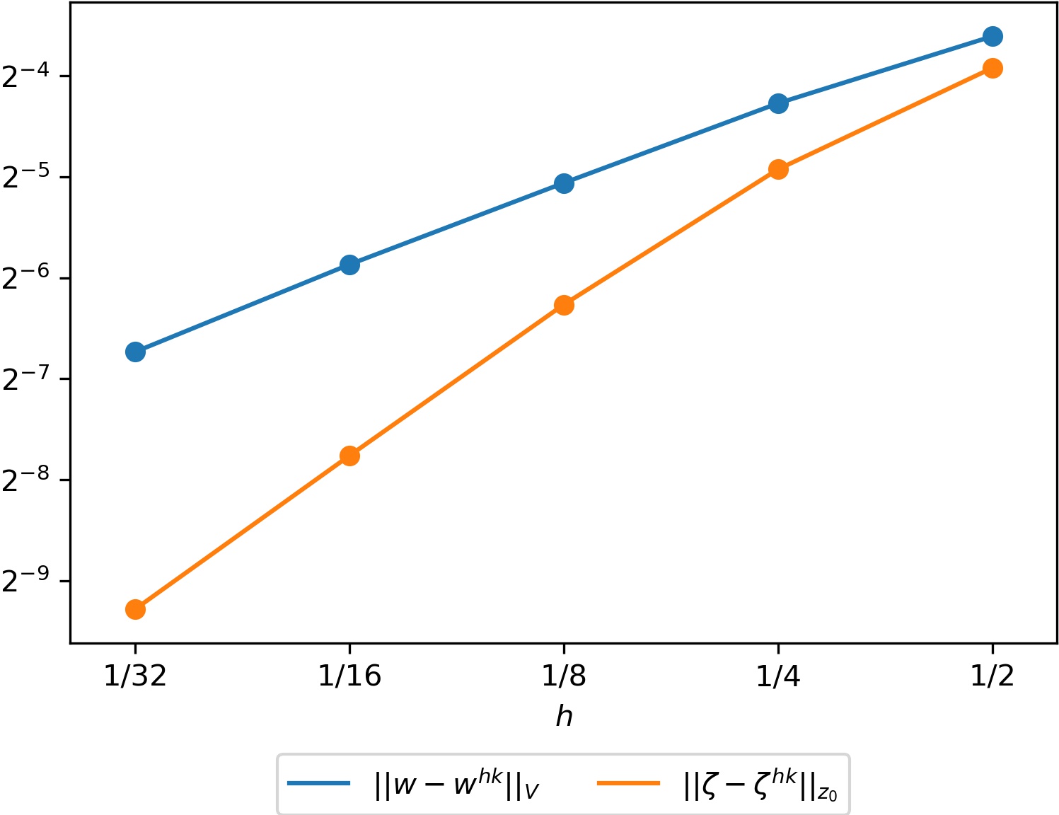
‖𝒘−𝒘h​k‖V/‖𝒘‖V\|\bm{w}-\bm{w}^{hk}\|_{V}/\|\bm{w}\|_{V} 3.4889​e−13.4889e-1 2.2027​e−12.2027e-1 1.2745​e−11.2745e-1 7.2811​e−27.2811e-2 3.9967​e−23.9967e-2
Convergence order 0.6635 0.7893 0.8077 0.8653
‖ζ−ζh​k‖V/‖ζ‖V\|\zeta-\zeta^{hk}\|_{V}/\|\zeta\|_{V} 8.7595​e−28.7595e-2 4.3672​e−24.3672e-2 1.7248​e−21.7248e-2 6.1124​e−36.1124e-3 2.1316​e−32.1316e-3
Convergence order 1.0041 1.3402 1.4966 1.5198
Table 1: Numerical errors vs. hh with fixed k=1/128k=1/128
kk 1/21/2 1/41/4 1/81/8 1/161/16 1/321/32
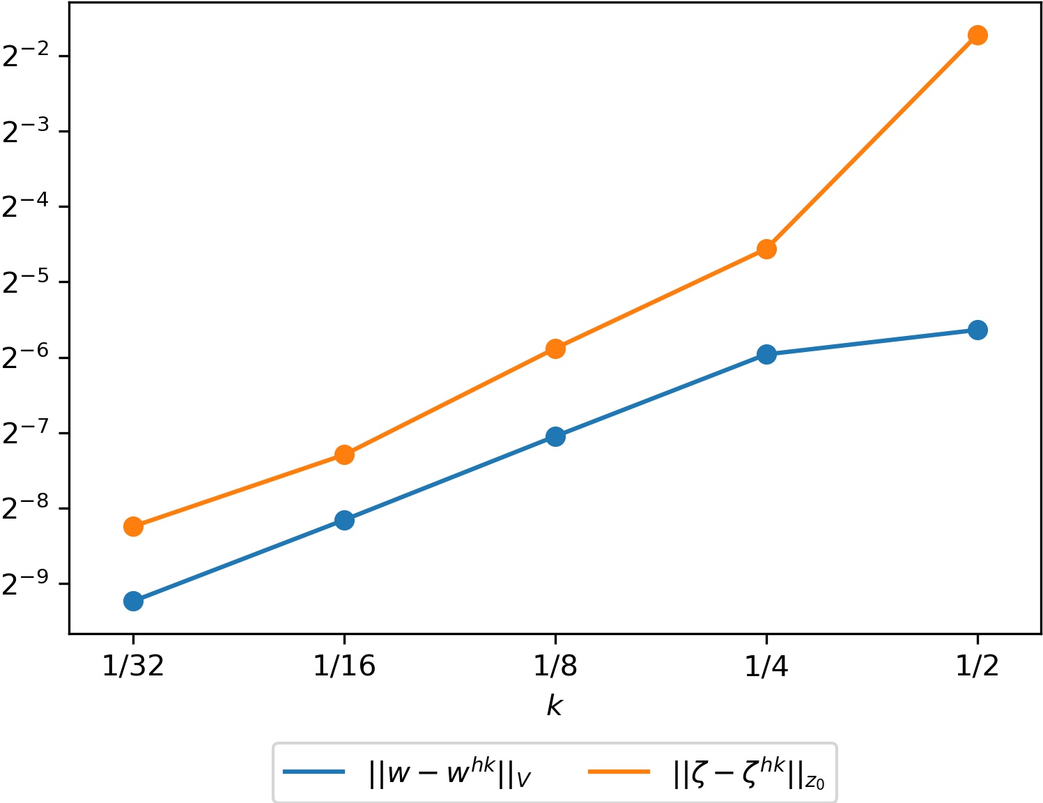
‖𝒘−𝒘h​k‖V/‖𝒘‖V\|\bm{w}-\bm{w}^{hk}\|_{V}/\|\bm{w}\|_{V} 8.5393​e−28.5393e-2 6.8195​e−26.8195e-2 3.2105​e−23.2105e-2 1.4883​e−21.4883e-2 7.0551​e−37.0551e-3
Convergence order 0.3244 1.0868 1.1091 1.0766
‖ζ−ζh​k‖V/‖ζ‖V\|\zeta-\zeta^{hk}\|_{V}/\|\zeta\|_{V} 4.0107​e−14.0107e-1 5.6124​e−25.6124e-2 2.2501​e−22.2501e-2 8.4583​e−38.4583e-3 4.3778​e−34.3778e-3
Convergence order 2.8372 1.3186 1.4115 0.9502
Table 2: Numerical errors vs. kk with fixed h=1/128h=1/128
Refer to caption
Figure 4: Errors vs. hh with fixed k=1/128k=1/128
Refer to caption
Figure 5: Errors vs. kk with fixed h=1/128h=1/128

We now turn to explore the convergence orders of the numerical solutions of a model problem. We take a square-shaped domain Ω=(0,1)×(0,1)\Omega=(0,1)\times(0,1), use the same data as in (4.1) and (4.2) and

Γ1={0}×[0,1],\displaystyle\Gamma_{1}=\{0\}\times[0,1],
OPENΓ2=([0,1]×{1})∪({1}×[0,1])),\displaystyle\Gamma_{2}=([0,1]\times\{1\})\cup(\{1\}\times[0,1])),
Γ3=[0,1]×{0},\displaystyle\Gamma_{3}=[0,1]\times\{0\},
𝒇0​(𝒙,t)=(0,0),𝒙∈Ω,t∈[0,T],\displaystyle\bm{f}_{0}(\bm{x},t)=(0,0),\quad\bm{x}\in\Omega,\ t\in[0,T],
𝒇2​(𝒙,t)=(−1.4,−0.2),𝒙∈Γ2,t∈[0,T].\displaystyle\bm{f}_{2}(\bm{x},t)=(-1.4,-0.2),\quad\bm{x}\in\Gamma_{2},\ t\in[0,T].

We use uniform triangulations of the spatial domain and uniform partitions of the time interval, and let hh and kk be the spatial mesh-size and time step-size as defined above. We present a comparison of numerical errors ‖𝒘−𝒘h​k‖V\|\bm{w}-\bm{w}^{hk}\|_{V} and ‖ζ−ζh​k‖Z0\|\zeta-\zeta^{hk}\|_{Z_{0}} computed for a sequence of numerical solutions. The numerical solution corresponding to h=1/128h=1/128 and k=1/128k=1/128 is taken as the “true” solution 𝒘\bm{w} and ζ\zeta in computing the numerical errors; ‖𝒘‖V≐0.23525\|\bm{w}\|_{V}\doteq 0.23525 and ‖ζ‖Z0≐0.75375\|\zeta\|_{Z_{0}}\doteq 0.75375.

First, we fix k=1/128k=1/128 and start with h=1/2h=1/2, which is successively halved. The results are presented in Table 1 and Figure 5, where the dependence of the relative error estimates ‖𝒘−𝒘h​k‖V\|\bm{w}-\bm{w}^{hk}\|_{V} and ‖ζ−ζh​k‖Z0\|\zeta-\zeta^{hk}\|_{Z_{0}} with respect to hh are plotted on a log-log scale. Asymptotic convergence orders close to one for the velocity variable and slightly higher for the damage variable can be observed for the numerical solutions.

Then, we fix h=1/128h=1/128 and start with k=1/2k=1/2, which is successively halved. The results are presented in Table 2 and Figure 5. Asymptotic convergence orders close to one for both unknowns can be observed.

Acknowledgments. The project has received funding from the European Union’s Horizon 2020 research and innovation programme under the Marie Skłodowska-Curie grant agreement No. 823731 CONMECH.

References

  • [1] K. Atkinson and W. Han, Theoretical Numerical Analysis: A Functional Analysis Framework, third edition, Springer, New York, 2009.
  • [2] M. Barboteu, K. Bartosz, W. Han, and T. Janiczko, Numerical analysis of a hyperbolic hemivariational inequality arising in dynamic contact, SIAM J. Numer. Anal. 53 (2015), 527–550.
  • [3] S. C. Brenner and L. R. Scott, The Mathematical Theory of Finite Element Methods, third edition, Springer-Verlag, New York, 2008.
  • [4] S. Carl, V. K. Le, and D. Motreanu, Nonsmooth Variational Problems and Their Inequalities: Comparison Principles and Applications, Springer, New York, 2007.
  • [5] P. G. Ciarlet, The Finite Element Method for Elliptic Problems, North Holland, Amsterdam, 1978.
  • [6] F. H. Clarke, Generalized gradients and applications, Trans. Amer. Math. Soc. 205 (1975), 247–262.
  • [7] F. H. Clarke, Optimization and Nonsmooth Analysis, Wiley, Interscience, New York, 1983.
  • [8] N. Cristescu and I. Suliciu, Viscoplasticity, Martinus Nijhoff Publishers, Editura Tehnica, Bucharest, 1982.
  • [9] M. Frémond, Non-Smooth Thermomechanics, Springer, Berlin, 2002.
  • [10] M. Frémond and B. Nedjar, Damage in concrete: the unilateral phenomenon, Nuclear Eng. Design 156 (1995), 323–335.
  • [11] M. Frémond and B. Nedjar, Damage, gradient of damage and principle of virtual work, Int. J. Solids Structures 33 (1996), 1083–1103.
  • [12] L. Gasiński, A. Ochal, and M. Shillor, Variational-hemivariational approach to a quasistatic viscoelastic problem with normal compliance, friction and material damage, Zeitschrift für Analysis und ihre Anwendungen 34 (2015), 251–275.
  • [13] W. Han, Numerical analysis of stationary variational-hemivariational inequalities with applications in contact mechanics, Mathematics and Mechanics of Solids 23 (2018), 279–293.
  • [14] W. Han, S. Migórski and M. Sofonea, A class of variational-hemivariational inequalities with applications to frictional contact problems, SIAM Journal of Mathematical Analysis 46 (2014), 3891–3912.
  • [15] W. Han, M. Shillor, and M. Sofonea, Variational and numerical analysis of a quasistatic viscoelastic problem with normal compliance, friction and damage, J. of Comp. and Applied Math. 137 (2001), 377–398.
  • [16] W. Han and M. Sofonea, Quasistatic Contact Problems in Viscoelasticity and Viscoplasticity, Studies in Advanced Mathematics, 30, American Mathematical Society, Providence, RI; International Press, Somerville, MA, 2002.
  • [17] W. Han and M. Sofonea, Numerical analysis of hemivariational inequalities in contact mechanics, Acta Numerica 28 (2019), 175–286.
  • [18] W. Han, M. Sofonea, and M. Barboteu, Numerical analysis of elliptic hemivariational inequalities, SIAM J. Numer. Anal. 55 (2017), 640–663.
  • [19] W. Han, M. Sofonea, and D. Danan, Numerical analysis of stationary variational-hemivariational inequalities, Numer. Math. 139 (2018), 563–592.
  • [20] J. Haslinger, M. Miettinen and P.D. Panagiotopoulos, Finite Element Method for Hemivariational Inequalities. Theory, Methods and Applications, Kluwer Academic Publishers, Boston, Dordrecht, London, 1999.
  • [21] I. Hlaváček, J. Haslinger, J. Nečas, and J. Lovíšek, Solution of Variational Inequalities in Mechanics, Springer-Verlag, New York, 1988.
  • [22] N. Kikuchi and J.T. Oden, Contact Problems in Elasticity: A Study of Variational Inequalities and Finite Element Methods, SIAM, Philadelphia, 1988.
  • [23] S. Migórski, A. Ochal, and M. Sofonea, Nonlinear Inclusions and Hemivariational Inequalities. Models and Analysis of Contact Problems, Advances in Mechanics and Mathematics 26, Springer, New York, 2013.
  • [24] Z. Naniewicz and P. D. Panagiotopoulos, Mathematical Theory of Hemivariational Inequalities and Applications, Dekker, New York, 1995.
  • [25] P. D. Panagiotopoulos, Nonconvex energy functions, hemivariational inequalities and substationary principles, Acta Mechanica 42 (1983), 160–183.
  • [26] P. D. Panagiotopoulos, Hemivariational Inequalities, Applications in Mechanics and Engineering, Springer–Verlag, Berlin, 1993.
  • [27] M. Sofonea, W. Han, and M. Shillor, Analysis and Approximation of Contact Problems with Adhesion or Damage, Chapman & Hall/CRC, New York, 2006.
  • [28] M. Sofonea and S. Migórski, Variational-Hemivariational Inequalities with Applications, Chapman & Hall/CRC Press, Boca Raton-London, 2018.