跳到论文正文
W Papers独立论文阅读器 arXiv:1912.07979 论文正文 计算阅读时间 · 0%
引用这篇论文根据当前论文元数据生成,正式投稿前建议核对。


License: CC BY 4.0
arXiv:1912.07979v2 [math.NT] 07 Aug 2023

Recursively divisible numbers

Thomas Fink Address: London Institute for Mathematical Sciences, Royal Institution, 21 Albemarle St, London W1S 4BS, UK
Date: August 11, 2026
Abstract.

We introduce and study the recursive divisor function, a recursive analog of the usual divisor function: κx(n)=nx+∑d⌊nκx(d)\kappa_{x}(n)=n^{x}+\sum_{d\lfloor n}\kappa_{x}(d), where the sum is over the proper divisors of nn. We give a geometrical interpretation of κx​(n)\kappa_{x}(n), which we use to derive a relation between κx​(n)\kappa_{x}(n) and κ0​(n)\kappa_{0}(n). For x≥2x\geq 2, we observe that κx​(n)/nx<1/(2−ζ⁡(x))\kappa_{x}(n)/n^{x}<1/(2-\zeta(x)). We show that, for n≥2n\geq 2, κ0​(n)\kappa_{0}(n) is twice the number of ordered factorizations, a problem much studied in its own right. By computing those numbers that are more recursively divisible than all of their predecessors, we recover many of the numbers prevalent in design and technology, and suggest new ones which have yet to be adopted.

1. Introduction

1.1. Recursive divisor function

In this paper we introduce and study the recursive divisor function:

Definition 1.
κx(n)=nx+∑d⌊nκ0(d),\kappa_{x}(n)=n^{x}+\sum_{d\lfloor n}\kappa_{0}(d),

where d⌊nd\lfloor n means d|nd|n and d<nd<n.

It can be thought of as the recursive analogue of the usual divisor function:

(1) σx​(n)=∑d|ndx.\sigma_{x}(n)=\sum_{d|n}d^{x}.

The recursive divisor function considers not only the divisors of nn, but also the divisors of the resultant quotients, and the divisors of those resultant quotients, and so on. For example, κ0​(10)=1+κ0​(1)+κ0​(2)+κ0​(5)=6\kappa_{0}(10)=1+\kappa_{0}(1)+\kappa_{0}(2)+\kappa_{0}(5)=6, and κ1​(10)=10+κ1​(1)+κ1​(2)+κ1​(5)=20\kappa_{1}(10)=10+\kappa_{1}(1)+\kappa_{1}(2)+\kappa_{1}(5)=20. Values of κ0,κ1\kappa_{0},\kappa_{1} and κ2\kappa_{2} are given in Table 1.

1.2. Example

Consider one of the earliest references to a number that can be divided into equal parts in many ways. Plato writes in his Laws that the ideal population of a city is 5040, since this number has more divisors than any number less than it. He observes that 5040 is divisible by 60 numbers, including one to 10. A highly divisible population is useful for dividing the city into equal-sized sectors for administrative, social and military purposes.
This conception of divisibility can be extended. Once the city is divided into equal parts, it is often necessary to divide a part into equal subparts. For example, if 5040 is divided into 15 parts of 336, each part can in turn be divided into subparts in 20 ways, since 336 has 20 divisors. But if 5040 is divided into 16 parts of 315, each part can be divided into subparts in only 12 ways, since 315 has 12 divisors. Thus the division of the whole into 15 parts offers more optionality for further subdivisions than the division into 16 parts. Similar reasoning can be applied to the division of the subparts into sub-subparts, and so on, in a recursive way.

nn κ0\kappa_{0} κ1\kappa_{1} κ2\kappa_{2}    nn κ0\kappa_{0} κ1\kappa_{1} κ2\kappa_{2}    nn κ0\kappa_{0} κ1\kappa_{1} κ2\kappa_{2}
1 1 1 1 21 6 34 502 41 2 42 1682
2 2 3 5 22 6 38 612 42 26 132 2636
3 2 4 10 23 2 24 530 43 2 44 1850
4 4 8 22 24 40 116 992 44 16 106 2698
5 2 6 26 25 4 32 652 45 16 96 2416
6 6 14 52 26 6 44 852 46 6 74 2652
7 2 8 50 27 8 46 832 47 2 48 2210
8 8 20 92 28 16 74 1114 48 96 304 4088
9 4 14 92 29 2 30 842 49 4 58 2452
10 6 20 132 30 26 104 1388 50 16 112 3316
11 2 12 122 31 2 32 962 51 6 74 2902
12 16 42 234 32 32 112 1520 52 16 122 3754
13 2 14 170 33 6 50 1222 53 2 54 2810
14 6 26 252 34 6 56 1452 54 40 190 4392
15 6 26 262 35 6 50 1302 55 6 74 3174
16 16 48 376 36 52 176 2196 56 40 196 4672
17 2 18 290 37 2 38 1370 57 6 82 3622
18 16 54 484 38 6 62 1812 58 6 92 4212
19 2 20 362 39 6 58 1702 59 2 60 3482
20 16 58 586 40 40 156 2464 60 88 346 6318
Table 1. Values of 𝜿𝟎,\kappa_{0}, 𝜿𝟏\kappa_{1} and 𝜿𝟐.\kappa_{2}. A Mathematica algorithm for 𝜿𝟎​(𝒏)\kappa_{0}(n) is: n = 1; 𝜿\kappa = {}; While[n <= 60, 𝜿\kappa = Append[𝜿\kappa, nˆ0 + Sum[𝜿\kappa[[m]], {m, Delete[Divisors[n], -1]}]]; n++]; 𝜿\kappa

1.3. Outline of paper

The goal of this paper is to quantify the notion of recursive divisibility and to understand the properties of numbers which possess it to a large degree. It is organized as follows.
In part 2, we introduce divisor trees (Figs. 1 and 2), which give a geometrical interpretation of κx​(n)\kappa_{x}(n). Using this, we find a relation between κx​(n)\kappa_{x}(n) and κ0​(n)\kappa_{0}(n).
In part 3, we show that for x≥2x\geq 2, κx​(n)<nx/(2−ζ⁡(x))\kappa_{x}(n)<n^{x}/(2-\zeta(x)). We plot κx​(n)\kappa_{x}(n) for x=1x=1 to x=6x=6, confirming our prediction.
In part 4, we investigate the number of recursive divisors κ0​(n)\kappa_{0}(n). We show that κ0​(n)\kappa_{0}(n) is twice the number of ordered factorizations for n≥2n\geq 2, a problem much studied in its own right [1, 2, 3, 4, 5, 6]. We give recursion relations for when nn is the product of distinct primes, and for when nn is the product of primes to a power. The latter can be solved for up to three primes.
In part 5, we investigate the sum of recursive divisors κ1​(n)\kappa_{1}(n). We give recursion relations for when nn is the product of primes to a power. These can be solved using the relation between κx​(n)\kappa_{x}(n) and κ0​(n)\kappa_{0}(n) from part 2.
In part 6, we study numbers which are recursively divisible to a high degree. We call numbers with a record number of recursive divisors recursively highly composite. These have been studied in the context of the number of ordered factorizations [6]. We call numbers with a record sum of recursive divisors, normalized by nn, recursively super-abundant. We list both kinds up to a million in Appendix A.
In part 7, we survey applications of highly recursive numbers in design and technology and display standards. We conclude with a list of open problems.

2. Divisor trees and the relation between κx\kappa_{x} and κ0\kappa_{0}

In this section, we prove the following relation between κx​(n)\kappa_{x}(n) and κ0​(n)\kappa_{0}(n):

Theorem 1.
κx​(n)nx=12+12​∑d|nκ0​(d)dx.\frac{\kappa_{x}(n)}{n^{x}}=\frac{1}{2}+\frac{1}{2}\sum_{d|n}\frac{\kappa_{0}(d)}{d^{x}}.

To do so, we introduce the concept of divisor trees. As well as motivating two lemmas necessary for our proof, divisor trees provide some intuition for how the recursive divisor function behaves.

Refer to caption
Figure 1. Divisor trees for 1 to 24. The number of recursive divisors κ0​(n)\kappa_{0}(n) counts the number of squares in each tree. The sum of recursive divisors κ1​(n)\kappa_{1}(n) adds up the side length of the squares in each tree. The sum of the square of recursive divisors κ2​(n)\kappa_{2}(n) adds up the area in each tree, and so on.

2.1. Divisor trees

A geometric interpretation of the recursive divisor function can be had by drawing the divisor tree for a given value of nn. Divisor trees for 1 to 24 are shown in Fig. 1. The number of recursive divisors κ0​(n)\kappa_{0}(n) counts the number of squares in each tree, whereas the number of divisors d≡σ0​(n)d\equiv\sigma_{0}(n) in (1) counts the number of squares in the main diagonal. The sum of recursive divisors κ1​(n)\kappa_{1}(n) adds up the side length of the squares in each tree, whereas the sum of divisors σ≡σ1​(n)\sigma\equiv\sigma_{1}(n) in (1) adds up the side length of the squares in the main diagonal. This can be extended to κ2​(n)\kappa_{2}(n), which adds up area, and so on.
A divisor tree is constructed as follows. First, draw a square of side length nn. Let d1,d2,…d_{1},d_{2},\ldots be the proper divisors of nn in descending order. Then draw squares of side length d1d_{1}, d2,…d_{2},\ldots with each consecutive square situated to the upper right of its predecessor, kitty-corner, as shown in Figs. 1 and 2. This forms the main arm of a divisor tree. Now, for each of the squares of side length d1,d2,…d_{1},d_{2},\ldots, repeat the process. Let e1,e2,…e_{1},e_{2},\ldots be the proper divisors of d1d_{1} in descending order. Then draw squares of side length e1e_{1}, e2,…e_{2},\ldots, but with the sub-arm rotated 90∘90^{\circ} counter-clockwise. Do the same for each of the remaining squares in the main arm. This forms the branches off of the main arm. Now, continue repeating this process, drawing arms off of arms off of arms, and so on, until the arms are single squares of size 1.
Note that, for large enough nn, a divisor tree can overlap itself. The precise conditions as to when is one of the open questions listed at the end.

2.2. Properties of divisor trees

In order to prove Theorem 1, let us consider a more fine-grained description of divisor trees, namely, one that counts the number of divisors of a given size.

Definition 2.

The number of recursive divisors of nn of size j<nj<n is

κ0​(n,j)={∑d⌊nκ0(d,j),j⌊n0,otherwise,\kappa_{0}(n,j)=\begin{cases}\displaystyle\sum_{d\lfloor n}\kappa_{0}(d,j),&j\lfloor n\\ 0,&{\rm otherwise},\end{cases}

where κ0​(n,n)=1\kappa_{0}(n,n)=1 and d⌊nd\lfloor n means d|nd|n and d<nd<n.

Lemma 1.

The number of recursive divisors of size jj satisifes κ0​(j​n,j)=κ0​(n,1)\kappa_{0}(j\,n,j)=\kappa_{0}(n,1).

Proof. By Definition 2, with j→1j\rightarrow 1,

(2) κ0(n,1)=∑d⌊nκ0(d,1).\kappa_{0}(n,1)=\sum_{d\lfloor n}\kappa_{0}(d,1).

Similarly, with n→j​nn\rightarrow j\,n,

κ0(jn,j)=∑d⌊jnκ0(d,j).\kappa_{0}(j\,n,j)=\sum_{d\lfloor j\,n}\kappa_{0}(d,j).

Since κ0​(d,j)=0\kappa_{0}(d,j)=0 if jj does not divide dd, this can be rewritten as

(3) κ0(jn,j)=∑d⌊nκ0(jd,j).\kappa_{0}(j\,n,j)=\sum_{d\lfloor n}\kappa_{0}(j\,d,j).

We will use this result in a moment.
Let n=p1α1​p2α2​…​pωαjn=p_{1}^{\alpha_{1}}\,p_{2}^{\alpha_{2}}\ldots p_{\omega}^{\alpha_{j}} and Ω⁡(n)=α1+α2+…+αω\Omega(n)=\alpha_{1}+\alpha_{2}+\ldots+\alpha_{\omega}. We prove the lemma by induction on Ω⁡(n)\Omega(n). The base case Ω⁡(n)=0\Omega(n)=0, or n=1n=1, holds by Definition 2: κ0​(j​ 1,j)=κ0​(1,1)\kappa_{0}(j\,1,j)=\kappa_{0}(1,1). We now show that if κ0​(j​n,j)=κ0​(n,1)\kappa_{0}(j\,n,j)=\kappa_{0}(n,1) for all nn such that Ω⁡(n)<i\Omega(n)<i, then κ0​(j​n,j)=κ0​(n,1)\kappa_{0}(j\,n,j)=\kappa_{0}(n,1) for all nn such that Ω⁡(n)<i+1\Omega(n)<i+1. To see why, observe that in (3) all of the proper divisors dd of nn must have Ω⁡(d)\Omega(d) at most Ω⁡(n)−1\Omega(n)-1. So by assumption all of the κ0​(j​d,j)\kappa_{0}(j\,d,j) in (3) reduce to κ0​(d,1)\kappa_{0}(d,1), and the right side of (3) takes the form of the right side of (2) and thus equals κ0​(n,1)\kappa_{0}(n,1). ∎

Refer to caption
Figure 2. Divisor trees for 96 and 100. There are κ0​(96)=224\kappa_{0}(96)=224 squares in the left tree and κ0​(100)=52\kappa_{0}(100)=52 squares in the right tree. The sum of the side length of the squares, or one-fourth of the tree perimeter, is κ1​(96)=768\kappa_{1}(96)=768 and κ1​(100)=340\kappa_{1}(100)=340. The sum of the area of the squares is κ2​(96)=\kappa_{2}(96)= 16,608 and κ2​(100)=\kappa_{2}(100)= 14,740.
Lemma 2.

For n≥2n\geq 2, the number of recursive divisors of size 1 is equal to half the total number of recursive divisors, that is, κ0​(n,1)=κ0​(n)/2\kappa_{0}(n,1)=\kappa_{0}(n)/2.

Proof. Clearly

κ0​(n)=∑d|nκ0​(n,d).\kappa_{0}(n)=\sum_{d|n}\kappa_{0}(n,d).

By Lemma 1, κ0​(n,k)=κ0​(n/k,1)\kappa_{0}(n,k)=\kappa_{0}(n/k,1) for k|nk|n, so the above becomes

κ0​(n)\displaystyle\kappa_{0}(n) =∑d|nκ0​(n/d,1)\displaystyle=\sum_{d|n}\kappa_{0}(n/d,1)
=∑d|nκ0​(d,1)\displaystyle=\sum_{d|n}\kappa_{0}(d,1)
=κ0(n,1)+∑d⌊nκ0(d,1).\displaystyle=\kappa_{0}(n,1)+\sum_{d\lfloor n}\kappa_{0}(d,1).

Inserting Definition 2 with j=1j=1 into the above gives the desired result. ∎

2.3. Relation between 𝜿𝒙\kappa_{x} and 𝜿𝟎\kappa_{0}.

Proof of Theorem 1. We can write κx​(n)\kappa_{x}(n) as

κx​(n)=∑d|ndx​κ0​(n,d).\kappa_{x}(n)=\sum_{d|n}d^{x}\,\kappa_{0}(n,d).

By Lemma 1,

κx​(n)=∑d|ndx​κ0​(n/d,1).\kappa_{x}(n)=\sum_{d|n}d^{x}\,\kappa_{0}(n/d,1).

Recall that Lemma 2 only applies for n≥2n\geq 2, so we pull out the d=nd=n term:

κx(n)=nx+∑d⌊ndxκ0(n/d,1).\kappa_{x}(n)=n^{x}+\sum_{d\lfloor n}d^{x}\,\kappa_{0}(n/d,1).

By Lemma 2,

κx​(n)\displaystyle\kappa_{x}(n) =nx+12∑d⌊ndxκ0(n/d)\displaystyle=n^{x}+\frac{1}{2}\sum_{d\lfloor n}d^{x}\,\kappa_{0}(n/d)
=nx2+12​∑d|ndx​κ0​(n/d)\displaystyle=\frac{n^{x}}{2}+\frac{1}{2}\sum_{d|n}d^{x}\kappa_{0}(n/d)
=nx2+12​∑d|n(nd)x​κ0​(d).\displaystyle=\frac{n^{x}}{2}+\frac{1}{2}\sum_{d|n}\left(\frac{n}{d}\right)^{x}\kappa_{0}(d).

Dividing by nxn^{x}, the theorem follows. ∎

Refer to caption
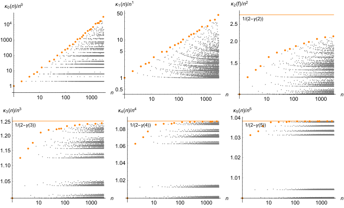
Figure 3. Plots of 𝜿𝒙​(𝒏)/𝒏𝒙.\kappa_{x}(n)/n^{x}. We plot 𝜿𝒙​(𝒏)/𝒏𝒙\kappa_{x}(n)/n^{x} up to 𝒏=n= 3,000, for 𝒙=𝟎x=0 to 𝒙=𝟓x=5. The large orange points are the sequence records, which satisfy 𝜿𝒙​(𝒏)/𝒏𝒙>𝜿𝒙​(𝒎)/𝒎𝒙\kappa_{x}(n)/n^{x}>\kappa_{x}(m)/m^{x} for all 𝒎<𝒏m<n. For 𝒙=𝟎x=0 and 𝒙=𝟏x=1, the upper bound for the sequence diverges. But for 𝒙=𝟐x=2 and above, it converges to 𝟏/(𝟐−𝜸⁡(𝒙))1/(2-\gamma(x)), where 𝜸\gamma is the Riemann zeta function. For 𝒙=𝟎x=0, the orange points are the recursively highly composite numbers. For 𝒙=𝟏x=1, they are the recursively super-abundnant numbers (see Appendix A).

3. Properties of κ2\kappa_{2}, κ3\kappa_{3}, and so on.

Theorem 2.

For x>1x>1,

κx​(n)nx<12−ζ⁡(x).\frac{\kappa_{x}(n)}{n^{x}}<\frac{1}{2-\zeta(x)}.

This theorem was inspired by an anonymous referee from a previous version of this paper. The referee answered one of our then open questions at the end of our paper. We generalized the answer, which led to this theorem. We confirm it in Fig. 3, in which we plot κx​(n)/nx\kappa_{x}(n)/n^{x} for x=1x=1 to x=6x=6.
Proof. We prove the theorem by induction. We know that it is true for n=1n=1. Assume it is true for all numbers less than nn. We show it is then true for nn. By Definition 1,

κx​(n)nx\displaystyle\frac{\kappa_{x}(n)}{n^{x}} =\displaystyle= 1+1nx∑d⌊nκx(d)\displaystyle 1+\frac{1}{n^{x}}\sum_{d\lfloor n}\kappa_{x}(d)
=\displaystyle= 1+∑d⌊nκx​(d)dxdxnx\displaystyle 1+\sum_{d\lfloor n}\frac{\kappa_{x}(d)}{d^{x}}\frac{d^{x}}{n^{x}}
<\displaystyle< 1+12−ζ⁡(x)∑d⌊ndxnx\displaystyle 1+\frac{1}{2-\zeta(x)}\sum_{d\lfloor n}\frac{d^{x}}{n^{x}}
<\displaystyle< 1+12−ζ⁡(x)​(−1+∑d|ndxnx),\displaystyle 1+\frac{1}{2-\zeta(x)}\Bigg(-1+\sum_{d|n}\frac{d^{x}}{n^{x}}\Bigg),

where γ⁡(x)\gamma(x) is the Riemann zeta function. Since, for x>1x>1,

(4) ∑d|ndxnx=∑d|n1dx<ζ⁡(x),\sum_{d|n}\frac{d^{x}}{n^{x}}=\sum_{d|n}\frac{1}{d^{x}}<\zeta(x),

we have

κx​(n)nx\displaystyle\frac{\kappa_{x}(n)}{n^{x}} <\displaystyle< 1+12−ζ⁡(x)​(ζ​(x)−1)\displaystyle 1+\frac{1}{2-\zeta(x)}\left(\zeta(x)-1\right)
<\displaystyle< 12−ζ⁡(x).∎\displaystyle\frac{1}{2-\zeta(x)}.\quad\qed

4. Number of recursive divisors

4.1. Relation to ordered factorizations

Some of the properties of κ0​(n)\kappa_{0}(n) can be deduced from properties of a related function, the number K⁡(n)K(n) of ordered factorizations into integers greater than one. It satisfies K⁡(1)=1K(1)=1 and

K(n)=∑d⌊nK(d).K(n)=\sum_{d\lfloor n}K(d).

For example, 12 is the product of integers greater than one in eight ways: 12=6⋅2=2⋅6=4⋅3=3⋅4=3⋅2⋅2=2⋅3⋅2=2⋅2⋅312=6\cdot 2=2\cdot 6=4\cdot 3=3\cdot 4=3\cdot 2\cdot 2=2\cdot 3\cdot 2=2\cdot 2\cdot 3. So K⁡(12)=8K(12)=8. Kalmar [1] was the first to consider K⁡(n)K(n)—hence the name KK—and it was later studied more systematically by Hille [2]. Over the last 20 years several authors have extended Hille’s results [4, 5, 6], some of which we will mention later.
Notice that the definition of K⁡(n)K(n) is identical to Definition 2 for j=1j=1, that is, to κ0​(n,1)\kappa_{0}(n,1). Since K⁡(1)=κ0​(1,1)=1K(1)=\kappa_{0}(1,1)=1, then by Lemma 2 we arrive at

Proposition 1.

For n≥2n\geq 2, κ0​(n)=2​K​(n)\kappa_{0}(n)=2K(n), where K⁡(n)K(n) is the number of ordered factorizations into integers greater than one.

4.2. Distinct primes

Let n=p1​p2​…​pωn=p_{1}p_{2}\ldots p_{\omega} be the product of ω\omega distinct primes.

Proposition 2.

The exponential generating function of κ0​(p1​…​pω)\kappa_{0}(p_{1}\ldots p_{\omega}) is

EG⁡(κ0​(p1​…​pω),x)=ex2−ex.{\rm EG}(\kappa_{0}(p_{1}\ldots p_{\omega}),x)=\frac{e^{x}}{2-e^{x}}.

Proof. Since κ0\kappa_{0} depends only on the prime signature of nn, which in this case is all 1s, we can immediately write down

2​κ0​(p1​…​pω)=1+∑i=0ω(ωi)​κ0​(p1​…​pi).2\kappa_{0}(p_{1}\ldots p_{\omega})=1+\sum_{i=0}^{\omega}\binom{\omega}{i}\kappa_{0}(p_{1}\ldots p_{i}).

Then

2​∑ω=0∞xww!​κ0​(p1,…,pω)\displaystyle 2\sum_{\omega=0}^{\infty}\frac{x^{w}}{w!}\kappa_{0}(p_{1},\ldots,p_{\omega}) =∑ω=0∞xωω!​(1+∑i=0ω(ωi)​κ0​(p1​…​pi))\displaystyle=\sum_{\omega=0}^{\infty}\frac{x^{\omega}}{\omega!}\left(1+\sum_{i=0}^{\omega}\binom{\omega}{i}\kappa_{0}(p_{1}\ldots p_{i})\right)
=ex+∑ω=0∞∑i=0ωxii!​xω−i(ω−i)!​κ0​(p1​…​pi).\displaystyle=e^{x}+\sum_{\omega=0}^{\infty}\sum_{i=0}^{\omega}\frac{x^{i}}{i!}\frac{x^{\omega-i}}{(\omega-i)!}\kappa_{0}(p_{1}\ldots p_{i}).

Summing this along the diagonals ω=i\omega=i, ω=i+1\omega=i+1, and so on,

2​∑ω=0∞xww!​κ0​(p1,…,pω)\displaystyle 2\sum_{\omega=0}^{\infty}\frac{x^{w}}{w!}\kappa_{0}(p_{1},\ldots,p_{\omega}) =ex+x00!​∑ω=0∞xww!​κ0​(p1,…,pω)+x11!​∑ω=0∞xww!​κ0​(p1,…,pω)+…\displaystyle\!=\!e^{x}\!+\!\frac{x^{0}}{0!}\sum_{\omega=0}^{\infty}\frac{x^{w}}{w!}\kappa_{0}(p_{1},\ldots,p_{\omega})\!+\!\frac{x^{1}}{1!}\sum_{\omega=0}^{\infty}\frac{x^{w}}{w!}\kappa_{0}(p_{1},\ldots,p_{\omega})\!+\!\ldots
=ex+ex​∑ω=0∞xww!​κ0​(p1,…,pω).\displaystyle=e^{x}+e^{x}\sum_{\omega=0}^{\infty}\frac{x^{w}}{w!}\kappa_{0}(p_{1},\ldots,p_{\omega}).

From this it follows that

EG⁡(κ0​(p1​…​pω),x)=ex2−ex.∎{\rm EG}(\kappa_{0}(p_{1}\ldots p_{\omega}),x)=\frac{e^{x}}{2-e^{x}}.\qed

4.3. Primes to a power

When nn is the product of primes to powers, κ0​(n)\kappa_{0}(n) satisfies recursion relations relating it to values of κ0​(n)\kappa_{0}(n) for primes to lower powers. The first few of these can be solved explicitly.

Theorem 3.

Let p,qp,q and rr be prime. Then

κ0​(pc)\displaystyle\kappa_{0}(p^{c}) =2​κ0​(pcp)\displaystyle=\textstyle 2\kappa_{0}\big(\frac{p^{c}}{p}\big)
=2c\displaystyle=2^{c}
κ0​(pc​qd)\displaystyle\kappa_{0}(p^{c}q^{d}) =2​(κ0​(pc​qdp)+κ0​(pc​qdq)−κ0​(pc​qdp​q))\displaystyle=2\left(\textstyle\kappa_{0}\big(\frac{p^{c}q^{d}}{p}\big)+\kappa_{0}\big(\frac{p^{c}q^{d}}{q}\big)-\kappa_{0}\big(\frac{p^{c}q^{d}}{pq}\big)\right)
=2c​∑i=0d(di)​(c+ii),\displaystyle=2^{c}\sum_{i=0}^{d}\textstyle\binom{d}{i}\binom{c+i}{i},
κ0​(pc​qd​re)\displaystyle\kappa_{0}(p^{c}q^{d}r^{e}) =2​(κ0​(pc​qd​rep)+κ0​(pc​qd​req)+κ0​(pc​qd​rer)CLOSE\displaystyle=2\Big(\textstyle\kappa_{0}\big(\frac{p^{c}q^{d}r^{e}}{p}\big)+\kappa_{0}\big(\frac{p^{c}q^{d}r^{e}}{q}\big)+\kappa_{0}\big(\frac{p^{c}q^{d}r^{e}}{r}\big)
OPEN−κ0​(pc​qd​rep​q)−κ0​(pc​qd​rep​r)−κ0​(pc​qd​req​r)+κ0​(pc​qd​rep​q​r))\displaystyle\textstyle-\kappa_{0}\big(\frac{p^{c}q^{d}r^{e}}{pq}\big)-\kappa_{0}\big(\frac{p^{c}q^{d}r^{e}}{pr}\big)-\kappa_{0}\big(\frac{p^{c}q^{d}r^{e}}{qr}\big)+\kappa_{0}\big(\frac{p^{c}q^{d}r^{e}}{pqr}\big)\Big)
=∑j=0d(−1)j​(dj)​(c+d−jd)​κ0​(pc+d−j​re).\displaystyle=\sum_{j=0}^{d}(-1)^{j}\textstyle\binom{d}{j}\binom{c+d-j}{d}\kappa_{0}(p^{c+d-j}r^{e}).

Analogous recursion relations apply for the product of more primes to powers.

Proof. For the recursion relations, the approach is similar to, but somewhat simpler than, that used to prove the recursion relations in Theorem 4. But we can deduce these relations from previous work using Proposition 1. Hille [2] and Chor et al. [4] proved that identical recursion relations govern K⁡(n)K(n), the number of ordered factorizations. Since κ0​(n)=2​K​(n)\kappa_{0}(n)=2K(n) for n≥2n\geq 2, the same recursion relations apply to κ0​(n)\kappa_{0}(n). For the explicit forms of κ0\kappa_{0}, Chor et al. [4] give analogous results for K⁡(n)K(n), which when multiplied by 2 apply to κ0​(n)\kappa_{0}(n). ∎

Corollary 1.

Let α∗\alpha^{*} be the maximum exponent in the prime factorization of nn. Then 2α∗2^{\alpha^{*}} divides κ0​(n)\kappa_{0}(n).

Proof. All of the recursion relations in Theorem 3 have a factor of 2 on the right side. The corollary is implied by iterating the recursion relation α∗\alpha^{*} times. Each time, the exponents on the right are reduced by at most 1. Iterating until the smallest exponent is reduced to 0, the exponent disappears since, for example, κ0​(pc​q0)=κ0​(pc)\kappa_{0}(p^{c}q^{0})=\kappa_{0}(p^{c}). Continuing this process ultimately gives a total of α∗\alpha^{*} factors of 2. The κ0​(n)\kappa_{0}(n) are expressed as a product of an integer and 2α∗2^{\alpha^{*}} in Appendix A. ∎

5. Sum of recursive divisors

We now turn to the sum of recursive divisors κ1​(n)\kappa_{1}(n). This quantity is more intricate than κ0​(n)\kappa_{0}(n), because it depends on the primes as well as their exponents in the prime factorization of nn.

5.1. Primes to a power

When nn is equal to the product of primes to powers, κ1​(n)\kappa_{1}(n) satisfies recursion relations similar to those for κ0​(n)\kappa_{0}(n), but more complex.

Theorem 4.

Let p,qp,q and rr be prime. Then

κ1​(pc)\displaystyle\kappa_{1}(p^{c}) =2​κ1​(pcp)+p−1p​pc\displaystyle=\textstyle 2\kappa_{1}\big(\frac{p^{c}}{p}\big)+\frac{p-1}{p}p^{c}
={2c​c+22p=2pc​p−1−(2/p)cp−2p​odd\displaystyle=\begin{cases}2^{c}\,\frac{c+2}{2}&p=2\\ p^{c}\,\frac{p-1-(2/p)^{c}}{p-2}&p\;{\rm odd}\end{cases}
κ1​(pc​qd)\displaystyle\kappa_{1}(p^{c}q^{d}) =2​(κ1​(pc​qdp)+κ1​(pc​qdq)−κ1​(pc​qdp​q))+p−1p​q−1q​pc​qd\displaystyle=\textstyle 2\left(\kappa_{1}\big(\frac{p^{c}q^{d}}{p}\big)+\kappa_{1}\big(\frac{p^{c}q^{d}}{q}\big)-\kappa_{1}\big(\frac{p^{c}q^{d}}{pq}\big)\right)+\frac{p-1}{p}\frac{q-1}{q}p^{c}q^{d}
=pc​qd​(12+12​∑i=0c2ipi​∑j=0d1qj​∑k=0j(i+kk)​(jk))\displaystyle=p^{c}q^{d}\bigg(\frac{1}{2}+\frac{1}{2}\sum_{i=0}^{c}\frac{2^{i}}{p^{i}}\sum_{j=0}^{d}\frac{1}{q^{j}}\sum_{k=0}^{j}\textstyle\binom{i+k}{k}\binom{j}{k}\bigg)
κ1​(pc​qd​re)\displaystyle\kappa_{1}(p^{c}q^{d}r^{e}) =2​(κ1​(pc​qd​rep)+κ1​(pc​qd​req)+κ1​(pc​qd​rer)CLOSE\displaystyle=2\Big(\textstyle\kappa_{1}\big(\frac{p^{c}q^{d}r^{e}}{p}\big)+\kappa_{1}\big(\frac{p^{c}q^{d}r^{e}}{q}\big)+\kappa_{1}\big(\frac{p^{c}q^{d}r^{e}}{r}\big)
OPEN−κ1​(pc​qd​rep​q)−κ1​(pc​qd​rep​r)−κ1​(pc​qd​req​r)+κ1​(pc​qd​rep​q​r))\displaystyle\textstyle-\kappa_{1}\big(\frac{p^{c}q^{d}r^{e}}{pq}\big)-\kappa_{1}\big(\frac{p^{c}q^{d}r^{e}}{pr}\big)-\kappa_{1}\big(\frac{p^{c}q^{d}r^{e}}{qr}\big)+\kappa_{1}\big(\frac{p^{c}q^{d}r^{e}}{pqr}\big)\Big)
+p−1p​q−1q​r−1r​pc​qd​re.\displaystyle\textstyle+\frac{p-1}{p}\frac{q-1}{q}\frac{r-1}{r}p^{c}q^{d}r^{e}.

Proof. We start with the recursion relations. For n=pcn=p^{c}, from Definition 1,

(5) κ1​(pc)=pc+∑i=0c−1κ1​(pi).\kappa_{1}(p^{c})=p^{c}+\sum_{i=0}^{c-1}\kappa_{1}(p^{i}).

Adding κ1​(pc)\kappa_{1}(p^{c}) to both sides and with c→c−1c\rightarrow c-1,

∑i=0c−1κ1​(pi)=2​κ1​(pc−1)−pc−1,\sum_{i=0}^{c-1}\kappa_{1}(p^{i})=2\kappa_{1}(p^{c-1})-p^{c-1},

which, when inserted into (5), gives the desired recurrence relation.
For n=pc​qdn=p^{c}q^{d}, from Definition 1,

(6) κ1​(pc​qd)=pc​qd+∑i=0c−1∑j=0dκ1​(pi​qj)+∑j=0d−1κ1​(pc​qj).\kappa_{1}(p^{c}q^{d})=p^{c}q^{d}+\sum_{i=0}^{c-1}\sum_{j=0}^{d}\kappa_{1}(p^{i}q^{j})+\sum_{j=0}^{d-1}\kappa_{1}(p^{c}q^{j}).

Adding κ1​(pc​qd)\kappa_{1}(p^{c}q^{d}) to both sides,

(7) 2​κ1​(pc​qd)=pc​qd+∑i=0c−1∑j=0dκ1​(pi​qj)+∑j=0dκ1​(pc​qj),2\kappa_{1}(p^{c}q^{d})=p^{c}q^{d}+\sum_{i=0}^{c-1}\sum_{j=0}^{d}\kappa_{1}(p^{i}q^{j})+\sum_{j=0}^{d}\kappa_{1}(p^{c}q^{j}),

which we can equally write

(8) 2​κ1​(pc​qd)=pc​qd+∑i=0c∑j=0dκ1​(pi​qj).2\kappa_{1}(p^{c}q^{d})=p^{c}q^{d}+\sum_{i=0}^{c}\sum_{j=0}^{d}\kappa_{1}(p^{i}q^{j}).

With d→d−1d\rightarrow d-1 in (7), we find

(9) ∑j=0d−1κ1​(pc​qj)=2​κ1​(pc​qd−1)−pc​qd−1−∑j=0c−1∑i=0d−1κ1​(pi​qj).\sum_{j=0}^{d-1}\kappa_{1}(p^{c}q^{j})=2\kappa_{1}(p^{c}q^{d-1})-p^{c}q^{d-1}-\sum_{j=0}^{c-1}\sum_{i=0}^{d-1}\kappa_{1}(p^{i}q^{j}).

With c→c−1c\rightarrow c-1 and d→d−1d\rightarrow d-1 in (8), and inserting the result into (9), yields

(10) ∑j=0d−1κ1​(pc​qj)=2​κ1​(pc​qd−1)−2​κ1​(pc−1​qd−1)+(1−p)​pc−1​qd−1.\sum_{j=0}^{d-1}\kappa_{1}(p^{c}q^{j})=2\kappa_{1}(p^{c}q^{d-1})-2\kappa_{1}(p^{c-1}q^{d-1})+(1-p)p^{c-1}q^{d-1}.

With c→c−1c\rightarrow c-1 in (8), we find

(11) ∑i=0c−1∑j=0dκ1​(pi​qj)=2​κ1​(pc−1​qd)−pc−1​qd.\sum_{i=0}^{c-1}\sum_{j=0}^{d}\kappa_{1}(p^{i}q^{j})=2\kappa_{1}(p^{c-1}q^{d})-p^{c-1}q^{d}.

Inserting (10) and (11) into (6) gives the desired recursion relation.
For n=pc​qd​ren=p^{c}q^{d}r^{e}, the proof is similar to the one above and is omitted here.
For the explicit forms of κ1​(n)\kappa_{1}(n), we appeal to Theorem 1, which tells us

(12) 2​κ1​(n)n=1+∑d|nκ0​(d)d.\frac{2\kappa_{1}(n)}{n}=1+\sum_{d|n}\frac{\kappa_{0}(d)}{d}.

For n=pcn=p^{c}, from (12) we have

2​κ1​(pc)pc=1+∑i=0cκ0​(pi)pi.\frac{2\kappa_{1}(p^{c})}{p^{c}}=1+\sum_{i=0}^{c}\frac{\kappa_{0}(p^{i})}{p^{i}}.

Inserting Theorem 3 into the above gives the desired result. For n=pc​qdn=p^{c}q^{d}, from (12) we have

2​κ1​(pc​qd)pc​qd=1+∑i=0c∑j=0dκ0​(pi​qj)pi​qj.\frac{2\kappa_{1}(p^{c}q^{d})}{p^{c}q^{d}}=1+\sum_{i=0}^{c}\sum_{j=0}^{d}\frac{\kappa_{0}(p^{i}q^{j})}{p^{i}q^{j}}.

Inserting Theorem 3 into the above gives the desired result. For p=2p=2, the result simplifies to contain just two sums. ∎

6. Numbers that are recursively divisible to a high degree

6.1. Recursively highly composite numbers

A number nn is highly composite [7] if it has more divisors than any of its predecessors, that is, σ0​(n)>σ0​(m)\sigma_{0}(n)>\sigma_{0}(m) for all m<nm<n. These are shown in the right side of Table 2 in Appendix A.
By analogy with highly composite numbers, a number nn is recursively highly composite if it has more recursive divisors than any of its predecessors.

Definition 3.

nn is recursively highly composite if κ0​(n)>κ0​(m)\kappa_{0}(n)>\kappa_{0}(m) for all m<nm<n.

These numbers are shown in the left side of Table 2 in Appendix A. From the third term, they correspond to the indices of sequence records of K⁡(n)K(n), the K-champion numbers [6]. Because κ0​(n)\kappa_{0}(n) depends only on the exponents in the prime factorization of nn, the exponents in recursively highly composite numbers must be non-increasing.

6.2. Recursively super-abundant numbers

A number nn is super-abundant [8] if the sum of its divisors, normalized by nn, is greater than that of any of its predecessors, that is, σ⁡(n)/n>σ⁡(m)/m\sigma(n)/n>\sigma(m)/m for all m<nm<n. These are the starred numbers in the right side of Table 2 in Appendix A. For small nn, super-abundant numbers are also highly composite, but later this ceases to be the case. The first super-abundant number that is not highly composite is 1,163,962,800 (A166735 [9]), and in fact only 449 numbers have both properties (A166981 [9]).
By analogy with super-abundant numbers, a number nn is recursively super-abundant if the sum of its recursive divisors, normalized by nn, is greater than that of any of its predecessors.

Definition 4.

nn is recursively super-abundant if κ1​(n)/n>κ1​(m)/m\kappa_{1}(n)/n>\kappa_{1}(m)/m for all m<nm<n.

These numbers are starred in the left side of Table 2 in Appendix A. Early on, recursively super-abundant numbers are recursively highly composite. The first exception is 181,440.

nn Design and technology Display standards
24 24×1624\times 16 Biotech 384-well assay
48 128×48128\times 48 TRS 80
72 72 points/in Adobe typography point
96 96×6596\times 65 Nokia 1100 phone
120 120×160120\times 160 Nokia 100 phone 160×120160\times 120 QQVGA
144 144×168144\times 168 Pebble Time watch
240 240×64240\times 64 Atari Portfolio 320×240320\times 240 Quarter VGA
288 352×288352\times 288 Video CD 352×288352\times 288 CIF
360 360×360360\times 360 LG Watch Style 640×360640\times 360 nHD
480 320×480320\times 480 iPhone 1–3 640×480640\times 480 VGA
576 576 lines PAL analog television 1024×5761024\times 576 WSVGA
720 720×364720\times 364 Macintosh XL, Hercules 1280×7201280\times 720 HD
864 1152×8641152\times 864 XGA+
960 Facebook website
1152 1152×20481152\times 2048 QWXGA
1440 3.5” disk block size 2560×14402560\times 1440 Quad HD
1920 1920×10801920\times 1080 Full HD
2160 2160×14402160\times 1440 Microsoft Surface Pro 3 4096×21604096\times 2160 4K Ultra HD
2304 2304×14402304\times 1440 MacBook Retina
2880 2880×1800\hskip 9.24994pt2880\times 1800 15” MacBook Pro Retina     5120×28805120\times 2880 5K
3456 Canon EOS 1100D
4320 7680×43207680\times 4320 8K Ultra HD
8640 15360×864015360\times 8640 16K Ultra HD
Table 3. Applications. Numbers that are recursively divisible to a large degree predict the numbers that frequently show up in design and technology and display standards. All of the numbers nn are recursively highly composite; those that are starred are also recursively super-abundant.

6.3. Applications.

In graphic and digital design, the layout of graphics and text is often constrained to lie on an underlying rectangular grid [10]. The grid elements are the primitive building blocks from which bigger columns or rows can be formed. For example, grids of 24 and 96 columns are often used for books and websites, respectively [10]. Using a grid reduces the space of possible designs, making it easier to navigate. And the design elements become more interoperable, like how Lego bricks snap into place with one another, making it faster to build new designs.
What are the best grid sizes? The challenge is committing to a grid size now that provides the greatest optionality for an unknown future. Imagine, for example, that we have to cut a pie into slices, to be divided up later for an unknown number of colleagues. How many slices should we choose? The answer in this case is straightforward: the best grids are the ones with the most divisors, such as the highly composite or super-abundant numbers [7, 8].
But the story gets more complicated when we need to consider steps into the future. For instance, imagine now that each colleague takes his share of pie home to further divide it amongst his family—but they cannot make any additional cuts. In this case, not only does the whole need to be highly divisible, but the parts need to be highly divisible, too. This process can be extended in a recursive way.
Recursive modularity, in which there are multiple levels of organization, has long been a feature of graphic and digital design. For example, newspapers are divided into columns for different stories, and columns into sub-columns of text. But with the rise of digital technologies, recursive modularity is becoming the rule. Different pages of a website are divided into different numbers of columns, each of which can be broken down into smaller design elements. Often one column from the website fills the full screen of a phone.
Specific applications of recursively highly composite numbers are shown in Table 3. In design and technology, these numbers are used for the screen resolutions of watches, phones, cameras and computers. They appear in typesetting, websites, and experimental equipment, such as test tube microplates. In display standards, many resolutions use these numbers in the height or width, measured in pixels. Because these standards tend to preserve certain aspect ratios, such as 16:9, usually just one of the two dimensions is highly recursively divisible.

6.4. Open questions

There are many open questions about the recursive divisor function and numbers that are recursively divisible to a high degree. Here are six.
1. Let nn be a number such that σ1​(n)>3​n\sigma_{1}(n)>3n. The first such numbers are 180, 240, 360, …(A068403 [9]). Then the divisor tree for 4​n4n overlaps itself (see lims.ac.uk/recursively-divisible-numbers). But there are other numbers that cause overlaps. What are they?
2. For what values of nn do divisor trees have an (approximate) fractal dimension?
3. What is the value of κ1​(n)\kappa_{1}(n) when nn is the product of the first kk distinct primes?
4. How frequently do recursively highly composite numbers appear? How about recursively super-abundant numbers?
5. Recursively perfect numbers satisfy κ0​(n)=n\kappa_{0}(n)=n [11]. How frequently do they appear?
6. Recursively abundant numbers satisfy κ0​(n)>n\kappa_{0}(n)>n [11]. Are any odd and, if so, what is the smallest?
I acknowledge Andriy Fedosyeyev for creating the divisor tree generator,
lims.ac.uk/recursively-divisible-numbers.

Appendix A

n. κ0(n) n ​σ0​(n)1=11∗1=112=21⋅2∗2=224=221⋅22∗4=2236=2⋅33⋅2∗6=2⋅348=231⋅2312=22⋅34⋅22∗12=22⋅3624=23⋅35⋅23∗24=23⋅3836=22⋅3213⋅22∗36=22⋅32948=24⋅36⋅24∗48=24⋅310∗60=22⋅3⋅51272=23⋅3219⋅2396=25⋅37⋅25120=23⋅3⋅533⋅23∗120=23⋅3⋅516144=24⋅3226⋅24∗180=22⋅32⋅518192=26⋅38⋅26240=24⋅3⋅546⋅24∗240=24⋅3⋅520288=25⋅3234⋅25360=23⋅32⋅5151⋅23∗360=23⋅32⋅524432=24⋅3396⋅24480=25⋅3⋅561⋅25576=26⋅3243⋅26720=24⋅32⋅5236⋅24∗720=24⋅32⋅530∗840=23⋅3⋅5⋅732864=25⋅33138⋅25960=26⋅3⋅578⋅261152=27⋅3253⋅27∗1260=22⋅32⋅5⋅7361440=25⋅32⋅5346⋅25∗1680=24⋅3⋅5⋅7401728=26⋅33190⋅261920=27⋅3⋅597⋅272160=24⋅33⋅5996⋅242304=28⋅3264⋅28∗2520=23⋅32⋅5⋅7482880=26⋅32⋅5484⋅263456=27⋅33253⋅274320=25⋅33⋅51590⋅25∗5040=24⋅32⋅5⋅7605760=27⋅32⋅5653⋅276912=28⋅33328⋅287560=23⋅33⋅5⋅7648640=26⋅33⋅52402⋅26∗10080=25⋅32⋅5⋅772\begin{array}[]{rclrcrclr}&n&&.\mbox{\hskip 28.90755pt}\kappa_{0}(n)&\mbox{\hskip 36.135pt}&&n&&\mbox{\hskip 14.45377pt}\sigma_{0}(n)\\ 1&=&1&1&\text{}&*1&=&1&1\\ 2&=&2&1\cdot 2&\text{}&*2&=&2&2\\ 4&=&2^{2}&1\cdot 2^{2}&\text{}&*4&=&2^{2}&3\\ 6&=&2\cdot 3&3\cdot 2&\text{}&*6&=&2\cdot 3&4\\ 8&=&2^{3}&1\cdot 2^{3}&\text{}&\text{}&\text{}&\text{}&\text{}\\ 12&=&2^{2}\cdot 3&4\cdot 2^{2}&\text{}&*12&=&2^{2}\cdot 3&6\\ 24&=&2^{3}\cdot 3&5\cdot 2^{3}&\text{}&*24&=&2^{3}\cdot 3&8\\ 36&=&2^{2}\cdot 3^{2}&13\cdot 2^{2}&\text{}&*36&=&2^{2}\cdot 3^{2}&9\\ 48&=&2^{4}\cdot 3&6\cdot 2^{4}&\text{}&*48&=&2^{4}\cdot 3&10\\ \text{}&\text{}&\text{}&\text{}&\text{}&*60&=&2^{2}\cdot 3\cdot 5&12\\ 72&=&2^{3}\cdot 3^{2}&19\cdot 2^{3}&\text{}&\text{}&\text{}&\text{}&\text{}\\ 96&=&2^{5}\cdot 3&7\cdot 2^{5}&\text{}&\text{}&\text{}&\text{}&\text{}\\ 120&=&2^{3}\cdot 3\cdot 5&33\cdot 2^{3}&\text{}&*120&=&2^{3}\cdot 3\cdot 5&16\\ 144&=&2^{4}\cdot 3^{2}&26\cdot 2^{4}&\text{}&\text{}&\text{}&\text{}&\text{}\\ \text{}&\text{}&\text{}&\text{}&\text{}&*180&=&2^{2}\cdot 3^{2}\cdot 5&18\\ 192&=&2^{6}\cdot 3&8\cdot 2^{6}&\text{}&\text{}&\text{}&\text{}&\text{}\\ 240&=&2^{4}\cdot 3\cdot 5&46\cdot 2^{4}&\text{}&*240&=&2^{4}\cdot 3\cdot 5&20\\ 288&=&2^{5}\cdot 3^{2}&34\cdot 2^{5}&\text{}&\text{}&\text{}&\text{}&\text{}\\ 360&=&2^{3}\cdot 3^{2}\cdot 5&151\cdot 2^{3}&\text{}&*360&=&2^{3}\cdot 3^{2}\cdot 5&24\\ 432&=&2^{4}\cdot 3^{3}&96\cdot 2^{4}&\text{}&\text{}&\text{}&\text{}&\text{}\\ 480&=&2^{5}\cdot 3\cdot 5&61\cdot 2^{5}&\text{}&\text{}&\text{}&\text{}&\text{}\\ 576&=&2^{6}\cdot 3^{2}&43\cdot 2^{6}&\text{}&\text{}&\text{}&\text{}&\text{}\\ 720&=&2^{4}\cdot 3^{2}\cdot 5&236\cdot 2^{4}&\text{}&*720&=&2^{4}\cdot 3^{2}\cdot 5&30\\ \text{}&\text{}&\text{}&\text{}&\text{}&*840&=&2^{3}\cdot 3\cdot 5\cdot 7&32\\ 864&=&2^{5}\cdot 3^{3}&138\cdot 2^{5}&\text{}&\text{}&\text{}&\text{}&\text{}\\ 960&=&2^{6}\cdot 3\cdot 5&78\cdot 2^{6}&\text{}&\text{}&\text{}&\text{}&\text{}\\ 1152&=&2^{7}\cdot 3^{2}&53\cdot 2^{7}&\text{}&\text{}&\text{}&\text{}&\text{}\\ \text{}&\text{}&\text{}&\text{}&\text{}&*1260&=&2^{2}\cdot 3^{2}\cdot 5\cdot 7&36\\ 1440&=&2^{5}\cdot 3^{2}\cdot 5&346\cdot 2^{5}&\text{}&\text{}&\text{}&\text{}&\text{}\\ \text{}&\text{}&\text{}&\text{}&\text{}&*1680&=&2^{4}\cdot 3\cdot 5\cdot 7&40\\ 1728&=&2^{6}\cdot 3^{3}&190\cdot 2^{6}&\text{}&\text{}&\text{}&\text{}&\text{}\\ 1920&=&2^{7}\cdot 3\cdot 5&97\cdot 2^{7}&\text{}&\text{}&\text{}&\text{}&\text{}\\ 2160&=&2^{4}\cdot 3^{3}\cdot 5&996\cdot 2^{4}&\text{}&\text{}&\text{}&\text{}&\text{}\\ 2304&=&2^{8}\cdot 3^{2}&64\cdot 2^{8}&\text{}&\text{}&\text{}&\text{}&\text{}\\ \text{}&\text{}&\text{}&\text{}&\text{}&*2520&=&2^{3}\cdot 3^{2}\cdot 5\cdot 7&48\\ 2880&=&2^{6}\cdot 3^{2}\cdot 5&484\cdot 2^{6}&\text{}&\text{}&\text{}&\text{}&\text{}\\ 3456&=&2^{7}\cdot 3^{3}&253\cdot 2^{7}&\text{}&\text{}&\text{}&\text{}&\text{}\\ 4320&=&2^{5}\cdot 3^{3}\cdot 5&1590\cdot 2^{5}&\text{}&\text{}&\text{}&\text{}&\text{}\\ \text{}&\text{}&\text{}&\text{}&\text{}&*5040&=&2^{4}\cdot 3^{2}\cdot 5\cdot 7&60\\ 5760&=&2^{7}\cdot 3^{2}\cdot 5&653\cdot 2^{7}&\text{}&\text{}&\text{}&\text{}&\text{}\\ 6912&=&2^{8}\cdot 3^{3}&328\cdot 2^{8}&\text{}&\text{}&\text{}&\text{}&\text{}\\ \text{}&\text{}&\text{}&\text{}&\text{}&7560&=&2^{3}\cdot 3^{3}\cdot 5\cdot 7&64\\ 8640&=&2^{6}\cdot 3^{3}\cdot 5&2402\cdot 2^{6}&\text{}&\text{}&\text{}&\text{}&\text{}\\ \text{}&\text{}&\text{}&\text{}&\text{}&*10080&=&2^{5}\cdot 3^{2}\cdot 5\cdot 7&72\end{array}

TABLE 2. Numbers that are recursively divisible to a high degree. The left side shows the recursively highly composite numbers and the recursively super-abundant numbers (starred) up to a million. All of the recursively super-abundant numbers shown are also recursively highly composite, apart from one, 181,440. The right side shows the highly composite numbers and the super-abundant numbers (starred) up to a million. All of the super-abundant numbers shown are also highly composite.

n ​κ0​(n)n​σ0​(n)11520=28⋅32⋅5856⋅28∗15120=24⋅33⋅5⋅78017280=27⋅33⋅53477⋅2720160=26⋅32⋅5⋅78423040=29⋅32⋅51096⋅29∗25200=24⋅32⋅52⋅79025920=26⋅34⋅510368⋅26∗27720=23⋅32⋅5⋅7⋅119630240=25⋅33⋅5⋅720874⋅2534560=28⋅33⋅54864⋅2845360=24⋅34⋅5⋅710046080=210⋅32⋅51376⋅21050400=25⋅32⋅52⋅710851840=27⋅34⋅515979⋅27∗55440=24⋅32⋅5⋅7⋅1112060480=26⋅33⋅5⋅734266⋅2669120=29⋅33⋅56616⋅2983160=23⋅33⋅5⋅7⋅1112886400=27⋅33⋅5228481⋅27103680=28⋅34⋅523692⋅28∗110880=25⋅32⋅5⋅7⋅11144120960=27⋅33⋅5⋅753485⋅27138240=210⋅33⋅58790⋅210161280=29⋅32⋅5⋅717656⋅29∗166320=24⋅33⋅5⋅7⋅11160172800=28⋅33⋅5242520⋅28207360=29⋅34⋅534026⋅29221760=26⋅32⋅5⋅7⋅11168241920=28⋅33⋅5⋅780176⋅28276480=211⋅33⋅511447⋅211∗277200=24⋅32⋅52⋅7⋅11180311040=28⋅35⋅5103540⋅28∗332640=25⋅33⋅5⋅7⋅11192345600=29⋅33⋅5261436⋅29362880=27⋅34⋅5⋅7267219⋅27414720=210⋅34⋅547576⋅210483840=29⋅33⋅5⋅7116256⋅29498960=24⋅34⋅5⋅7⋅11200552960=212⋅33⋅514652⋅212∗554400=25⋅32⋅52⋅7⋅11216604800=27⋅33⋅52⋅7480953⋅27622080=29⋅35⋅5156278⋅29∗665280=26⋅33⋅5⋅7⋅11224691200=210⋅33⋅5286362⋅210∗720720=24⋅32⋅5⋅7⋅11⋅13240725760=28⋅34⋅5⋅7422932⋅28829440=211⋅34⋅565018⋅211967680=210⋅33⋅5⋅7163934⋅210​R​e​c​u​r​s​i​v​e​l​y​s​u​p​e​r−a​b​u​n​d​a​n​t​b​u​t​n​o​t​r​e​c​u​r​s​i​v​e​l​y​h​i​g​h​l​y​c​o​m​p​o​s​i​t​e181440=26⋅34⋅5⋅7\begin{array}[]{rclrcrclr}&n&&\mbox{\hskip 7.22743pt}\kappa_{0}(n)&\mbox{\hskip 0.0pt}&&n&&\mbox{\hskip 0.0pt}\sigma_{0}(n)\\ 11520&=&2^{8}\cdot 3^{2}\cdot 5&856\cdot 2^{8}&\text{}&\text{}&\text{}&\text{}&\text{}\\ \text{}&\text{}&\text{}&\text{}&\text{}&*15120&=&2^{4}\cdot 3^{3}\cdot 5\cdot 7&80\\ 17280&=&2^{7}\cdot 3^{3}\cdot 5&3477\cdot 2^{7}&\text{}&\text{}&\text{}&\text{}&\text{}\\ \text{}&\text{}&\text{}&\text{}&\text{}&20160&=&2^{6}\cdot 3^{2}\cdot 5\cdot 7&84\\ 23040&=&2^{9}\cdot 3^{2}\cdot 5&1096\cdot 2^{9}&\text{}&\text{}&\text{}&\text{}&\text{}\\ \text{}&\text{}&\text{}&\text{}&\text{}&*25200&=&2^{4}\cdot 3^{2}\cdot 5^{2}\cdot 7&90\\ 25920&=&2^{6}\cdot 3^{4}\cdot 5&10368\cdot 2^{6}&\text{}&\text{}&\text{}&\text{}&\text{}\\ \text{}&\text{}&\text{}&\text{}&\text{}&*27720&=&2^{3}\cdot 3^{2}\cdot 5\cdot 7\cdot 11&96\\ 30240&=&2^{5}\cdot 3^{3}\cdot 5\cdot 7&20874\cdot 2^{5}&\text{}&\text{}&\text{}&\text{}&\text{}\\ 34560&=&2^{8}\cdot 3^{3}\cdot 5&4864\cdot 2^{8}&\text{}&\text{}&\text{}&\text{}&\text{}\\ \text{}&\text{}&\text{}&\text{}&\text{}&45360&=&2^{4}\cdot 3^{4}\cdot 5\cdot 7&100\\ 46080&=&2^{10}\cdot 3^{2}\cdot 5&1376\cdot 2^{10}&\text{}&\text{}&\text{}&\text{}&\text{}\\ \text{}&\text{}&\text{}&\text{}&\text{}&50400&=&2^{5}\cdot 3^{2}\cdot 5^{2}\cdot 7&108\\ 51840&=&2^{7}\cdot 3^{4}\cdot 5&15979\cdot 2^{7}&\text{}&\text{}&\text{}&\text{}&\text{}\\ \text{}&\text{}&\text{}&\text{}&\text{}&*55440&=&2^{4}\cdot 3^{2}\cdot 5\cdot 7\cdot 11&120\\ 60480&=&2^{6}\cdot 3^{3}\cdot 5\cdot 7&34266\cdot 2^{6}&\text{}&\text{}&\text{}&\text{}&\text{}\\ 69120&=&2^{9}\cdot 3^{3}\cdot 5&6616\cdot 2^{9}&\text{}&\text{}&\text{}&\text{}&\text{}\\ \text{}&\text{}&\text{}&\text{}&\text{}&83160&=&2^{3}\cdot 3^{3}\cdot 5\cdot 7\cdot 11&128\\ 86400&=&2^{7}\cdot 3^{3}\cdot 5^{2}&28481\cdot 2^{7}&\text{}&\text{}&\text{}&\text{}&\text{}\\ 103680&=&2^{8}\cdot 3^{4}\cdot 5&23692\cdot 2^{8}&\text{}&\text{}&\text{}&\text{}&\text{}\\ \text{}&\text{}&\text{}&\text{}&\text{}&*110880&=&2^{5}\cdot 3^{2}\cdot 5\cdot 7\cdot 11&144\\ 120960&=&2^{7}\cdot 3^{3}\cdot 5\cdot 7&53485\cdot 2^{7}&\text{}&\text{}&\text{}&\text{}&\text{}\\ 138240&=&2^{10}\cdot 3^{3}\cdot 5&8790\cdot 2^{10}&\text{}&\text{}&\text{}&\text{}&\text{}\\ 161280&=&2^{9}\cdot 3^{2}\cdot 5\cdot 7&17656\cdot 2^{9}&\text{}&\text{}&\text{}&\text{}&\text{}\\ \text{}&\text{}&\text{}&\text{}&\text{}&*166320&=&2^{4}\cdot 3^{3}\cdot 5\cdot 7\cdot 11&160\\ 172800&=&2^{8}\cdot 3^{3}\cdot 5^{2}&42520\cdot 2^{8}&\text{}&\text{}&\text{}&\text{}&\text{}\\ 207360&=&2^{9}\cdot 3^{4}\cdot 5&34026\cdot 2^{9}&\text{}&\text{}&\text{}&\text{}&\text{}\\ \text{}&\text{}&\text{}&\text{}&\text{}&221760&=&2^{6}\cdot 3^{2}\cdot 5\cdot 7\cdot 11&168\\ 241920&=&2^{8}\cdot 3^{3}\cdot 5\cdot 7&80176\cdot 2^{8}&\text{}&\text{}&\text{}&\text{}&\text{}\\ 276480&=&2^{11}\cdot 3^{3}\cdot 5&11447\cdot 2^{11}&\text{}&\text{}&\text{}&\text{}&\text{}\\ \text{}&\text{}&\text{}&\text{}&\text{}&*277200&=&2^{4}\cdot 3^{2}\cdot 5^{2}\cdot 7\cdot 11&180\\ 311040&=&2^{8}\cdot 3^{5}\cdot 5&103540\cdot 2^{8}&\text{}&\text{}&\text{}&\text{}&\text{}\\ \text{}&\text{}&\text{}&\text{}&\text{}&*332640&=&2^{5}\cdot 3^{3}\cdot 5\cdot 7\cdot 11&192\\ 345600&=&2^{9}\cdot 3^{3}\cdot 5^{2}&61436\cdot 2^{9}&\text{}&\text{}&\text{}&\text{}&\text{}\\ 362880&=&2^{7}\cdot 3^{4}\cdot 5\cdot 7&267219\cdot 2^{7}&\text{}&\text{}&\text{}&\text{}&\text{}\\ 414720&=&2^{10}\cdot 3^{4}\cdot 5&47576\cdot 2^{10}&\text{}&\text{}&\text{}&\text{}&\text{}\\ 483840&=&2^{9}\cdot 3^{3}\cdot 5\cdot 7&116256\cdot 2^{9}&\text{}&\text{}&\text{}&\text{}&\text{}\\ \text{}&\text{}&\text{}&\text{}&\text{}&498960&=&2^{4}\cdot 3^{4}\cdot 5\cdot 7\cdot 11&200\\ 552960&=&2^{12}\cdot 3^{3}\cdot 5&14652\cdot 2^{12}&\text{}&\text{}&\text{}&\text{}&\text{}\\ \text{}&\text{}&\text{}&\text{}&\text{}&*554400&=&2^{5}\cdot 3^{2}\cdot 5^{2}\cdot 7\cdot 11&216\\ 604800&=&2^{7}\cdot 3^{3}\cdot 5^{2}\cdot 7&480953\cdot 2^{7}&\text{}&\text{}&\text{}&\text{}&\text{}\\ 622080&=&2^{9}\cdot 3^{5}\cdot 5&156278\cdot 2^{9}&\text{}&\text{}&\text{}&\text{}&\text{}\\ \text{}&\text{}&\text{}&\text{}&\text{}&*665280&=&2^{6}\cdot 3^{3}\cdot 5\cdot 7\cdot 11&224\\ 691200&=&2^{10}\cdot 3^{3}\cdot 5^{2}&86362\cdot 2^{10}&\text{}&\text{}&\text{}&\text{}&\text{}\\ \text{}&\text{}&\text{}&\text{}&\text{}&*720720&=&2^{4}\cdot 3^{2}\cdot 5\cdot 7\cdot 11\cdot 13&240\\ 725760&=&2^{8}\cdot 3^{4}\cdot 5\cdot 7&422932\cdot 2^{8}&\text{}&\text{}&\text{}&\text{}&\text{}\\ 829440&=&2^{11}\cdot 3^{4}\cdot 5&65018\cdot 2^{11}&\text{}&\text{}&\text{}&\text{}&\text{}\\ 967680&=&2^{10}\cdot 3^{3}\cdot 5\cdot 7&163934\cdot 2^{10}&\text{}&\text{}&\text{}&\text{}&\text{}\\ \\ \lx@intercol\hfil\emph{Recursivelysuper-abundantbut}\hfil\lx@intercol&&\\ \lx@intercol\hfil\emph{notrecursivelyhighlycomposite}\hfil\lx@intercol&&\\ 181440&=&2^{6}\cdot 3^{4}\cdot 5\cdot 7&&\end{array}

References

  • [1] L. Kalmar, A factorisatio numerorum probelmajarol, Mat Fiz Lapok 38, 1 (1931).
  • [2] E. Hille, A problem in factorisatio numerorum, Acta Arith 2, 134 (1936).
  • [3] E. Canfield, P. Erdös, C, Pomerance, On a problem of Oppenheim concerning “factorisatio numerorum”, J Number Theory 17, 1 (1983).
  • [4] B. Chor, P. Lemke, Z. Mador, On the number of ordered factorizations of natural numbers, Disc Math 214, 123 (2000).
  • [5] M. Klazar, F. Luca, On the maximal order of numbers in the factorisatio numerorum problem, J Number Theory 124, 470 (2007).
  • [6] M. Deléglise, M. Hernane, J.-L. Nicolas, Grandes valeurs et nombres champions de la fonction arithmétique de Kalmár, J Number Theory 128, 1676 (2008).
  • [7] S. Ramanujan, Highly composite numbers, P Lond Math Soc 14, 347 (1915). (The part of this paper on super-abundant numbers was originally suppressed.)
  • [8] L. Alaoglu, P. Erdös, On highly composite and similar numbers, T Am Math Soc 56, 448 (1944).
  • [9] N. J. A. Sloane, editor, The On-Line Encyclopedia of Integer Sequences, published electronically at https://oeis.org.
  • [10] J. Müller-Brockmann, Grid Systems in Graphic Design (Verlag Niggli, 1999).
  • [11] T. Fink, Recursively abundant and recursively perfect numbers, arxiv.org/abs/2008.10398.