Spatial-Temporal Self-Attention Network for Flow Prediction
Abstract
Flow prediction (e.g., crowd flow, traffic flow) with features of spatial-temporal is increasingly investigated in AI research field. It is very challenging due to the complicated spatial dependencies between different locations and dynamic temporal dependencies among different time intervals. Although measurements of both dependencies are employed, existing methods suffer from the following two problems. First, the temporal dependencies are measured either uniformly or bias against long-term dependencies, which overlooks the distinctive impacts of short-term and long-term temporal dependencies. Second, the existing methods capture spatial and temporal dependencies independently, which wrongly assumes that the correlations between these dependencies are weak and ignores the complicated mutual influences between them. To address these issues, we propose a Spatial-Temporal Self-Attention Network (ST-SAN). As the path-length of attending long-term dependency is shorter in the self-attention mechanism, the vanishing of long-term temporal dependencies is prevented. In addition, since our model relies solely on attention mechanisms, the spatial and temporal dependencies can be simultaneously measured. Experimental results on real-world data demonstrate that, in comparison with state-of-the-art methods, our model reduces the root mean square errors by 9% in inflow prediction and 4% in outflow prediction on Taxi-NYC data, which is very significant compared to the previous improvement.
Introduction
Flow prediction, as one of the most crucial problems in today’s smart city research, has drawn increasing attention in AI research field. With a boosted number of population, effective prediction of flow (e.g., crowd flow, traffic flow) becomes more and more critical for first-tier cities. Practically, the performance of various applications, such as intelligent service allocation and dynamic traffic management, benefit from higher prediction accuracies in crowd flow prediction and traffic flow prediction [\citeauthoryearWu and Tan2016]. On the other hand, a more substantial amount of available data has been driving the AI researches on flow prediction as well.
Specifically, flow refers to the number of people or vehicles arriving in (inflow) or departing from (outflow) the observed regions at each time interval. The goal of flow prediction is to predict the flow of future times by deriving spatial-temporal patterns from historical data. Before the era of deep learning, flow prediction has been heavily relying on methods from time series analysis community. Traditional statistic methods such as Auto-Regressive Integrated Moving Average (ARIMA), Kalmen filtering, and Vector Auto-Regressive (VAR) models are widely employed in flow prediction [\citeauthoryearRavi Chandra and Al-Deek2009, \citeauthoryearLi et al.2012, \citeauthoryearMoreira-Matias et al.2013, \citeauthoryearShekhar and Williams2008]. Although they are straight-forward and easy to deploy, the incapabilities of traditional methods on measuring complicated spatial dependencies limit their performance.
Recently, deep learning-based methods have shown significant advantages in modeling both spatial and temporal dependencies in flow prediction [\citeauthoryearZhang, Zheng, and Qi2017a]. However, the existing methods still suffer from incomprehensive measurements of long-term and short-term temporal dependencies. Besides, they also ignore the complicated correlation between the spatial and temporal dependencies as capturing them independently. To be specific, the above problems result from the fundamental structures employed by the current methods. Generally, their structures can be categorized as (1) deep residual convolutional network [\citeauthoryearZhang et al.2019] and (2) convolutional recurrent network [\citeauthoryearYao et al.2019]. Although they all consider both spatial and temporal dependencies, each kind of networks has structural problems that intrinsically limit their performances.
For the deep residual convolutional methods, the spatial dependencies of different time intervals are independently measured by multiple deep residual convolutional neural networks [\citeauthoryearHe et al.2015]. Without any recurrent structures, they try to handle the temporal dependencies by applying deeper and more nested residual networks. However, as the convolutional results of different time intervals are uniformly measured, this kind of structures overlooks the distinctive impacts of short-term and long-term temporal dependencies.
For those who employ convolutional recurrent structure, they apply recurrent networks such as LSTM [\citeauthoryearHochreiter and Schmidhuber1997] on the convolutional results of different time intervals. However, as the long-term temporal dependencies vanish rapidly via passing through the recurrent networks, it is overwhelmed by the short-term temporal dependencies, which causes the incomprehensive measurement of temporal dependencies. Moreover, the computation of the recurrent structure is very inefficient [\citeauthoryearVaswani et al.2017], which deters the convolutional recurrent networks to further improve their performance by applying deeper and more nested structures.
Additionally, both of the structures handle the spatial and temporal dependencies asynchronously, which relies on a false assumption that the correlations between the two factors are weak. However, the assumption ignores the fact that the spatial and temporal dependencies have complicated mutual influences, which is very critical for flow prediction under complex situations.
To overcome these challenges, we propose a Spatial-Temporal Self-Attention Network (ST-SAN), which adopts an innovative spatial-temporal self-attention mechanism. Given its shorter path-length to attend the long-term dependency in the self-attention mechanism, our model avoids the vanishing of long-term temporal dependencies. Besides, since it is merely based on attention mechanisms, ST-SAN captures all dependencies simultaneously and thus are more effective as the spatial and temporal dependencies can interrelate to each other. Moreover, without any recurrent or deep convolutional structures, ST-SAN is very computationally efficient.
The contributions of our work can be summarized as follows:
- •
A spatial-temporal self-attention mechanism is developed to handle sophisticated and dynamic spatial and temporal dependencies simultaneously. To the best of our knowledge, the proposed mechanism is the first method that can measure both dependencies synchronously.
- •
Our model prevents the vanishing of long-term temporal dependencies with the self-attention mechanism, which can attend to both short-term and long-term dependencies through equal-length paths.
- •
A Spatial-Temporal Self-Attention Network is proposed, which is computationally efficient as eschewing recurrent and deep convolutional structures. To the best of our knowledge, ST-SAN is the first deep-learning-based flow prediction methods without both of these two structures.
- •
We evaluate our model on three real-world, large-scale datasets and demonstrate its significant advantages over state-of-the-art baselines.
Related Work
Deep Learning for Flow Prediction
Recently, various works based on deep learning have achieved significant improvement in flow prediction. Firstly, the LSTM [\citeauthoryearHochreiter and Schmidhuber1997] based methods demonstrates excellent performance on capturing temporal dependencies when predicting spatial-temporal flow [\citeauthoryearCui, Ke, and Wang2016]. Then, convolutional structures were investigated on capturing spatial dependencies in flow prediction tasks [\citeauthoryearZhang et al.2016]. After the deep residual convolutional network is proposed [\citeauthoryearHe et al.2015], several works based on deep residual structure achieve significant improvement in capturing spatial-temporal dependencies in flow prediction [\citeauthoryearZhang, Zheng, and Qi2017b]. Lately, after Convolutional LSTM achieved tremendous success in processing spatial-temporal information [\citeauthoryearSHI et al.2015], several researches employ such convolutional recurrent structure to learn spatial and temporal dependencies and further improve the performance of predicting flow [\citeauthoryearKe et al.2017, \citeauthoryearZhou et al.2018, \citeauthoryearYao et al.2018a, \citeauthoryearYao et al.2019]. However, these works fail to comprehensively measure the temporal dependencies and also overlook the complicated correlations between spatial and temporal dependencies.
Self-Attention
Recently, self-attention has drawn an enormous amount of attention in natural language processing (NLP). Transformer [\citeauthoryearVaswani et al.2017], a fully self-attention framework, has been widely adopted in many state-of-the-art pre-training language models [\citeauthoryearDevlin et al.2018, \citeauthoryearRadford et al.2019, \citeauthoryearYang et al.2019].
The self-attention mechanism has three advantages over traditional convolutional and recurrent structures. First, impacts of distant series can affect each other’s output without passing through recurrent steps, or convolution layers. Second, it can learn long-term dependencies effectively. Third, its layer outputs can be calculated in parallel, which is much faster than a series like the RNN [\citeauthoryearVaswani et al.2017]. However, we observe that directly applying Transformer on flow prediction does not result in the expected improvement. The possible reason may be that it is initially designed for modeling dependencies among a sequence of words, which inherently lacks the consideration of spatial information.

Notations and Problem Formulation
As shown in Figure 1, the spatial area is divided into a grid map with N grids in total (N = ). Each grid represents a node (region) in the spatial map, denoted as {, , …, }. T stands for the number of all available time intervals equally divided from the whole period. In each time interval, w types of flows (e.g., inflow and outflow) are included in each node, their volumes are determined based on the historical records of object trajectories. Specifically, take inflow and outflow as example, when an object (e.g., person, vehicle) was in at time and appeared in at time ( , ), it contributed one volume to each of ’s outflow and ’s inflow. The overall volumes of inflow and outflow of at time t are denoted as and . At the meantime, the transitions between nodes are extracted, denoted as for transitions arrive in from and for transitions depart from to . Notice that, since the transitions may span across multiple time intervals, we discard those with duration longer than a threshold m as they have less effect on flow prediction in the next time interval. After obtaining the historical flow and transition data with length T alongside the time axis, we constitute tensors and .
Problem Statement Given historical flow and transition data , as inputs, the task of prediction problem is to learn a function that maps the inputs to the predicted values of all nodes at the next time:
| (1) |
where and stands for the learnable parameters.
Model Architecture
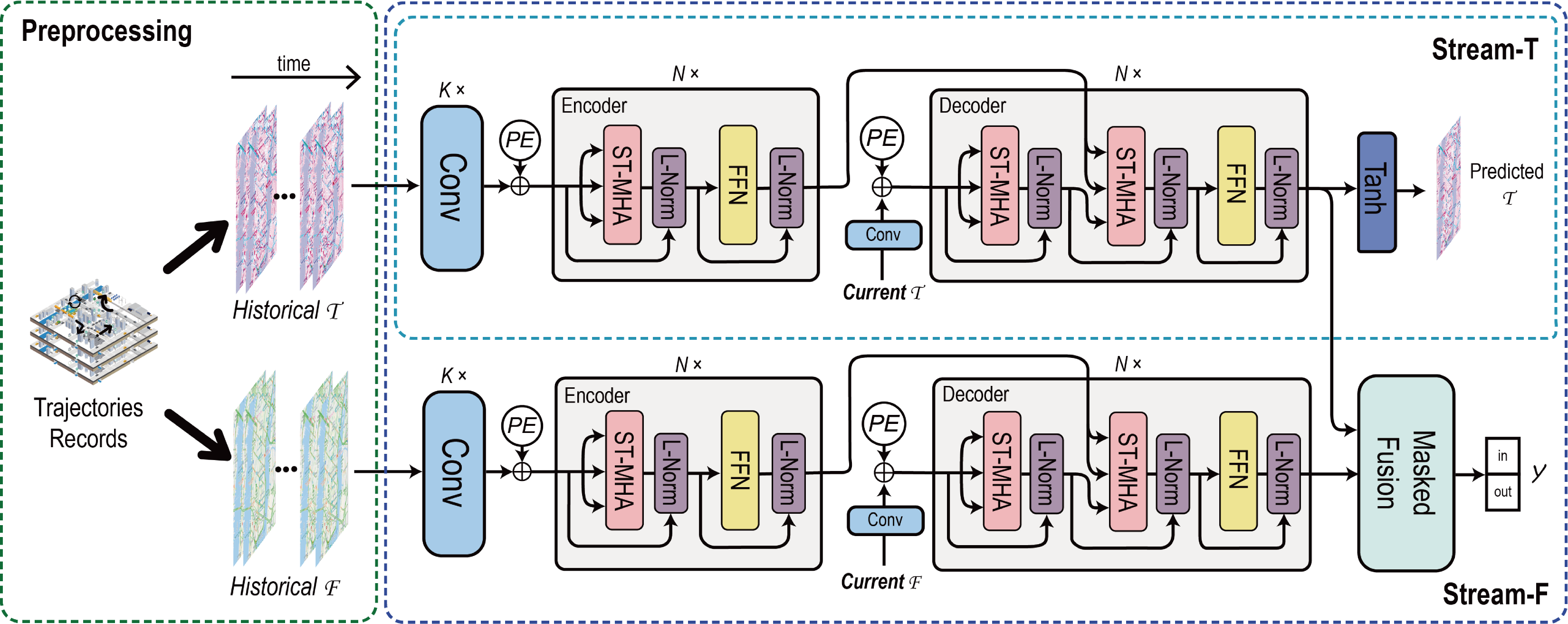
Figure 2 shows the architecture of ST-SAN, which consists of 2 streams of self-attention networks – Stream-T and Stream-F. Each of them contains a stack of convolutional layers, an encoder, and a decode. The Stream-T is trained independently on capturing features of transition before merging with Stream-F by a masked fusion mechanism. The detail of each component is described in the following subsections.
Encoder and Decoder
We employ the encoder-decoder architecture as in most competitive neural sequence transduction models [\citeauthoryearVaswani et al.2017]. Here, the encoder maps an inputs sequence of historical flow or transition data ( or ) to a sequence of continuous representations Z. Given Z and the current flow or transition data ( or ), the decoder then generates an output y as the predicted output of the next time interval.
The encoder contains a stack of N = 4 identical layers, whose sub-layers includes a spatial-temporal multi-head self-attention mechanism and a position-wise fully connected feed-forward network. We also employ the residual connection [\citeauthoryearHe et al.2015] and layer normalization [\citeauthoryearBa, Kiros, and Hinton2016] around each of the two sub-layers. To be specific, the output of each sub-layers is , where Sublayer(x) is the function implemented by the sub-layer itself. The dimension of outputs produced by all sub-layers is set to = 64, in order to facilitate the residual connections.
The decoder consists of a stack of N = 4 identical layers as well. Besides the two sub-layers in each encoder layer, an additional sub-layer is inserted to performs spatial-temporal multi-head attention over the output of the encoder stack. Also, residual connections followed by layer normalizations are implemented around each sub-layers.

Spatial-Temporal Self-Attention
Compared to ordinary self-attention mechanism adopted in language models, the feature space of the spatial-temporal self-attention mechanism has two more axes inserted to hold the domain of spatial map. As the computation of self-attention can be parallelized [\citeauthoryearVaswani et al.2017], an enlarged feature space does not result in longer training time.
In spatial-temporal self-attention, the scaled dot-product attention [\citeauthoryearVaswani et al.2017] is used as the attention kernel (Figure 3 (a)):
| (2) |
The inputs consist of queries, keys and values, as Q, K, V , where is the size of spatial maps and h, stand for sequence length and feature dimension. The transpose of K is performed between the last 2 axes where . Also, the matrix multiplication between Q, is over the last two axes. Then a multi-head attention is constructed upon the scaled dot-product attention:
| (3) | ||||
where are the learned projection parameter matrices and is the number of attention head. In this work, we employ u = 8 parallel attention layers, or heads. As the concepts of scaled dot-product attention and multi-head attention have been widely adopted in AI researches, here we exclude their comprehensive descriptions and refer readers to [\citeauthoryearVaswani et al.2017].
Local Convolution and Area of Interest
Before passing the spatial-temporal data into the spatial-temporal self-attention mechanism, they go through a stack of convolutional neural networks (CNN) with = 3 layers inside (Figure 2). The w types of flows will be projected to a representation space with dimension = 64, and the spatial dependencies are further interrelated via the CNN stack. Previous works have shown that when predicting the flow of , instead of measuring the whole spatial map, focusing on local dependencies is more helpful for the prediction [\citeauthoryearZhang, Zheng, and Qi2017b]. Therefore, we also adopt the idea of local convolution, which focuses on an area of interest (AoI) surrounding . Specifically, the historical flow input is sampled from all AoIs in historical spatial-temporal data. Similarly, when generating historical transition input , only the transitions between and the other nodes in the AoIs are sampled. In this work, we set a = b = 7.
The output of each layer in the CNN stack is computed as:
| (4) |
where is a slice of or , and is the convolutional result of on the p-th channel. is the weight of the p-th filter of convolution kernal , whose filter size is . All constitute a joint kernal , and the final output of each layer in the CNN stack is as:
| (5) |
where is or , and is the projected spatial-temporal representation of the input data. represent the slice-wise joint convolutional operation. We employ padding with the same value for each convolutional layer to maintain the same tensor shape.
Periodic Shifting and Sliding-Window Sampling
Previous work [\citeauthoryearYao et al.2019] demonstrated that the flows in periodic windows have strong similarities. As shown in Figure 4, the same periods of different days are more similar to each other than those in the previous periods on the same day. Besides, the pattern of flow will shift periodically. For example, the peak hours of traffic flow may vary from 16:30 to 18:00 on different days. Thus, we adopt sliding-window sampling to generate inputs of flow and transition from and to form . Specifically, is the concatenation of spatial matrices from the same periods of the previous = 7 days and the previous two-time intervals of the current day (area with red boundary in Figure 4). Then, data in the time interval before the future time is used as the current data fed in the decoder stack while the remained are used as input of the encoder stack.
Positional Encoding
Positional encoding is employed as the positional information is missed without the recurrent structures. Here, to encode the non-consecutive positional information, we add learned positional encodings to the output of the convolution stack. First, we represent the time information of as a one-hot vector , where g is the number of time intervals in one day. We use the first seven elements of to represent the day in a week and the last g elements to represent the index of time interval in that day. The positional encoding () of is as:
| (6) |
where are the learned parameters, and is the sigmoid function. Then the whole positional encoding matrix is formed and summed with before fed in the encoder and decoder stacks. The broadcast of to the same shape of is performed before the adding.

2-Stream Structure
Previous works demonstrate that transitions between nodes have significant impacts in flow prediction [\citeauthoryearYao et al.2018a]. Therefore, ST-SAN is designed as a 2-stream framework with two spatial-temporal self-attention networks (Stream-T, Stream-F) to measure flow and transition independently. We first train the Stream-T on predicting the transitions in AoI. Here the output of the Stream-T is as:
| (7) |
where . are learned parameters and is the output from the decoder stack.
Then, the trainable parameters of Stream-T will be locked and merged with Stream-F by a masked fusion mechanism to form the ST-SAN for further training. The independent training is necessary since we observe that the Stream-T will be ambiguously trained if only loss between the output and the true flow is calculated. Hence, independent training sets a more definite target for Stream-T, which enhances the measurement of transition. The experimental results also show the advantages of employing independent training.
Masked Fusion Mechanism
A masked fusion mechanism is proposed to merge the two streams and generate the final output. As shown in Figure 3 (b), the outputs of Stream-T () and Stream-F () are fed in a stack of = 2 hybrid convolutional layers, where its -th layer’s output is computed as:
| (8) | ||||
where are the convolutional kernels and learned bias. The function converts the transition features to a weight mask. Then the mask is applied on the convolutional result of to intensify the influence of more relative nodes. To be specific, if two nodes have many transitions between, consequently their connection and mutual influences should be stronger. Here, padding is not employed in the CNN layers.
After the output of the hybrid layer is flattened, the final output is then computed:
| (9) |
where is the flattened output.
The predicted outputs of all nodes {} constitute the predicted values of the whole spatial map (grid map) .
Loss
We use MSE loss function on both the training of Stream-T and the unified ST-SAN:
| (10) |
| (11) |
where are the ground truths of flows and AoI transitions of and and are the learnable parameters of Stream-T and ST-SAN.
| Model | Taxi-NYC | Bike-NYC | Mobile M | |||||||
|---|---|---|---|---|---|---|---|---|---|---|
| inflow | outflow | inflow | outflow | user number | ||||||
| RMSE | MAE | RMSE | MAE | RMSE | MAE | RMSE | MAE | RMSE | MAE | |
| HA | 90.19 | 50.10 | 109.36 | 65.91 | 30.25 | 20.35 | 29.63 | 19.96 | 421.39 | 273.18 |
| ARIMA | 33.54 | 18.62 | 40.70 | 23.61 | 17.14 | 10.83 | 18.03 | 11.28 | 194.92 | 150.95 |
| VAR | 48.04 | 23.21 | 128.67 | 29.84 | 27.37 | 14.29 | 27.67 | 15.09 | 254.37 | 157.71 |
| MLP | 27.13 | 16.91 | 32.93 | 20.80 | 25.77 | 32.57 | 15.92 | 19.85 | 130.01 | 106.44 |
| LSTM | 24.35 | 15.07 | 30.41 | 19.18 | 24.79 | 32.06 | 15.61 | 20.62 | 111.70 | 93.80 |
| GRU | 24.37 | 15.17 | 30.25 | 19.14 | 24.62 | 31.37 | 15.22 | 19.77 | 114.23 | 93.89 |
| ConvLSTM | 22.25 | 14.13 | 27.39 | 17.38 | 9.71 | 7.07 | 11.09 | 7.78 | 85.97 | 67.12 |
| ST-ResNet | 20.34 | 12.90 | 25.54 | 16.21 | 9.32 | 6.79 | 10.45 | 7.33 | 74.30 | 55.03 |
| DMVST-Net | 18.99 | 12.24 | 24.07 | 15.39 | 8.95 | 6.52 | 9.75 | 6.84 | 68.09 | 50.50 |
| STDN | 17.91 | 11.37 | 23.47 | 14.89 | 8.58 | 6.25 | 9.44 | 6.62 | 62.59 | 43.22 |
| ST-SAN | 16.39 | 10.63 | 22.94 | 13.48 | 7.82 | 5.68 | 9.02 | 6.17 | 57.13 | 40.20 |
Experiment
Datasets
We evaluate our model on three real-world datasets – Taxi-NYC, Bike-NYC, and Mobile M. Their details are showed in Table 2.
- •
Taxi-NYC and Bike-NYC: Taxi-NYC and Bike-NYC both contain 60 days of trip records. Each record includes the locations and times of the start and the end of a trip. We use the first 40 days as training data, and the remained 20 days as testing data.
- •
Mobile M: Mobile M includes 158,742,004 service records that contain the approximate locations of mobile phone users during the service periods. The whole 92-day dataset is split to 60 and 32 days for training and testing.
Evaluation Metric & Baselines
We measure the performance of different methods by two widely adopted metrics: (1) Rooted Mean Square Error (RMSE); (2) Mean Absolute Error (MAE).
| Datasets | Taxi-NYC | Bike-NYC | Modile M |
|---|---|---|---|
| Grid map size | |||
| Time interval | 30 mins | 30 mins | 15 mins |
| Time Span | 1/1/2016 - | 8/1/2016 - | 10/1/2018 - |
| 2/29/2016 | 9/29/2016 | 12/31/2018 | |
| Total records | 22,437,649 | 9,194,087 | 158,742,004 |
Baselines
- •
HA: Historical average.
- •
ARIMA: Auto-regressive integrated moving average model.
- •
VAR: Vector auto-regressive model.
- •
MLP: Multi-layer perceptron.
- •
LSTM: Long-Short-Term-Memory [\citeauthoryearHochreiter and Schmidhuber1997].
- •
GRU: Gated-Recurrent-Unit network [\citeauthoryearChung et al.2014].
- •
ConvLSTM: Convolutional LSTM [\citeauthoryearSHI et al.2015].
- •
ST-ResNet: Spatial-Temporal Residual Convolutional Network [\citeauthoryearZhang, Zheng, and Qi2017a].
- •
DMVST-Net: Deep Multi-View Spatial-Temporal Network[\citeauthoryearYao et al.2018b].
- •
STDN: Spatial-Temporal Dynamic Network [\citeauthoryearYao et al.2019].
Preprocessing
The grid sizes of Taxi-NYC, Bike-NYC, and Mobile M are , , and respectively. The length of the time interval is set as 30 minutes and 15 minutes, whereas the number of time interval in every day is 48 and 96. We randomly select 20% of data of training dataset for validation and the remained for training. We use Min-Max normalization to convert all traffic flow data to scale of [0, 1], and convert them back during the evaluation. We also filter out all regions with real flow volume less than ten in the evaluation, which is a common criterion used in flow prediction research area [\citeauthoryearZhang, Zheng, and Qi2017a].
Hyperparameters
In Taxi-NYC and Bike-NYC, = 2 types of flow – inflow and outflow, are processed. In Mobile M, only user number of each area is considered ( = 1). We set threshold m = 2 to filter out long-span transitions. The stack of convolutional layers contains = 3 layers of CNN, each of which includes = 64 filters with kernel size = . We set the dimension of Feed-Forward layer to 128 and the number of attention head to 8. The dropout rate is 0.1, and the epsilon offset in layer normalization is -1e6.
Optimizer
We used the Adam optimizer [\citeauthoryearKingma and Ba2014] with = 0.9, = 0.98 and . We adopted warm-up to adjust the learning rate:
| (12) |
where = 4000.
Results
We evaluated our methods and ten baselines on all three datasets and obtained the average results of each method after ten executions. Table 1 demonstrates the results of RMSE and MAE.
Noticeably, traditional statistic time-series prediction methods (HA, ARIMA, and VAR) are significantly less effective. It exposes the weakness of methods of exclusively considering the relation of historical statistic values and ignoring the complicated spatial-temporal dependency. For MLP, it barely learned the linear mapping from historical data to the predicted results, the spatial-temporal dependencies are insufficiently measured. LSTM and GRU achieved non-trivial improvement compared to MLP and traditional time-series methods given their effectiveness on modeling temporal dependency. Nonetheless, without a sophisticated mechanism to integrate spatial dependencies, their performance failed to improve further.
Deep-learning based methods showed their advantage of capturing complicated spatial-temporal dependencies. As shown in the comparison result, ST-SAN has outperformed the other deep learning frameworks. For ST-ResNet, despite it employs deep residual networks to capture spatial-temporal dependencies, the convolutional results are linearly merged, which overlooks the distinctive impacts of short-term and long-term temporal dependencies. ConvLSTM, DMVST-Net, and STDN showed the remarkable capability of modeling both the spatial and temporal dependencies. However, the LSTM employed limits their efficiencies on reaching long-term temporal dependencies. Besides, independent modeling of spatial and temporal dependencies also limits their capacity of capturing complicate spatial-temporal correlations. ST-SAN shows significant improvement compared to previous deep learning methods. In details, taking the prediction on Taxi-NYC data as an example, the RMSE is reduced by 9% for inflow prediction and 4% for outflow prediction.
Model Variants
Evaluation on the Effectiveness of Spatial-Temporal Self-Attention Mechanism
In this section, we empirically demonstrate the effectiveness of the spatial-temporal self-attention mechanism. There are three variants of the self-attention networks:
| Variants | RMSE/MAE | |
|---|---|---|
| inflow | outflow | |
| SAN | 22.38/13.98 | 28.17/16.44 |
| ST-SAN-S | 19.38/12.98 | 24.97/16.44 |
| ST-SAN-D | 16.73/10.91 | 23.34/14.07 |
| ST-SAN-D IT | 16.39/10.63 | 22.94/13.48 |
- •
SAN: Original self-attention network. The spatial maps are embedded into vectors by fully connected layers. Except for the input and output layers, SAN is identical to the Transformer.
- •
ST-SAN-S: Single-stream ST-SAN employing spatial-temporal self-attention network.
- •
ST-SAN-D: Dual-stream (2-stream) ST-SAN without independent training on Stream-T.
As shown in Table 3, ST-SAN-D outperforms other variants based on RMSE and MAE. SAN obtains poor performance as it merely employs the structure of Transformer ignoring the complicated spatial dependencies. ST-SAN-S applies the spatial-temporal self-attention mechanism, but the transition information between nodes is missed, which leads to the uniform measurement of influences of other nodes and overlooks their dynamic dependencies.
Evaluation on Effectiveness of Independent Training
To demonstrate the effectiveness of independent training on Stream-T, we evaluate the performance of 2 variants:
- •
ST-SAN-D
- •
ST-SAN-D IT: ST-SAN with independent training on Stream-T.
The results demonstrated in Table 3 show that ST-SAN-D MT achieves reasonable improvement compared to other variants. As mentioned above, if ST-SAN is only trained toward predicting flow, the target of Stream-T is ambiguous. Therefore, independent training of Stream-T reduces the ambiguity, leading to more accurate modeling of connectivity between nodes. Consequently, the final training on flow prediction task benefits from the pre-training.
Conclusion and Future Work
In this work, we present the spatial-temporal self-attention network. We introduce a spatial-temporal self-attention mechanism that simultaneously captures spatial and temporal dependencies while measuring long-term dependencies more efficiently. In addition, we proposed an independent training scheme to enhance the network’s ability to measure the connectivities of nodes. Experiment results demonstrate the significant improvement achieved by ST-SAN. In future work, we will focus on improving the performance of outflow prediction. During the experiment, we observed that ST-SAN achieved much fewer improvement on outflow prediction compared to inflow prediction. To find out the reason is one of the main tasks of our future works.
References
- [\citeauthoryearBa, Kiros, and Hinton2016] Ba, J. L.; Kiros, J. R.; and Hinton, G. E. 2016. Layer normalization.
- [\citeauthoryearChung et al.2014] Chung, J.; Gülçehre, Ç.; Cho, K.; and Bengio, Y. 2014. Empirical evaluation of gated recurrent neural networks on sequence modeling. CoRR abs/1412.3555.
- [\citeauthoryearCui, Ke, and Wang2016] Cui, Z.; Ke, R.; and Wang, Y. 2016. Deep bidirectional and unidirectional LSTM recurrent neural network for network-wide traffic speed prediction. CoRR abs/1801.02143.
- [\citeauthoryearDevlin et al.2018] Devlin, J.; Chang, M.; Lee, K.; and Toutanova, K. 2018. BERT: pre-training of deep bidirectional transformers for language understanding. CoRR abs/1810.04805.
- [\citeauthoryearHe et al.2015] He, K.; Zhang, X.; Ren, S.; and Sun, J. 2015. Deep residual learning for image recognition. CoRR abs/1512.03385.
- [\citeauthoryearHochreiter and Schmidhuber1997] Hochreiter, S., and Schmidhuber, J. 1997. Long short-term memory. Neural Computation 9(8):1735–1780.
- [\citeauthoryearKe et al.2017] Ke, J.; Zheng, H.; Yang, H.; and Chen, X. 2017. Short-term forecasting of passenger demand under on-demand ride services: A spatio-temporal deep learning approach. CoRR abs/1706.06279.
- [\citeauthoryearKingma and Ba2014] Kingma, D., and Ba, J. 2014. Adam: A method for stochastic optimization. International Conference on Learning Representations.
- [\citeauthoryearLi et al.2012] Li, X.; Pan, G.; Wu, Z.; Qi, G.; Li, S.; Zhang, D.; Zhang, W.; and Wang, Z. 2012. Prediction of urban human mobility using large-scale taxi traces and its applications. Frontiers of Computer Science 6(1):111–121.
- [\citeauthoryearMoreira-Matias et al.2013] Moreira-Matias, L.; Gama, J.; Ferreira, M.; Moreira, J.; and Damas, L. 2013. Predicting taxi-passenger demand using streaming data. IEEE Transactions on Intelligent Transportation Systems 14:1393–1402.
- [\citeauthoryearRadford et al.2019] Radford, A.; Wu, J.; Child, R.; Luan, D.; Amodei, D.; and Sutskever, I. 2019. Language models are unsupervised multitask learners.
- [\citeauthoryearRavi Chandra and Al-Deek2009] Ravi Chandra, S., and Al-Deek, H. 2009. Predictions of freeway traffic speeds and volumes using vector autoregressive models. Journal of Intelligent Transportation Systems 13:53–72.
- [\citeauthoryearShekhar and Williams2008] Shekhar, S., and Williams, B. 2008. Adaptive seasonal time series models for forecasting short-term traffic flow. Transportation Research Record 2024:116–125.
- [\citeauthoryearSHI et al.2015] SHI, X.; Chen, Z.; Wang, H.; Yeung, D.-Y.; Wong, W.-k.; and WOO, W.-c. 2015. Convolutional lstm network: A machine learning approach for precipitation nowcasting. In Cortes, C.; Lawrence, N. D.; Lee, D. D.; Sugiyama, M.; and Garnett, R., eds., Advances in Neural Information Processing Systems 28. Curran Associates, Inc. 802–810.
- [\citeauthoryearVaswani et al.2017] Vaswani, A.; Shazeer, N.; Parmar, N.; Uszkoreit, J.; Jones, L.; Gomez, A. N.; Kaiser, L. u.; and Polosukhin, I. 2017. Attention is all you need. In Guyon, I.; Luxburg, U. V.; Bengio, S.; Wallach, H.; Fergus, R.; Vishwanathan, S.; and Garnett, R., eds., Advances in Neural Information Processing Systems 30. Curran Associates, Inc. 5998–6008.
- [\citeauthoryearWu and Tan2016] Wu, Y., and Tan, H. 2016. Short-term traffic flow forecasting with spatial-temporal correlation in a hybrid deep learning framework. CoRR abs/1612.01022.
- [\citeauthoryearYang et al.2019] Yang, Z.; Dai, Z.; Yang, Y.; Carbonell, J. G.; Salakhutdinov, R.; and Le, Q. V. 2019. Xlnet: Generalized autoregressive pretraining for language understanding. CoRR abs/1906.08237.
- [\citeauthoryearYao et al.2018a] Yao, H.; Wu, F.; Ke, J.; Tang, X.; Jia, Y.; Lu, S.; Gong, P.; Li, Z.; Ye, J.; and Chuxing, D. 2018a. Deep multi-view spatial-temporal network for taxi demand prediction. In 32nd AAAI Conference on Artificial Intelligence, AAAI 2018, 32nd AAAI Conference on Artificial Intelligence, AAAI 2018, 2588–2595. AAAI press.
- [\citeauthoryearYao et al.2018b] Yao, H.; Wu, F.; Ke, J.; Tang, X.; Jia, Y.; Lu, S.; Gong, P.; Ye, J.; and Li, Z. 2018b. Deep multi-view spatial-temporal network for taxi demand prediction. CoRR abs/1802.08714.
- [\citeauthoryearYao et al.2019] Yao, H.; Tang, X.; Wei, H.; Zheng, G.; and Yu, Y. 2019. Revisiting spatial-temporal similarity: A deep learning framework for traffic prediction. AAAI’19 227.
- [\citeauthoryearZhang et al.2016] Zhang, J.; Zheng, Y.; Qi, D.; Li, R.; and Yi, X. 2016. Dnn-based prediction model for spatio-temporal data. In Proceedings of the 24th ACM SIGSPATIAL International Conference on Advances in Geographic Information Systems, SIGSPACIAL ’16, 92:1–92:4. New York, NY, USA: ACM.
- [\citeauthoryearZhang et al.2019] Zhang, J.; Zheng, Y.; Sun, J.; and Qi, D. 2019. Flow prediction in spatio-temporal networks based on multitask deep learning. IEEE Transactions on Knowledge and Data Engineering 1–1.
- [\citeauthoryearZhang, Zheng, and Qi2017a] Zhang, J.; Zheng, Y.; and Qi, D. 2017a. Deep spatio-temporal residual networks for citywide crowd flows prediction. In Proceedings of the Thirty-First AAAI Conference on Artificial Intelligence, AAAI’17, 1655–1661. AAAI Press.
- [\citeauthoryearZhang, Zheng, and Qi2017b] Zhang, J.; Zheng, Y.; and Qi, D. 2017b. Deep spatio-temporal residual networks for citywide crowd flows prediction.
- [\citeauthoryearZhou et al.2018] Zhou, X.; Shen, Y.; Zhu, Y.; and Huang, L. 2018. Predicting multi-step citywide passenger demands using attention-based neural networks. In Proceedings of the Eleventh ACM International Conference on Web Search and Data Mining, WSDM ’18, 736–744. New York, NY, USA: ACM.