The location of the last stable orbit in Kerr spacetime

Hereafter we shall be concerned with bound orbits about a Kerr black hole. For such orbits the radial motion is confined within the region $r_{p}\leq r\leq r_{a}$, where $r_{p}$ and $r_{a}$ are the minimum (pericenter) and maximum (apocenter) radii obtained during the orbital motion, respectively. Similarly, the polar motion is confined within the region $\theta_{\text{min}}\leq\theta\leq\theta_{\text{max}}=\pi-\theta_{\text{min}}$. An orbit in the equatorial plane has $\theta=\theta_{\text{min}}=\pi/2$.

There are infinitely many ways to parametrize geodesic motion in Kerr spacetime. For bound orbits it is convenient to change from the set $(\mathcal{E},\mathcal{L}_{z},\mathcal{Q})$ to a Keplerian-inspired choice. One such choice for the radial motion is the quasi-Keplerian parameterization,

where $p$ is the dimensionless semi-latus rectum, $0\leq e<1$ is the orbital eccentricity, and $\psi$ is a monotonically increasing radial phase parameter. The minimum (pericenter) and maximum (apocenter) radii occur at

which can be inverted to give

Using the parameterization of Eq. (12) will avoid the issue of sign flipping at turning points, since the radial phase $\psi$ is monotonically increasing. Further, one can show that this parameterization analytically cancels the zeroes in $R(r)$ at $r_{p}$ and $r_{a}$, thus making the ODE satisfy the Lipschitz condition.

A similar approach works for the polar angle. Defining $z=\cos\theta$, we can write

where $z_{m}=\cos\theta_{\text{min}}$, so $\pm z_{m}$ are the maximum/minimum values achieved by $\cos\theta$, and $\chi$ is a monotonically increasing phase angle. This parameterization similarly solves the sign choice and Lipschitz continuity issues.

One drawback of using $z_{m}$ as an “inclination” parameter is that it does not distinguish between prograde and retrograde orbits. This distinction must be implemented by making $a<0$ for retrograde orbits. Besides $z_{m}$, there are many common parameterizations for the inclination angle in the literature. Because of the plethora of inclination parameterizations in the literature care must be taken when comparing results between different works. In this work we primarily use

This has the nice property that the orbital parameters smoothly vary from prograde equatorial motion ($x=1$) to retrograde equatorial motion ($x=-1$), without having to flip the sign of $a$. The relationship between $\theta_{\text{min}}$ and $\theta_{\text{inc}}$ is diagrammed in Fig. 1. The parameters $x$ and $z_{m}$ satisfy the polynomial relationship $x^{2}+z_{m}^{2}=1$, which is significant in that any polynomial results developed with $x^{2}$ will also be polynomial in $z_{m}^{2}$. Another commonly used inclination angle is $\cos\iota=\mathcal{L}_{z}/\sqrt{\mathcal{L}_{z}^{2}+\mathcal{Q}}$. Using $\cos\iota$ or $\sin\iota$ also turns out to yield polynomial relations below.

When parameterizing an orbit by $(p,e,x)$, it is crucial to know how to convert back and forth between these parameters and the constants $(\mathcal{E},\mathcal{L}_{z},\mathcal{Q})$. The bijective relationship Warburton et al. 2013 between $(p,e,x)\leftrightarrow(\mathcal{E},\mathcal{L}_{z},\mathcal{Q})$ is well known for bound orbits in Schwarzschild spacetime Cutler et al. 1994 as well as equatorial orbits Glampedakis and Kennefick 2002, spherical orbits Hughes 2000, and generic orbits in Kerr spacetime Schmidt 2002. Unfortunately, not all of $(p,e,x)$ space maps to stable bound orbits, or even to physically realizable motion. Finding the separatrix between the stable and plunging orbits is the subject of the remainder of this paper.

Certain classes of orbital configurations are simpler to analyze than others. These special classes of orbits are as follows:

1. 1.

   Equatorial orbits. These lie in the equatorial plane ($\theta=\pi/2$) and have $|x|=1$.

2. 2.

   Polar orbits. These orbits have $x=0$ which corresponds to $\mathcal{L}_{z}=0$. They intersect the axis of symmetry of the black hole.

3. 3.

   Spherical orbits. These orbits have $e=0$ and ${|x|\neq 1}$. These orbits have fixed Boyer-Lindquist radius and librate in the polar direction.

4. 4.

   Circular orbits. These orbits have $e=0$ and $|x|=1$. These orbits lie in the equatorial plane and have a fixed Boyer-Lindquist radius.

5. 5.

   Parabolic trajectories. These have $e=1$ and ${\mathcal{E}=1}$, sending apocenter to infinity, so are marginally bound and technically not orbits.

If an orbital configuration does not fall into any of the above categories we refer to it as a ‘generic’ orbit.

Bound radial motion occurs between two roots of the radial polynomial $R(r)$. The four roots are traditionally labeled as $r_{1}\geq r_{2}\geq r_{3}\geq r_{4}$ (when they are all real), in the factorization

The signs above are chosen since bound motion happens in the range $r_{p}=r_{2}\leq r\leq r_{1}=r_{a}$, and $\mathcal{E}^{2}<1$ for bound motion.

When $r_{2}>r_{3}$, there is a simple root, $R(r_{2})=0$ and $R^{\prime}(r_{2})\neq 0$, and thus a ‘restoring force’ to keep the particle from plunging. By contrast, if we have a root with higher multiplicity, $r_{2}=r_{3}$ (or $r_{1}=r_{2}=r_{3}$ for circular orbits), then the derivative of the radial polynomial vanishes, $R^{\prime}(r_{2})=0$. This means there is no ‘restoring force’ at pericenter, so an infinitesimal perturbation can make the orbit plunge.

This gives the condition for the separatrix in parameter space: the set of parameters where these roots degenerate, solving the equation $r_{2}(p,e,x)=r_{3}(p,e,x)$.

The root $r_{2}=pM/(1+e)$ is a simple function of $p$ and $e$. The root $r_{3}$ is much more complicated, though it is possible to express it in terms of nested radicals (this earlier method is described in Sec. V.1). We however pursue an approach which yields the separatrix polynomial $S(a,p,e,x)$, where the separatrix lies along roots of the polynomial equation $0=S(a,p,e,x)$.

To find the separatrix polynomial, we start by posing the location of the separatrix as the simultaneous solutions of the following system of equations:

It is important to note here that every equation in system (18) is a rational polynomial in all the following indeterminates: $(a,p,e,z_{m},\mathcal{E},\mathcal{L}_{z},\mathcal{Q})$. Since $\Theta$ is a function only of the square $z_{m}^{2}=1-x^{2}$, this system is still a system of rational polynomials in $x$ instead of $z_{m}$. The same property is true if we use $\sin\iota$ or $\cos\iota$ instead of $z_{m}$. We overload the symbol $\Theta$ to mean the appropriate function of each variable, so we write $\Theta(x)$.

Now if we avoid vanishing denominators (the point is said to be in general position), we can clear denominators to form a system of polynomials in these indeterminates. This system is

The simultaneous solution of a system of polynomial equations forms an algebraic variety, the fundamental object of algebraic geometry. Even before modern algebraic geometry, in classical elimination theory it was known that one could eliminate indeterminates from such a system at the expense of raising the polynomial degree of the remaining system. The classic method is based on generalizations and improvements to Dixon’s resultant Dixon 1909 (see e.g. Kapur et al. 1994). The more modern algebraic geometry approach would construct a Gröbner basis for the ideal of the ring of polynomials vanishing on the variety defined by system (19).

The upshot is that with these four equations, we can eliminate the three indeterminates $(\mathcal{E},\mathcal{L}_{z},\mathcal{Q})$, and be left with the single separatrix polynomial $S(a,p,e,x)$. As noted earlier, if one desires, the same approach works in terms of $z_{m},\cos\iota$, or $\sin\iota$ instead of $x$. This can be accomplished with a computer algebra system such as Mathematica with a bit of guidance. The separatrix polynomial is 12${}^{\text{th}}$ degree in $p,a,e$ and 4${}^{\text{th}}$ degree in $x^{2}$, so is a bit cumbersome. After clearing some unwanted denominators introduced by elimination, we present $S$ as

where the $S_{n}$ are polynomials in $a$, $e$, and $x^{2}$ that we tabulate in App. A. We make the algebraic derivation and machine-readable expressions available in the companion Mathematica notebook distributed with this article Sep.

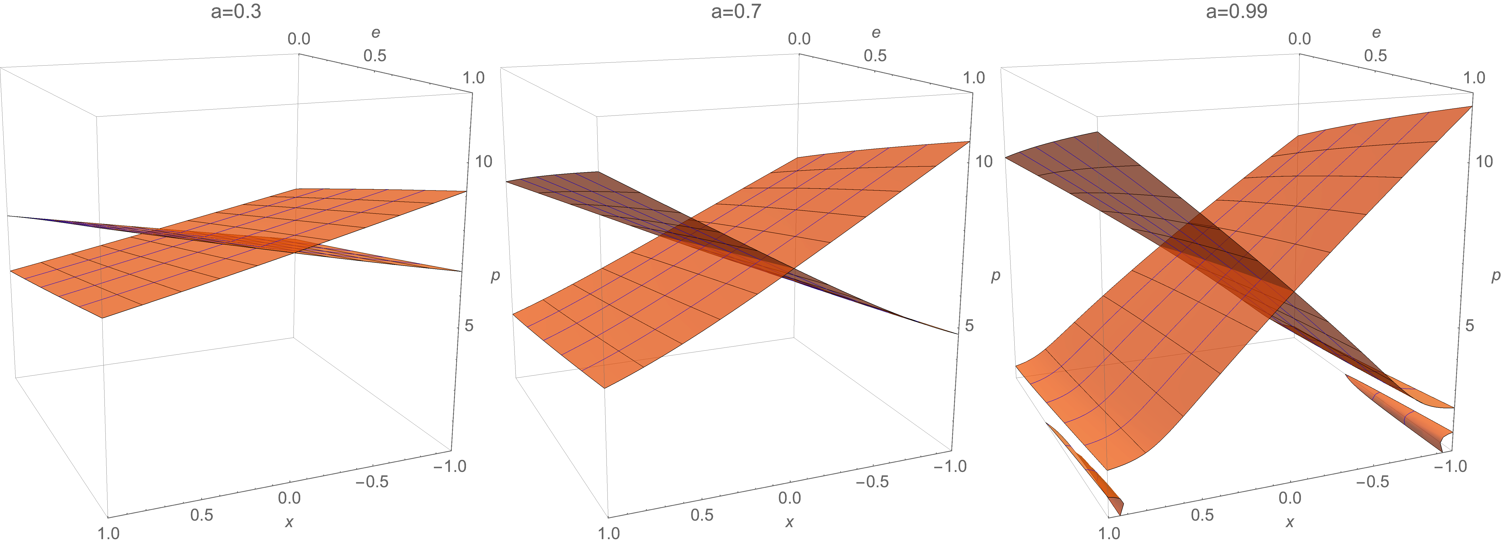
Figure 2 gives an overview of the set of points satisfying $S=0$. The polynomial $S$ is even in $x$, which is reflected in the reflection symmetry in the figure. Correspondingly, the polynomial is satisfied at both the prograde and retrograde values of $p$ associated to a particular $x^{2}$.

The separatrix itself is just one of the “leaves” of the solutions seen in Fig. 2, specifically the one for which $p$ decreases with increasing $x$, as prograde orbits exist closer than retrograde ones. Note also that there are additional unphysical solutions which appear at smaller $p$ at high spin and eccentricity – more on this in Sec. IV.2.1.

One might hope that the separatrix polynomial could be factorized into a lower-degree polynomial for each “leaf” of the solution set. Taking a more global view shows that this is impossible. In Fig. 3 we show a view of the affine variety (i.e. the set of solutions) that extends to unphysical values of $e<0$. There we see that at $e=-1$, the prograde and retrograde “leaves” are smoothly connected, so they are part of the same algebraic set.

The high degree of the separatrix polynomial makes finding analytic solutions for generic orbits unfeasible. Instead we now concentrate on analytic results for interesting limiting cases. We then present techniques for numerically computing the location of the separatrix for generic orbits.

As Schwarzschild spacetime is spherically symmetric, the separatrix must be independent of $x$. If we set $a=0$, we get the enormous simplification,

Thus we see that the Schwarzschild separatrix lies at $p_{\text{sep}}^{\text{Schw}}=6+2e$ Cutler et al. 1994.

Equatorial orbits have $x^{2}=1$, with the sign encoding prograde/retrograde motion. This corresponds to $\mathcal{Q}=0$ and $\sin\iota=0$. In this case we also get a significant factorization,

where the nontrivial quartic polynomial is

This is the same as Eq. (B7) in O’Shaughnessy 2003 which is itself a simplified form of Eq. (23) in Glampedakis and Kennefick 2002. As Eq. (23) is quartic in $p$, there is an explicit solution by radicals for $p_{\text{sep}}^{\pm\text{equat}}(a,e)$.

Because of monotonicity, the global extrema are at $a=1,x=\pm 1$. Along the extremal spin limit $a=1$, the quartic is

The global minimum is at $a=1,e=0,x=+1$, with value $p_{\text{sep}}^{\text{min}}=1$. The global maximum is at $a=1,e=1,x=-1$, with value $p_{\text{sep}}^{\text{max}}=6+4\sqrt{2}\approx 11.66$. These two extremes bracket all values for physical solutions of the separatrix,

In the equatorial plane the separatrix is a one dimensional curve in the $(p,e)$ parameter space. A parameterization for this curve can be found by noting the connection between the separatrix and the unstable ‘whirl’ radius, $r_{u}=p/(1+e)$ of a homoclinic orbit Levin and Perez-Giz 2009. This radius varies in the range $r_{\text{ibco}}\leq r_{u}\leq r_{\text{isco}}$. The second inequality implies that $r_{u}(r_{u}-2)a+a^{3}\geq 0$. Simultaneously solving the set of equations $\{S_{\text{equat}}=0,r_{u}=p/(1+e)\}$ with the above constraint gives

These equations agree with the results in Ref. Levin and Perez-Giz 2009.

Polar orbits have $x=0$, $\sin\iota=1$, which corresponds to $\mathcal{L}_{z}=0$. Recall that the full separatrix polynomial $S(p,e,x)$ is only a function of $x^{2}$ and thus even in $x$. We also know that the function $p_{\text{sep}}{}(x)$ is monotonic in $x$, with $p_{\text{sep}}{}$ being smaller for prograde (positive) and larger for retrograde (negative) values of $x$. Therefore as $x$ goes through 0, the physically relevant sheet of the solution set is crossing through the polar value $p_{\text{sep}}^{\text{pol}}$, in a simple root. But since $S$ depends only on $x^{2}$, the unphysical sheet is simply the reflection of the physical one with $x\to-x$. Thus there is a degeneracy at $x=0$, and further the polynomial factors as a square of a sextic. That is,

where the sextic is

From monotonicity, the minima and maxima of the polar separatrix occur respectively at $(a=1,e=0)$ and $(a=0,e=1)$. That is, for arbitrary $a$ and $e$, the polar separatrix always lies in this interval,

with equality only at the appropriate corners of the unit square in $(a,e)$ space.

When $a=0$, we have to recover Eq. (21), and indeed here we get $S_{\text{pol}}(a=0)=p^{5}(p-6-2e)$, again leading to $p_{\text{sep}}^{\text{Schw}}=6+2e$. Thus the global maximum for the polar separatrix is $p_{\text{sep}}^{\text{pol}}(0,1)=8$.

For the extremal limit $a=1$ there is no major simplification. But at the endpoints $e=0$ and $e=1$ there is, respectively,

From these we can find the real nontrivial roots of the separatrix polynomial at these corners of the unit square,

Thus the global minimum for the polar separatrix is $p_{\text{sep}}^{\text{pol}}(1,0)\approx 5.27$.

Specializing to spherical orbits entails setting $e=0$. Unfortunately the separatrix polynomial does not factor further at $e=0$. This polynomial, $S(e=0)$, agrees with one previously presented in Appendix A of Ref. Stone et al. 2013, based on the homoclinic orbit approach of Ref. Levin and Perez-Giz 2009.

Of course we can take further special cases where it does factor. For example, the equatorial circular separatrix polynomial is

The quartic can be solved by radicals, and the two physical solutions (prograde and retrograde) are the classic result of the equatorial ISCO given by Bardeen, Press, and Teukolsky Bardeen et al. 1972.

Another special case of interest is spherical orbits around an extremal black hole. Here we get the factorization

where the ninth degree factor is

where $z_{m}^{2}=1-x^{2}$. This polynomial may be described as “anti-reciprocal” in two indeterminates, in the sense that $S_{\text{sph., ext.}}(p,z_{m})=-p^{9}z_{m}^{8}S_{\text{sph., ext.}}(p^{-1},z_{m}^{-1})$.

Here we see an interesting phenomenon. For most values of $x$, one root that varies smoothly with $x$ is the physical root $p_{\text{sep}}^{\text{sph. ext.}}(x)$. But, this root crosses $p=1$ linearly at some critical value $x_{\text{kink}}^{\text{sph. ext.}}$. Above this value of $x$, the root $p=1$ becomes the physically relevant root, and this leads to a kink in the graph of $p_{\text{sep}}^{\text{sph. ext.}}(x)$. We find the inclination where the nonic also has a root at $p=1$ by setting $p$ to 1, leaving us to solve the polynomial $0=8x^{2}(x^{2}-2)(x^{4}+4x^{2}-4)$. We find the location of the kink is

Ref. Compère and Druart 2020 independently derived this result at the same time as this work. From Eq. (46) when $a=1$ and $x\geq x_{\text{kink}}^{\text{sph. ext.}}$, the ISSO is at $p=1$. This kink behavior can be seen in Fig. 5.

Parabolic encounters are astrophysically interesting for modeling tidal disruptions of ordinary stars around supermassive black holes Evans and Kochanek 1989; Stone et al. 2019; Hayasaki et al. 2018. They are also interesting as potential sources of gravitational wave bursts Berry and Gair 2013; Hopper and Cardoso 2018. A parabolic encounter has $e=1$, which sends the apocenter $r_{1}$ to infinity while $r_{2}=p/2$ remains finite. Notice that sending one root of $R(r)$ to infinity depresses the quartic to a cubic, which happens when $\mathcal{E}=1$.

Parabolic trajectories are technically not bound orbits. They are another type of parameter space separatrix, between eccentric (bound) and hyperbolic (unbound) trajectories. The set of all parabolic orbits also connects to the separatrix between bound and plunging orbits which we are analyzing in this paper, simply by restricting to $e=1$ in $S(a,p,e,x)$. This reflects an interesting phase space geometry which is beyond the scope of this work.

The separatrix polynomial also factorizes at $e=1$,

where the nontrivial factor is

Besides the $p$ degree being lowered, $S_{\text{para}}$ is only quadratic in $x^{2}$, meaning it is straightforward to give an explicit parametric description of the surface. Before doing so, we will further specialize to equatorial parabolic encounters to find the $p$ extrema of this slice through the separatrix. Setting $x=1$, we have the further simplification

Besides the unphysical roots at $p=0$, there are two additional quadratic factors which can be solved directly. The roots of physical interest give the extrema of the parabolic separatrix as a function of $a$,

The plus signs are taken for retrograde (larger $p$), and the minus signs are taken for prograde (smaller $p$).

To find the parametric description of the parabolic separatrix, match coefficients $(A,B,C)$ in $S_{\text{para}}=Ax^{4}+Bx^{2}+C$, then solve for $x^{2}$ in $0=S_{\text{para}}$,

where the discriminant is $D=2^{13}a^{4}p^{7}[4a^{2}+p(p-4)]^{2}$. If one takes the upper sign in Eq. (51), the values of $x_{\text{para}}^{2}$ are always greater than 1 and thus unphysical; therefore take the minus sign in Eq. (51). The parameter $p$ lies in the domain $p_{\text{para}}^{-}(a)\leq p\leq p_{\text{para}}^{+}(a)$, and the image $x_{\text{para}}^{2}(a,p)$ covers $[0,1]$ on this domain.

Given a set of geodesic parameters, determining if an orbit is stable is straightforward. Stable orbits have $r_{2}-r_{3}>0$, when both are real, and these roots are easily evaluated as follows. First, $(\mathcal{E},\mathcal{L}_{z},\mathcal{Q})$ can be expressed explicitly in terms of $(p,e,x)$ by following the procedure detailed in Appendix B of Schmidt Schmidt 2002. These analytic expressions involve nested radicals, and thus may become complex. Next we follow Fujita and Hikida Fujita and Hikida 2009 to find $r_{3}$ and $r_{4}$. Depress the quartic $R(r)$ by the known quadratic factor $(1-\mathcal{E}^{2})(r_{1}-r)(r-r_{2})$. This leaves the quadratic $(r-r_{3})(r-r_{4})$ which is solved explicitly for $r_{3}$ and $r_{4}$, again in terms of nested radicals, so $r_{3}$ and $r_{4}$ may also become complex.

Finding the precise location of the separatrix in a robust and computationally efficient way is more challenging. This is because, as mentioned above, in some regions of the parameter space $r_{2}-r_{3}$ becomes complex. This causes, e.g., a Newton-Raphson root finding scheme to fail – see Fig. 6 and, e.g., Appendix A of Sundararajan 2008. These challenging regions of the parameter space occur for high spin, near prograde equatorial orbits.

The problems mentioned above occur when the root finder steps over the separatrix to a value of $p<p_{\text{sep}}{}$ and the algorithm is unsure how to proceed because the function it is evaluating has become complex. One way to avoid this is to use a bisection-like method to seek the root strictly from above. In this method you pick an initial value of $p$ large enough to ensure $p>p_{\text{sep}}{}$, check if $r_{2}>r_{3}$ and if so decrease $p$ by some small amount $\Delta p_{\text{sep}}{}$. This is repeated until $r_{3}$ becomes complex at which point the previous value of $p$ is returned to and now $\Delta p_{\text{sep}}{}$ is halved and the process repeats. As this is a bisection-like method it is robust but does not converge quickly.

A robust approach that can use rapidly convergent numerical root finding was introduced into the Black Hole Perturbation Toolkit BHP in 2018 by one of us. This used an extension of the method of Ref. Levin and Perez-Giz 2009 from equatorial to generic orbits. We give the equations for this extension in Appendix D. Recently Ref. Rana and Mangalam 2019 published equations for a similar extension. In this approach one picks values for $e_{\text{sep}}{},x_{\text{sep}}{}$ and then root finds for an unstable circular orbit radius, $r_{u}$, in the range $r_{\text{ibso}}\leq r_{u}$. With $r_{u}$ strictly bounded below the method is robust and rapidly convergent numerical root finding techniques, like a Newton-Raphson method, can be employed. The downside to this method is that first $r_{\text{ibso}}$ must be found and this adds to the computational overhead.

We now discuss new approaches which are faster and guaranteed to find $p_{\text{sep}}{}$.

From the fundamental theorem of algebra, $S$ has 12 complex roots for $p$, and several methods exist to find all roots simultaneously. One standard “black-box” approach Press et al. 2007 is the method of Jenkins and Traub. There exists both a general version for polynomials with complex coefficients, and a more adapted algorithm for polynomials with real coefficients Jenkins and Traub 1970.

Another popular algorithm is the Aberth method Aberth 1973, which converges cubically to simple roots, but only exists in a complex form. If one were to initiate the Aberth method with purely real guesses for a real polynomial, the iteration scheme would never push the guesses into the complex plane, and would thus fail to find complex roots. Therefore it is important to start with complex guesses, though this means that all roots will acquire some imaginary part, even if the root is exactly on the real axis. Therefore using the Aberth method (or the complex version of the Jenkins-Traub method) requires testing roots $p_{i}$ for realness via $|\text{Im}[p_{i}]|\leq\epsilon$ with some arbitrary choice of $\epsilon>0$.

Such black-box global root-finding methods are implemented in most computer algebra systems and numerical libraries. For example, in Mathematica, the command NRoots[] implements both the Jenkins-Traub and Aberth methods.

For special values such as $x=0$, $x^{2}=1$, or $e=0$, one should use the appropriate simplified polynomial. Here we give the generic algorithm, for general points:

1. 1.

   Find all complex roots $p_{i}$, and select the real roots as those that satisfy $|\text{Im}[p_{i}]|\leq\epsilon$ with some $\epsilon>0$ determined by the required precision.

2. 2.

   If $x<0$, the orbit is retrograde and thus the desired root is the largest real root.

3. 3.

   If $x>0$, the orbit is prograde and thus the desired root is the second largest real root.

For polynomials with real coefficients, it is possible to bound the number of real roots and to isolate each real root into an interval of the real line, with black-box “real-root isolation” algorithms. At their most basic, these algorithms arise from Descartes’ rule of signs Descartes 1637, with improvement due to Sturm’s theorem Basu et al. 2013. Using real-root isolation, one is guaranteed to find brackets for all the simple real roots of $S(p)$ automatically. Such algorithms are implemented in several computer algebra systems, for example in the sage module sage.rings.polynomial.real_roots, or in the Mathematica commands RootIntervals[] or NSolve[…,Reals].

For special values such as $x=0$, $x^{2}=1$, or $e=0$, the separatrix polynomial is not square-free, and one should instead focus on solving the nontrivial factor such as $S_{\text{pol}}$. Here we give the generic algorithm, for general points:

1. 1.

   Find isolating intervals for all roots of $S(p)$ in the admissible physical range, $1\leq p\leq 6+4\sqrt{2}\approx 11.66$.

2. 2.

   If $x<0$, the orbit is retrograde and thus the desired root is the largest real root.

3. 3.

   If $x>0$, the orbit is prograde and thus the desired root is the second largest real root.

Rather than relying on a black box algorithm to find isolating intervals for real roots, we can analytically find them, using all the limiting cases presented in Sec. IV. The method we describe here is also the fastest and most robust, and the one that is implemented in the Black Hole Perturbation Toolkit BHP.

First note that we have the brackets,

where $\pm$equat refer to the prograde/retrograde equatorial orbits. These serve as brackets, if we know the values of the polar and equatorial separatrices. Those values are found via their own bracketed root-finding. The algorithm proceeds as follows, given some inputs $a,e,x$:

1. 1.

   In all cases one needs to find $p_{\text{sep}}^{\text{pol}}(a,e)$, by polishing the single simple root of the sextic $S_{\text{pol}}(p)$ given in Eq. (37), within the bracket

   $\displaystyle 1+\sqrt{3}+\sqrt{3+2\sqrt{3}}\leq p_{\text{sep}}^{\text{pol}}(a,e)\leq 8\,.$

   (54)

2. 2.

   If $x=0$, the orbit is polar and the separatrix has been found. Otherwise:

   1. (a)

      If $x>0$, find $p_{\text{sep}}^{+\text{equat}}(a,e)$, by polishing the single simple root of Eq. (23) within the bracket

      $\displaystyle 1+e$

      $\displaystyle\leq p_{\text{sep}}^{+\text{equat}}(a,e)\leq 6+2e\,.$

      (55)

      Now with $p_{\text{sep}}^{+\text{equat}}(a,e)$ and $p_{\text{sep}}^{\text{pol}}(a,e)$ in hand, polish the single simple root of the full 12${}^{\text{th}}$ degree $S(p)$ within the bracket Eq. (52).

   2. (b)

      If $x<0$, one can omit finding $p_{\text{sep}}^{-\text{equat}}(a,e)$, since there is only ever one root of the separatrix polynomial between $p_{\text{sep}}^{\text{pol}}(a,e)$ and the maximum possible value of the separatrix (discussed in Sec. IV.2), $p_{\text{sep}}^{\text{max}}=6+4\sqrt{2}\approx 11.66$. Therefore polish the single simple root of the full 12${}^{\text{th}}$ degree $S(p)$ within the bracket $p_{\text{sep}}^{\text{pol}}(a,e)\leq p_{\text{sep}}{}(a,e,x)\leq 12$.

The algorithm presented above to compute the separatrix is implemented in the KerrGeodesics Mathematica package of the Black Hole Perturbation Toolkit BHP. It can be accessed with a function called KerrGeoSeparatrix[a,e,x]. This algorithm replaced the slower algorithm outlined in Appendix D. The new method takes ~1ms to calculate the location of the separatrix to machine precision.¹¹ 1 This is measured on a 2.5GHz Macbook Pro laptop using Mathematica 12. This is roughly 45 times faster than the previous implementation which relied on multiple root finding steps.

In addition to numerically finding $p_{\text{sep}}{}$ the KerrGeoSeparatrix[a,e,x] function will also return the closed form analytic results for the special cases presented in Sec. IV.

References

- McClintock et al. (2011) J. E. McClintock, R. Narayan, S. W. Davis, L. Gou, A. Kulkarni, J. A. Orosz, R. F. Penna, R. A. Remillard, and J. F. Steiner, General relativity and gravitation. Proceedings, 19th International Conference, GR19, Mexico City, Mexico, July 4-9, 2010, Class. Quant. Grav. 28, 114009 (2011), arXiv:1101.0811 [astro-ph.HE] .
- Babak et al. (2017) S. Babak, J. Gair, A. Sesana, E. Barausse, C. F. Sopuerta, C. P. L. Berry, E. Berti, P. Amaro-Seoane, A. Petiteau, and A. Klein, Phys. Rev. D95, 103012 (2017), arXiv:1703.09722 .
- Berry et al. (2019) C. P. L. Berry, S. A. Hughes, C. F. Sopuerta, A. J. K. Chua, A. Heffernan, K. Holley-Bockelmann, D. P. Mihaylov, M. C. Miller, and A. Sesana, arXiv:1903.03686 [astro-ph.HE] .
- Amaro-Seoane et al. (2013) P. Amaro-Seoane, C. F. Sopuerta, and M. D. Freitag, Mon. Not. Roy. Astron. Soc. 429, 3155 (2013), arXiv:1205.4713 [astro-ph.CO] .
- Babak et al. (2007) S. Babak, H. Fang, J. R. Gair, K. Glampedakis, and S. A. Hughes, Phys. Rev. D75, 024005 (2007), [Erratum: Phys. Rev.D77,04990(2008)], arXiv:gr-qc/0607007 [gr-qc] .
- Chua et al. (2017) A. J. K. Chua, C. J. Moore, and J. R. Gair, Phys. Rev. D96, 044005 (2017), arXiv:1705.04259 [gr-qc] .
- Ori and Thorne (2000) A. Ori and K. S. Thorne, Phys. Rev. D62, 124022 (2000), arXiv:gr-qc/0003032 [gr-qc] .
- O’Shaughnessy (2003) R. W. O’Shaughnessy, Phys. Rev. D67, 044004 (2003), arXiv:gr-qc/0211023 [gr-qc] .
- Sundararajan (2008) P. A. Sundararajan, Phys. Rev. D77, 124050 (2008), arXiv:0803.4482 [gr-qc] .
- Apte and Hughes (2019) A. Apte and S. A. Hughes, Phys. Rev. D100, 084031 (2019), arXiv:1901.05901 [gr-qc] .
- Burke et al. (2019) O. Burke, J. R. Gair, and J. Simón, arXiv:1909.12846 [gr-qc] .
- Compère et al. (2019) G. Compère, K. Fransen, and C. Jonas, arXiv:1909.12848 [gr-qc] .
- Glampedakis and Kennefick (2002) K. Glampedakis and D. Kennefick, Phys. Rev. D66, 044002 (2002), arXiv:gr-qc/0203086 [gr-qc] .
- (14) Black Hole Perturbation Toolkit, (bhptoolkit.org).
- Mino (2003) Y. Mino, Phys. Rev. D67, 084027 (2003), arXiv:gr-qc/0302075 [gr-qc] .
- Warburton et al. (2013) N. Warburton, L. Barack, and N. Sago, Phys. Rev. D87, 084012 (2013), arXiv:1301.3918 [gr-qc] .
- Cutler et al. (1994) C. Cutler, D. Kennefick, and E. Poisson, Phys. Rev. D50, 3816 (1994).
- Hughes (2000) S. A. Hughes, Phys. Rev. D61, 084004 (2000), [Erratum: Phys. Rev.D90,no.10,109904(2014)], arXiv:gr-qc/9910091 .
- Schmidt (2002) W. Schmidt, Class. Quant. Grav. 19, 2743 (2002), arXiv:gr-qc/0202090 [gr-qc] .
- Bardeen et al. (1972) J. M. Bardeen, W. H. Press, and S. A. Teukolsky, Astrophys. J. 178, 347 (1972).
- Levin and Perez-Giz (2009) J. Levin and G. Perez-Giz, Phys. Rev. D79, 124013 (2009), arXiv:0811.3814 [gr-qc] .
- Dixon (1909) A. L. Dixon, Proceedings of the London Mathematical Society s2-7, 49 (1909).
- Kapur et al. (1994) D. Kapur, T. Saxena, and L. Yang, in Proceedings of the international symposium on Symbolic and algebraic computation (ACM, New York, 1994) pp. 99–107.
- (24) See Supplemental Material at http://link.aps.org/supplemental/10.1103/PhysRevD.101.064007 or https://arxiv.org/src/1912.07609/anc for a Mathematica notebook which computes the separatrix polynomial and related quantities.
- Stone et al. (2013) N. Stone, A. Loeb, and E. Berger, Phys. Rev. D87, 084053 (2013), arXiv:1209.4097 [astro-ph.HE] .
- Compère and Druart (2020) G. Compère and A. Druart, arXiv:2001.03478 [gr-qc] .
- Evans and Kochanek (1989) C. R. Evans and C. S. Kochanek, Astrophys. J. Lett. 346, L13 (1989).
- Stone et al. (2019) N. C. Stone, M. Kesden, R. M. Cheng, and S. van Velzen, Gen. Rel. Grav. 51, 30 (2019), arXiv:1801.10180 [astro-ph.HE] .
- Hayasaki et al. (2018) K. Hayasaki, S. Zhong, S. Li, P. Berczik, and R. Spurzem, Astrophys. J. 855, 129 (2018), arXiv:1802.06798 [astro-ph.HE] .
- Berry and Gair (2013) C. P. L. Berry and J. R. Gair, Mon. Not. Roy. Astron. Soc. 433, 3572 (2013), arXiv:1306.0774 [astro-ph.HE] .
- Hopper and Cardoso (2018) S. Hopper and V. Cardoso, Phys. Rev. D97, 044031 (2018), arXiv:1706.02791 [gr-qc] .
- Fujita and Hikida (2009) R. Fujita and W. Hikida, Class. Quant. Grav. 26, 135002 (2009), arXiv:0906.1420 [gr-qc] .
- Rana and Mangalam (2019) P. Rana and A. Mangalam, Class. Quant. Grav. 36, 045009 (2019), arXiv:1901.02730 [gr-qc] .
- Press et al. (2007) W. H. Press, S. A. Teukolsky, W. T. Vetterling, and B. P. Flannery, Numerical Recipes 3rd Edition: The Art of Scientific Computing, 3rd ed. (Cambridge University Press, New York, NY, USA, 2007).
- Jenkins and Traub (1970) M. A. Jenkins and J. F. Traub, SIAM Journal on Numerical Analysis 7, 545 (1970).
- Aberth (1973) O. Aberth, Math. Comp. 27, 339 (1973).
- Descartes (1637) R. Descartes, La Géométrie (Ian Maire, Leiden, 1637).
- Basu et al. (2013) S. Basu, R. Pollack, and M. Coste-Roy, Algorithms in Real Algebraic Geometry, Algorithms and Computation in Mathematics (Springer Berlin Heidelberg, 2013).
- Mathisson (2010) M. Mathisson, General Relativity and Gravitation 42, 1011 (2010).
- Papapetrou (1951) A. Papapetrou, Proc. R. Soc. Lond. A209, 248 (1951).
- Dixon (1970) W. G. Dixon, Royal Society of London Proceedings Series A 314, 499 (1970).
- Ruangsri et al. (2016) U. Ruangsri, S. J. Vigeland, and S. A. Hughes, Phys. Rev. D94, 044008 (2016), arXiv:1512.00376 [gr-qc] .
- Jefremov et al. (2015) P. I. Jefremov, O. Yu. Tsupko, and G. S. Bisnovatyi-Kogan, Phys. Rev. D91, 124030 (2015), arXiv:1503.07060 [gr-qc] .
- Hod (2013) S. Hod, Phys. Rev. D88, 087502 (2013), arXiv:1707.05680 [gr-qc] .