Phenomenology of the generalized cubic covariant Galileon model and cosmological bounds
Abstract
We investigate the generalized cubic covariant Galileon model, a kinetically driven dark energy model within the Horndeski class of theories. The model extends the cubic covariant Galileon by including power laws of the field derivatives in the K-essence and cubic terms which still allow for tracker solutions. We study the shape of the viable parameter space by enforcing stability conditions which include the absence of ghost, gradient and tachyon instabilities and the avoidance of strong coupling at early time. We study here the relevant effects of the modifications induced by the model on some cosmological observables such as the cosmic microwave background (CMB), the lensing potential auto-correlation and the matter power spectrum. For this goal, we perform parameter estimation using data of CMB temperature and polarization, baryonic acoustic oscillations (BAO), redshift-space distortions (RSD), supernovae type Ia (SNIa) and Cepheids. Data analysis with CMB alone finds that the today’s Hubble parameter is consistent with its determination from Cepheids at , resolving the famous tension of the cosmological standard models. The joint analysis of CMB, BAO, RSD and SNIa sets a lower bound for the sum of neutrino masses which is eV at 1, in addition to the usual upper limit. The model selection analysis based on the effective and Deviance Information Criterion is not able to clearly identify the statistically favored model between CDM and the generalized cubic covariant Galileon, from which we conclude that the latter model deserves further studies.
I Introduction
The late time cosmic acceleration is one of the most puzzling phenomena in modern cosmology. Its modeling within General Relativity (GR) through the cosmological constant () results in the -cold-dark-matter (CDM ) scenario. Although the latter gives a precise description of the Universe, it is known that it still contains a number of unresolved problems Joyce et al. 2015. These lead researchers to look for alternatives in the forms of an additional dark fluid, namely dark energy (DE) or modifying the gravitational law at cosmological scales, for example by including additional degrees of freedom (dofs), defining the so called modified gravity theories (MG) Lue et al. 2004; Copeland et al. 2006; Silvestri and Trodden 2009; Capozziello and De Laurentis 2011; Clifton et al. 2012; Tsujikawa 2010; Joyce et al. 2015; Koyama 2016; Ferreira 2019; Kobayashi 2019. One of the most studied proposals of MG is the Horndeski theory (or Galileon theory) Horndeski 1974; Deffayet et al. 2009a, characterized by the presence of four free functions, namely , where is the extra scalar field, whose dynamics is settled by second order equations of motion, and . Recently, a proposal in cubic-order Horndeski theories, the Galileon ghost condensate model Kase and Tsujikawa 2018, showed to be statistically preferred over the standard CDM scenario due to a suppression in the integrated-Sachs-Wolfe (ISW) tail and a different behavior in the expansion history Peirone et al. 2019. Another promising proposal is the generalized covariant Galileon model De Felice and Tsujikawa 2012a, which extends the covariant Galileon Deffayet et al. 2009b by considering in the Lagrangians power laws functions of (, where are free constant parameters). The chosen form of the functions allows for the existence of tracker solutions De Felice and Tsujikawa 2010; De Felice and Tsujikawa 2011; De Felice and Tsujikawa 2012a; Frusciante et al. 2019a. This model has a viable parameter space, free from ghosts and Laplacian instabilities De Felice and Tsujikawa 2012a. Cosmological constraints at the background level show that the DE equation of state can take values very close to , allowing for the tracker to mimic CDM De Felice and Tsujikawa 2012b. Furthermore, the additional freedom given by the parameters might overcome the large enhancement of perturbations of the covariant Galileon model which is proven to be disfavored by cosmological measurements Renk et al. 2017; Peirone et al. 2018; Leloup et al. 2019.
After the multi-messenger observation of the binary neutron stars merger event GW170817 Abbott et al. 2017a; Coulter et al. 2017; Abbott et al. 2017b, all MG models which predict a modification in the speed of propagation of gravitational waves (GWs) larger than are strongly disfavored Creminelli and Vernizzi 2017; Ezquiaga and Zumalacsrregui 2017; Baker et al. 2017; Sakstein and Jain 2017; Bettoni et al. 2017; Kase and Tsujikawa 2019. In detail the Quintic Horndeski Lagrangian is ruled out and reduces to be a standard conformal coupling to the Ricci scalar Creminelli and Vernizzi 2017; Baker et al. 2017. Applying the GWs constraint to the generalized covariant Galileon model, it further restricts the Lagrangians to contain solely the K-essence Lagrangian (), the Cubic one () and a standard Einstein-Hilbert term. Hereafter, we will refer to this model as Generalized cubic covariant Galileon (GCCG). The GCCG model keeps the tensor speed unchanged and, additionally, a previous cosmological analysis shows a positive ISW-Galaxy cross-correlation Giacomello et al. 2019, contrary to what found for other cubic covariant Galileon models Barreira et al. 2014; Renk et al. 2017; Kobayashi et al. 2010a.
The aim of the present work is to extend previous studies on GCCG and perform a thorough investigation of its phenomenology at linear level. To this purpose we will make use of the effective field theory (EFT) of dark energy formalism Gubitosi et al. 2013; Bloomfield et al. 2013 and its implementation in the Einstein-Boltzmann code EFTCAMB Hu et al. 2014a; Raveri et al. 2014. We will also provide cosmological constraints on the model and cosmological parameters at both background and linear level using present day data. An additional novelty in the analysis will be the inclusion of massive neutrinos. The latter can be constrained using cosmological data as they leave precise and measurable effects on cosmological observables Lesgourgues and Pastor 2006; Wong 2011. Since such effects are similar to those observed in DE and MG scenarios: thus we will investigate the degeneracy between massive neutrinos and the GCCG model. Furthermore, we will use appropriate combinations of datasets in order to explore whether the GCCG model can ease the tension arising within the CDM model between cosmic microwave background radiation (CMB) measurements and the local estimate of the present day Hubble constant (). The significance of such tension is rather high () when comparing Planck with measurements of based on the cosmic distance ladder Riess et al. 2011; Riess et al. 2016; Riess et al. 2019. Baryon acoustic oscillations (BAO) measurements from BOSS and SDSS show a discrepancy in with Planck Delubac et al. 2015. Such tension is reduced by DES measurements Abbott et al. 2018a; Abbott et al. 2018b and by calibration of the tip of the red giant branch applied to SNIa in the Large Magellanic Cloud Freedman et al. 2019. We notice that in the latter case a different estimation of the Large Magellanic Cloud extinction can yield again to a large discrepancy Yuan et al. 2019. Phenomenological DE and MG models seem to be very promising in reducing this tension Karwal and Kamionkowski 2016; Pourtsidou and Tram 2016; Poulin et al. 2019; Lin et al. 2019; Agrawal et al. 2019a; Agrawal et al. 2019b; Kaloper 2019; Desmond et al. 2019; Di Valentino et al. 2019; Sakstein and Trodden 2019. Alternatively, it has been argued that the discrepancy can be due to the impact of the local density inhomogeneity on the calibration of SNIa distances with the Cepheids and the anchors Lombriser 2019.
The manuscript is organized as follows. In Sec. II we present the GCCG model and the procedure we adopt to solve the corresponding background equations. In Sec. III, we illustrate the methodology: we introduce the EFT formalism and we derive the mapping relations needed for the implementation in EFTCAMB . We also present the stability analysis of the model and its departures from CDM in the cosmological observables. Then, in Sec. IV we present the cosmological datasets used for the Markov Chain Monte Carlo (MCMC) analysis and we show the results. Finally, we conclude in Sec. V.
II The model
Let us consider the cubic Horndeski action Deffayet et al. 2010; Kobayashi et al. 2010b
| (1) |
with
| (2) |
where is the Planck mass and is the Ricci scalar, is the metric and is its determinant. is the matter action for all matter fields, .
On a flat Friedmann-Lemaître-Robertson-Walker (FLRW) background of the form
| (3) |
where is the scale factor and is the conformal time, the Friedmann equations associated to the action (1) are:
| (4) | |||||
| (5) |
where is the Hubble rate in conformal time, dot stands for derivatives with respect to , and are the density and pressure of the matter fluids and
| (6) | |||
| (7) |
are the density and pressure of the scalar field. Here the prime is the derivative with respect to the scale factor, and . As usual we consider the continuity equations for the matter fields which we assume to be perfect fluids. The equation of evolution for the scalar field is obtained by varying the action (1) with respect to and at background level it reads
| (8) |
and
| (9) | |||
| (10) |
For the present analysis we consider the GCCG model De Felice and Tsujikawa 2012a specified by the following forms of and De Felice and Tsujikawa 2012a 11 1 The notation slightly differs from that in ref. De Felice and Tsujikawa 2012a because we adopt a different definition for X.:
| (11) |
with being constants, in particular
| (12) |
where is the Hubble parameter at present time. This model generalizes the cubic covariant Galileon model (G3) Deffayet et al. 2009b. The latter is obtained in the limit . Hereafter we will fix without loss of generality Barreira et al. 2013; Barreira et al. 2014; Renk et al. 2017.
The GCCG model shows a tracker solution given by De Felice and Tsujikawa 2012a
| (13) |
where is a dimensionless constant. For convenience we have introduced a dimensionless quantity:
| (14) |
and a dimensionless scalar field:
| (15) |
Thus, for a fixed the tracker attracts solutions with different initial conditions to a common trajectory.
We solve the background equations for the GCCG model along the tracker solution, thus the Friedmann equation (4) can be rewritten as
| (16) |
where 22 2 Let us note that the definition of the parameter in this work and that in ref. Giacomello et al. 2019, differs by a factor 2, i.e. ., are the density parameters at present time of the cold dark matter (c), baryons (b), radiation (r) and massive neutrinos () with density . In the above equation we have also used the solutions of the continuity equations for the cold dark matter (), baryons () and radiation (). We have also identified the density of the scalar field at present time as
| (17) |
by considering eq. (4) at present time.
Once the Friedmann equation (16) has been solved for the scalar field is completely determined trough the tracker solution eq. (13).
Now, it remains to consider the equation for the scalar field. Using the tracker solution in eq. (8) and evaluating the latter at present time, we get a constraint equation
| (18) |
We can combine the eq. (17) and the above constraint to eliminate two parameters, and , then:
| (19) |
We conclude, that the resulting GCCG model has two additional free parameters, i.e. , with respect to CDM.
III Methodology
III.1 Effective field theory for dark energy
The primary goal of the present investigation is to study the linear cosmological perturbations and perform cosmological constraints of the GCCG model. In particular we will be interested in the evolution of scalar modes since the tensor modes are left unmodified with respect to GR. To this purpose we will use the EFT approach Gubitosi et al. 2013; Bloomfield et al. 2013; Gleyzes et al. 2013; Piazza et al. 2014; Tsujikawa 2015; Frusciante and Perenon 2019. The advantage in using this approach relies on the possibility to use the publicly available EFTCAMB/EFTCosmoMC package Hu et al. 2014a; Raveri et al. 2014 33 3 Web page: http://www.eftcamb.org which with minor modifications allows to perform the desired analysis. In the following we will briefly discuss the necessary steps (see ref. Hu et al. 2014b for additional details).
Within the EFT framework it is possible to write the linear perturbed action around a flat FLRW background and in unitary gauge for all DE and MG with one additional scalar dof. Here, we will consider the restriction of the EFT action to the subclass of Horndeski theory with luminal propagation of tensor modes which reads
| (20) |
where and are the perturbations respectively of the upper time-time component of the metric and the trace of the extrinsic curvature. are the so called EFT functions. and can be expressed in terms of , and the densities and pressures of matter fluids by using the background field equations Gubitosi et al. 2013; Bloomfield et al. 2013, thus we are left with three free functions of time. The latter can be specified following the mapping procedure, i.e. given a specific covariant theory it can be rewritten in the EFT language as discussed in details in refs. Gubitosi et al. 2013; Bloomfield et al. 2013; Bloomfield 2013; Gleyzes et al. 2013; Gleyzes et al. 2015a; Frusciante et al. 2016a; Frusciante et al. 2016b. For the GCCG model using the tracker solution (13) we obtain:
| (21) | |||
| (22) |
and . The above EFT functions will be fully specified once the eq. (16) is solved. We have implemented the above mapping and the background solver described in Sec. II into EFTCAMB . After these modifications, the code evolves the linear perturbation equations for the GCCG model and computes the relevant linear cosmological observables.
At the level of perturbations only the functions will alter the cosmological observables. This modification is related to the braiding effect which is due to the mixing between the metric and the DE field Deffayet et al. 2010. From the above relation we notice that both and have a relevant role. On the contrary has no measurable effect being its contribution to the observables below the cosmic variance Frusciante et al. 2019b. However it is important in defining the viable parameter space.
III.2 Stability
A physically viable theory needs to satisfy specific requirements: the no-ghost condition to prevent the development of dofs with a negative kinetic term, the no-gradient condition to avoid the presence of modes with a negative speed of propagation, , and the absence of tachyonic instabilities which appear when the perturbations are not computed about the true vacuum of the theory. Both the no-ghost and no-gradient conditions are high momenta () statements while the tachyonic instability is relevant at low-. So that, they identify a theoretically rigorous set of conditions that guarantees stability of the theory at all cosmological scales. When studying cosmological perturbations, the matter fields and their mixing with the scalar field cannot be neglected as they can change the viability space of the theory. For example in the Gleyzes-Langlois-Piazza-Vernizzi theory Gleyzes et al. 2015b the scalar and the matter fields do not decouple at high- and their speeds of propagation are modified Gleyzes et al. 2015b; Gergely and Tsujikawa 2014; Kase and Tsujikawa 2014; De Felice et al. 2015; De Felice et al. 2017. In Horndeski theory the matter fields are involved only in the tachyonic condition De Felice et al. 2017 and its impact on the viability space has been widely investigated Frusciante et al. 2019c. Since this theory introduces an extra scalar dof, the new no-ghost condition associated to it, leads also, automatically, to an additional condition, that we will discuss later on, meant to avoid strong coupling problems.
In this Section we will discuss the theoretical viability requirements which guarantee the GCCG model does not develop any pathological instability. They are:
- •
no-ghost condition: In order to find such condition, we choose to study the kinetic term for the field , and we define so as to have 44 4 More in detail, after choosing a gauge (e.g. the flat gauge, but this choice in not special), adding two fluids to model matter fields (representing the relativistic and dust matter fields), and removing all the auxiliary fields, we can diagonalize the three by three kinetic matrix, in order to find the no-ghost conditions. This can be done my making field redefinitions for the matter fields (such as , where is chosen as to diagonalize the kinetic matrix). Then, two out of three no-ghost conditions refer to the matter fields and are trivially satisfied. On the other hand the no-ghost condition for the scalar field , in the high- regime, requires . Its expression reads Giacomello et al. 2019
(23) where , which implies .
- •
no-strong coupling condition: In order to avoid at early times, we also require Giacomello et al. 2019
(24) which follows from .
- •
no-gradient condition: the avoidance of any potential gradient instabilities at high- requires a positive speed of propagation, . For the model under consideration it gives De Felice et al. 2017
(25) - •
no-tachyonic condition or mass condition: the tachyonic instability occurs when the Hamiltonian is unbounded from below at low-. This occurs when the negative mass eigenvalues of the Hamiltonian are much larger, in absolute value, than the Hubble parameter De Felice et al. 2017, i.e.
(26) where the eigenvalues are expressed in terms of the EFT functions and matter fields and is a constant defining the rate of allowed instability. Because of the length and complexity of the expressions of the mass eigenvalues we refer the reader to ref. De Felice et al. 2017, where these conditions have been derived. Among the stability requirements the mass condition is in general the less severe Frusciante et al. 2019c. Eq. (26) in some cases can be quite conservative for since there might be cases in which the instability does not occur even requiring . In the following we will investigate the impact of such condition on the viable parameter space.


Let us note that the above conditions apply only to the scalar sector because the tensor modes are not modified neither in the speed of propagation (by construction Deffayet et al. 2010) nor in the kinetic coefficient . These conditions are implemented in EFTCAMB and are used as viabiliy priors in EFTCosmoMC.
In Figure 1 we show the effects of the different stability filters on the - parameter space. The no-ghost, no-gradient and strong coupling conditions identify the same parameter space as in ref. Giacomello et al. 2019 and we also recover the hyperbole given by the strong coupling condition which separates the stable and unstable region. Here we also include the cut of the mass condition for which modifies the parameters space for small values of both and . In Figure 2 we show the different shapes of the stable parameter space when different mass cuts are applied. These correspond to different choices of the parameter. We notice that the parameter space does not change for any value of . Larger values of allow for an extended viable region with a peculiar shape. In particular we see that for a very large value of () a small unstable area within the stable one is identified. We have verified that values of and within such area would indeed lead to the evolution of unstable modes. While large part of the parameter space cut off by is actually stable.
For this reason, when constraining the model parameters against data we will consider the case in which the mass condition is switched off because we prefer to sample the larger viable parameter space at our disposal, thus we consider as baseline stability conditions the no-ghost, no-gradient and strong coupling condition. However, we will also discuss how the constraints on the cosmological and model parameters will change if the mass condition (with ) is included on top of the baseline conditions.
III.3 Cosmological implications
| Model | (eV) | ||
|---|---|---|---|
| G3 | 2 | 0.5 | – |
| G3 | 2 | 0.5 | 0.85 |
| GCCG1 | 2 | 0.35 | – |
| GCCG1 | 2 | 0.35 | 0.85 |
| GCCG2 | 1.3 | 0.5 | – |
| GCCG2 | 1.3 | 0.5 | 0.85 |
We will now perform a thorough analysis of the cosmological implications in the GCCG model. Let us introduce the perturbative flat FLRW metric written in Newtonian gauge
| (27) |
where are the gravitational potentials. For MG models the Poisson and lensing equations can be written in Fourier space as follows Bean and Tangmatitham 2010; Silvestri et al. 2013:
| (28) | |||
| (29) |
where is the Newtonian gravitational constant, is the total matter density contrast, and define respectively the effective gravitational coupling and the light deflection. The GR limit is recovered when . In general MG models are characterized by an anisotropic stress term given by . Because the GCCG model does not have any modification in the speed of propagation of GWs nor a running Planck mass, there is no anisotropic stress term and the two gravitational potentials are equal. From this follows that .
Using the quasi-static approximation (QSA) and for sub-horizon perturbations it is possible to explicitly write the functional forms of for the GCCG model which reads
| (30) |
According to the above relation, for any viable value of and and hence the gravitational interaction is always stronger than in GR. We expect modifications in the lensing potential () and thus in the ISW effect, being the latter sourced by , and finally in the growth of structures. While Eq. (30) is very useful to grab some preliminary information about the physics of the model, in the following we will not rely on the QSA but we will solve the complete set of linear perturbation equations.
We analyze the dynamics of linear cosmological observables and quantify the deviation with respect to the standard scenario. We will always show for reference the CDM and G3 evolutions. In Table. 1 we list the parameters defining the models. They are chosen such that GCCG1 shares the same background evolution of G3 but a different value for , while GCCG2 evolves differently at the background level while having the same value for as in G3. We also include the cases with and without massive neutrinos. The sum of neutrino mass is chosen to be which is the constraint for G3 obtained in Peirone et al. 2018.

In Figure 3 we show the evolution of the effective gravitational coupling at Mpc-1. We notice deviations from GR only at late times for . As already mentioned, for all the cases considered we recover . The largest deviation is obtained for G3 which reaches today . It is followed by GCCG1 with and finally GCGG2 with . We note that in the range the effective gravitational coupling for GCGG2 is larger than the one for GCCG1. It is only for that rapidly grows more. The inclusion of the massive neutrinos lowers the deviation with respect to CDM of about .

In Figure 4 we show the differences relative to CDM for the CMB temperature-temperature (TT), lensing potential auto-correlation and matter power spectra. A different evolution of the gravitational potentials leads to modifications in the gravitational lensing power spectrum. In the bottom left panel of Figure 4 we notice that the lensing power spectra for the modified cosmologies show an enhancement with respect to the CDM scenario. This is expected as . In both the GCCG models however the fluctuations of this observable are suppressed for with respect to G3. The deviations relative to CDM are around 20% for and grow up for smaller values of . In particular they reach for GCCG2, for GCCG1 and larger than 100% for the G3 model.
In the upper left panel we note that both the GCCG models can predict an ISW tail suppressed with respect to G3 and for appropriate values of the parameters even with respect to the CDM model. GCCG1 shares the same background expansion history of G3, however a lower value of can suppress the ISW tail of about with respect to CDM. Changing toward smaller values it is also possible to lower the low- tail in the TT power spectrum, for example in GCCG2 the suppression with respect to CDM reaches the . In the upper right panel we show the difference with respect to CDM in the TT power spectra for large angular scales. The modification of the gravity force shifts the peaks and troughs to higher multipoles with respect the CDM. This effect is mostly due to a change in the expansion history which alters the distance to the last scattering surface. We note that the shift in the peaks for G3 and GCCG1 is while in the GCCG2 is . The larger the shift the wider is the deviation in the background evolution compared to CDM as shown in Figure 5. Finally, in the bottom right panel we show the relative difference in the matter power spectra. We observe an enhancement of the growth of structure between 10% and 20% for h Mpc-1 and a suppression for very small which for the GCCG1 model is .
Regardless of the observable we consider, the impact of the massive neutrinos goes in the direction of suppressing the MG effects as already noticed in Figure 3. Thus massive neutrinos push the GCCG model toward CDM.
From this analysis we can deduce that the GCCG model shows a very interesting phenomenology. The additional freedom given by and generates MG effects on observables that can be less strong than G3 ones. This feature might allow the model to fit the data better than G3. The latter has been ruled out at using ISW data Renk et al. 2017 afterwards such result was confirmed by a Bayesian model comparison involving several datasets Peirone et al. 2018. Furthermore, the possibility to have a suppressed ISW tail with respect to CDM might provide a better fit to data and drive model selection criteria toward the preference of GCCG over CDM , as already noticed for the Galileon ghost condensate model Peirone et al. 2019.

IV Cosmological constraints and model selection
IV.1 Data sets
In the present cosmological analysis, we employ the Planck 2015 measurements Aghanim et al. 2016; Ade et al. 2016 of CMB temperature and polarization on large angular scales, limited to multipoles (low- TEB likelihood) and the CMB temperature on smaller angular scales (PLIK TT likelihood, ). We also vary the nuisance parameters used to model foreground as well as instrumental and beam uncertainties. Given the similarities between the 2015 and 2018 releases, we do not expect that our results would change significantly if we employed the data presented in Aghanim et al. 2018. We complement the dataset with measurements of baryon acoustic oscillation (BAO) from the 6dF galaxy survey Beutler et al. 2011, the BAO scale measurements from the SDSS DR7 Main Galaxy Sample Ross et al. 2015 and the combined BAO and redshift space distortion (RSD) data from the SDSS DR12 consensus release Alam et al. 2017. We also include data coming from the Joint Light-curve Array “JLA” Supernovae (SNIa) sample, as introduced in Betoule et al. 2014. We consider the above data sets in two combinations: alone and Planck+BAO+RSD+SNIa (hereafter ). Where mentioned, we also consider a Gaussian prior on the Hubble constant km/s/Mpc, as estimated in Riess et al. 2019 using three anchors: cepheids in the Large Magellanic Cloud, the Milky Way cepheid parallaxes, and the masers in NGC 4258. We will consider such measurement in combination with and we will refer to it as .
For the MCMC likelihood analysis with the above data sets we use the EFTCosmoMC code Raveri et al. 2014. We impose flat priors on the two models parameters: and and we test that the results are insensitive on the choice of the prior volume.
IV.2 Results and discussion


In this Section we present and discuss the constraints of the cosmological and model parameters in the GCCG model for two case studies: GCCG model with and without massive neutrinos. For the cosmological parameters we show the present day values of the matter density , Hubble parameter , the amplitude of the linear power spectrum at scale of 8 h-1Mpc, denoted by and the sum of neutrinos mass . We include in Table 3, the marginalized constraints for the two combinations of datasets ( and ). From here on, all the reported error bars represent the confidence level (C.L.), unless otherwise stated. For reference we also show the constraint values for the CDM model.
We note that GCCG prefers slightly higher central values of with respect to CDM for both the combination of data sets, while the model with massive neutrinos prefers lower values. We note that assuming a CDM scenario a tension at in the estimation of between Planck data and KiDS+VIKING-450 combined with DES-Y1 exists Asgari et al. 2019. In GCCG such tension is still present and to definitively settle the controversy, the current analysis should be completed by using datasets of weak lensing measurements, e.g. KiDS de Jong et al. 2015. This would require to consider non-linear effects in the MCMC analysis, which is beyond the scope of this paper. In the case of we notice that the data sets makes its central value the same for both models. Planck data instead prefers lower values of compared to CDM. The inclusion of massive neutrinos slightly increases it central value in both models. The bounds on the present day value of the Hubble function, , in the case of alone are :
| (31) | |||
| (32) |
Direct measurements of at low redshift set its value to be km s-1Mpc-1 Riess et al. 2019, whereas the results of the Planck Collaboration obtained by combining CMB data from the temperature and polarization maps and the lensing reconstruction, in the context of CDM favor lower values of , km s-1Mpc-1Aghanim et al. 2018 with a discrepancy which can reach the 4.4 Riess et al. 2019. In Fig. 6, we plot the two-dimensional observational contours at 68% and 95% C.L. for and constrained by the alone data (temperature and polarization) for both CDM (solid black lines) and GCCG (red), we also include the low redshift measurement of . From this Figure it is clear that although the bounds on for CDM and GCCG are consistent with each other within the errors, the GCCG model, unlike CDM, is able to alleviate the tension of between the CMB data and its local measurements, which are compatible within . The constraint we found on is also fully compatible with the estimation obtained with the tip of the red giant branch in the Large Magellanic Cloud, km s-1Mpc-1 Yuan et al. 2019. The eased tension in the estimation of in the GCCG model is due to a difference in the late time background evolution, which is enhanced at low redshift, with respect to CDM, as shown in Fig. 5. We note that if the tension between CMB data and low redshift measurements of disappears for the GCCG model, another tension arises which now is between the latter and BAO data as shown in Fig. 6 with yellow contours. In this case we note that BAO data assume a fiducial flat CDM cosmological model. Although BAO data can be used to constrain changes in the distance scale relative to that predicted by the CDM model, the specific scenario we are investigating in this work involves a modification of the gravity force which might affect the result in a non-negligible way Carter et al. 2019. In this regard a further investigation is required.
Generally, we notice that the effect of massive neutrinos on the cosmological parameters of GCCG is to push their central values close to CDM ones. This is due to the fact that they act in the direction to relieve the MG features as discussed in the previous section. In Fig. 7 we show the marginalized 2-D joint distribution for and in both CDM and GCCG. In the case of CDM both datasets only set the upper bounds: eV for and eV for . For the GCCG model the data alone constrain the sum of neutrino masses to be eV. and also in this case the data set a lower upper bound, which is eV. We note that the full dataset is also able to detect a lower bound for the sum of neutrino masses which is
| (33) |
This result could be potentially interesting for present and future experiments which aim to find the absolute mass scale of neutrinos, such as KATRIN (see e.g. Aker et al. 2019). We also note that this feature was already present in the covariant Galileon model Peirone et al. 2018. In Fig. 7, we also note that the BAO+RSD+SNIa data in both cosmologies have the power to break the degeneracy between and .
Let us now discuss about the cosmological constraints on the model parameters . They are constrained to be strictly positive in agreement with the stability conditions. The data we use are able to constrain the parameter to be . with alone, while cuts the larger values so that . The latter is due to the inclusion of BAO data which strongly constrain at background. When massive neutrinos are included the bound for the complete data set is looser while it does not change in the case of alone. The parameter shows a degeneracy with as it can be seen in Fig. 10. Thus because is close to zero can span from 0 to very large values and as such it only shows lower bounds. We also note another degeneracy between and parameters (see right panel in Figure 8). According to which higher values of select higher values of and vice versa. We then analyzed the constraints when on top of the data we also include the data point in Riess et al. 2019. The analysis with introduces a lower bound . Because of the degeneracy between the two GCCG parameters, the latter translates into the upper bound . We notice that this is the only dataset that sets a constraint on , since even in the analysis with the full this parameter is always unconstrained.
The cross-correlation between the ISW signal and the matter (galaxy) distribution is known to be a powerful tool to test gravity Crittenden and Turok 1996; Boughn et al. 1998; Kimura et al. 2012. For the GCCG model, it has been identified a viable region in the parameter space that allows for positive ISW-Galaxy cross-correlation Giacomello et al. 2019. In this work we use the methodology in Giacomello et al. 2019 where it is assumed that only the model parameters and are free parameters and the other cosmological parameters are fixed. In our study we set the values of the cosmological parameters to the best fit values in Tab. 3. In Figure 9 we show the results for the sign of the ISW-Galaxy cross-correlation in the -plane where the black dashed area identifies the parameter space with negative cross-correlation. We overlap the marginalized 2-D joint distributions of the parameters for the and data sets. We note that the constraints obtained with the complete data set lay in the region with a positive ISW-Galaxy cross-correlation, while for data the negative ISW-Galaxy cross-correlation cuts a part of the contours. We have verified that these results are independent of the chosen values for the cosmological parameters within their errors.
In order to quantify the preference of the GCCG model with respect to CDM we make use of the Deviance Information Criterion (DIC) Spiegelhalter et al. 2014:
| (34) |
where is the value of the effective corresponding to the maximum likelihood and , here the bar indicates the average of the posterior distribution. The DIC accounts for both the goodness of fit () and for the bayesian complexity of the model (), disfavoring more complex models. The two cosmologies can then be compare by computing the following quantity
| (35) |
A negative supports the GCCG model over the CDM one. In Tab. 2 we show the values for both the and , computed from the analyses with the and datasets. We notice that, in both cases GCCG produces a lower compared to CDM: this is due to the fact that the model is able to lower the low- ISW tail of the CMB TT power spectrum, as shown in Figure 4 top left panel. In fact, when analyzing CMB data alone we see that the DIC favors the GCCG model (). Nevertheless, when considering the more exhaustive dataset we found that the improvement in is not enough to compensate the increased model complexity of GCCG. In this case CDM becomes the preferred cosmology (). We notice the same trend in the analyses with massive neutrinos.
| Dataset | DIC | |
|---|---|---|
We conclude this Section discussing the recent theoretical bound Creminelli et al. 2019 on the braiding function which is characteristic of Horndeski models with . GWs of sufficiently large amplitude produced by typical binary systems might generate ghost and gradient instabilities in the dark energy perturbations for values of . This would lead to exclude models with cubic term such as the one considered in the present investigation for which . We would like to notice that the frequency considered in Creminelli et al. 2019 lies on the cut-off of the EFT description. In this regards the EFT parameters could be dependent on the energy scale in such a way that their values measured at low-energy scales may receive corrections when approaching larger frequency. Indeed, the latter has been shown to be the case of the tensor speed of propagation de Rham and Melville 2018. Furthermore, the results of Creminelli et al. 2019 seems to imply that we cannot neglect higher order perturbations terms compared to lower order ones. It would be interesting to study if such an instability exists in the context of a fully self-consistent second-order cosmological perturbation theory (i.e. considering all dynamical terms) and investigate how it depends on the parameters of the theory. For all these reasons, we think more analytical work is needed to understand the possible influence of such a phenomenon. In the present work at low energy and present time we find for and . This is due to the degeneracy between and and to the fact that is unconstrained. When including the data point to we find the constraint at level. Such bound is one order of magnitude larger than the upper limit found in Creminelli et al. 2019. Our constraint shows a completely independent bound on based on cosmological data only.
IV.3 Impact of mass condition on cosmological constraints
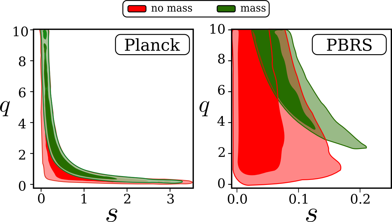
In Sec. III.2 we discussed how the parameter space changes when including the mass condition as prior on top of the baseline stability conditions. In this section we discuss the impact of such condition on the cosmological and model parameters when . We notice that such condition does not affect the constraints on the cosmological parameters, while it has an effect only on the model parameters. We show in Figure 10, the confidence regions for and obtained using the Planck CMB temperature and polarization data when only the baseline stability conditions are imposed (red) and the case in which the mass condition is included (green). As expected the constraints follow the shape of the stability cut induced by the mass condition. As previously discussed, the parameter space of and does not change when considering higher values of (), thus the green contours in Figure 10 hold also for such values of . From our analysis we note that alone does not add much information to the stability condition , while the inclusion of BAO data in the complete dataset push the lower bound to an higher value, for the model without massive neutrinos and with massive neutrinos. The higher lower bound on obtained with the extended data sets is motivated by the fact that BAO+RSD+SNIa data (in particular BAO) strongly constrain the parameters at background level. For this case we obtain with alone, while give the tighter constraint . The marginalized constraint on with massive neutrinos does not change for the data, while its central value with data alone is smaller . Thus BAO data push the values of toward zero and as consequences they select higher values of . The latter is a consequence of the mass condition according to which small value of select higher values of .

| Model | (eV) | |||||
|---|---|---|---|---|---|---|
| CDM () | - | - | - | |||
| CDM () | - | - | - | |||
| CDM+ () | - | - | ||||
| CDM+ () | - | - | ||||
| GCCG () | - | |||||
| GCCG () | - | |||||
| GCCG + () | ||||||
| GCCG + () |
V Conclusion
In this work we have performed a thorough investigation of the impact on the cosmological observables of the modification induced by a specific class of Galileon models, the generalized cubic covariant Galileon (GCCG). Compared to CDM the model introduces two extra parameters of which only affects the background dynamics, while both introduce modifications at linear perturbation level. We have identified modifications in the ISW effect, the gravitational lensing, the rate of growth of structure and temperature-temperature power spectrum at large angular scales. While both the lensing and the matter power spectra are in general enhanced with respect to CDM, the low- TT power spectrum can be either enhanced or suppressed and the high- peaks are shifted due to a modified background evolution. We found that the inclusion of massive neutrinos generally brings down the deviations of GCCG from CDM. We have performed cosmological constraints considering data from CMB, BAO, RSD, SNIa and Cepheids () in different combinations in order to identify how different data sets contribute to the parameter bounds. The results are shown in Tab. 3. Notably, we found that GCCG is able to ease the tension in the estimation of the present day value of the Hubble parameter between Planck and low- measurements which arises within CDM. However the tension is again present when we include BAO data. This case needs a further investigation as BAO data might be biased toward CDM-like models Carter et al. 2019. We found that the tightest constraints for at 95% C.L are for the data set, while shows only a lower bound . The joint analysis with Planck and instead is able to set the upper bound . We also found a lower bound for the sum of the neutrino masses to be eV at along with the usual upper bound. This is an interesting result which should be further considered in light of future results from experiments measuring the neutrino mass.
The model selection analysis shows that the extended model is favored over CDM when considering the Planck data alone, because the GCCG is able to better fit the ISW tail. Nevertheless, the complete dataset points toward the standard cosmological model with a DIC value that indicates a mild preference for the latter. These results suggest that further work is needed in order to asses the statistical preference of one cosmological model over the other and it will be the subject of upcoming projects.
This study is a further proof that Galileon models cannot be definitely excluded with respect to CDM . Indeed besides the model investigated here there is another case in which the data support the Galileon cosmology over CDM , the Galileon ghost condensate model Peirone et al. 2019. In this regard it will be essential to test Galileon models with next generation surveys, which will offer us the possibility to test gravity at cosmological scales with unprecedented accuracy.
Acknowledgements.
We thank M. Raveri, A. Silvestri, M. Vicinanza, and L. Yin for useful discussions. NF and LA are supported by Fundação para a Ciência e a Tecnologia (FCT) through national funds (UID/FIS/04434/2019), by FEDER through COMPETE2020 (POCI-01-0145-FEDER-007672). The research of NF is also supported by FCT project “DarkRipple – Spacetime ripples in the dark gravitational Universe” with ref. number PTDC/FIS-OUT/29048/2017. SP acknowledges support from the NWO and the Dutch Ministry of Education, Culture and Science (OCW), and also from the D-ITP consortium, a program of the NWO that is funded by the OCW. NF and SP acknowledge the COST Action (CANTATA/CA15117), supported by COST (European Cooperation in Science and Technology).References
- Joyce et al. (2015) A. Joyce, B. Jain, J. Khoury, and M. Trodden, Phys. Rept. 568, 1 (2015), arXiv:1407.0059 [astro-ph.CO] .
- Lue et al. (2004) A. Lue, R. Scoccimarro, and G. D. Starkman, Phys. Rev. D69, 124015 (2004), arXiv:astro-ph/0401515 [astro-ph] .
- Copeland et al. (2006) E. J. Copeland, M. Sami, and S. Tsujikawa, Int. J. Mod. Phys. D15, 1753 (2006), arXiv:hep-th/0603057 [hep-th] .
- Silvestri and Trodden (2009) A. Silvestri and M. Trodden, Rept. Prog. Phys. 72, 096901 (2009), arXiv:0904.0024 [astro-ph.CO] .
- Capozziello and De Laurentis (2011) S. Capozziello and M. De Laurentis, Phys. Rept. 509, 167 (2011), arXiv:1108.6266 [gr-qc] .
- Clifton et al. (2012) T. Clifton, P. G. Ferreira, A. Padilla, and C. Skordis, Phys. Rept. 513, 1 (2012), arXiv:1106.2476 [astro-ph.CO] .
- Tsujikawa (2010) S. Tsujikawa, Lect. Notes Phys. 800, 99 (2010), arXiv:1101.0191 [gr-qc] .
- Koyama (2016) K. Koyama, Rept. Prog. Phys. 79, 046902 (2016), arXiv:1504.04623 [astro-ph.CO] .
- Ferreira (2019) P. G. Ferreira, (2019), 10.1146/annurev-astro-091918-104423, arXiv:1902.10503 [astro-ph.CO] .
- Kobayashi (2019) T. Kobayashi, Rept. Prog. Phys. 82, 086901 (2019), arXiv:1901.07183 [gr-qc] .
- Horndeski (1974) G. W. Horndeski, Int. J. Theor. Phys. 10, 363 (1974).
- Deffayet et al. (2009a) C. Deffayet, S. Deser, and G. Esposito-Farese, Phys. Rev. D80, 064015 (2009a), arXiv:0906.1967 [gr-qc] .
- Kase and Tsujikawa (2018) R. Kase and S. Tsujikawa, Phys. Rev. D97, 103501 (2018), arXiv:1802.02728 [gr-qc] .
- Peirone et al. (2019) S. Peirone, G. Benevento, N. Frusciante, and S. Tsujikawa, Phys. Rev. D100, 063540 (2019), arXiv:1905.05166 [astro-ph.CO] .
- De Felice and Tsujikawa (2012a) A. De Felice and S. Tsujikawa, JCAP 1202, 007 (2012a), arXiv:1110.3878 [gr-qc] .
- Deffayet et al. (2009b) C. Deffayet, G. Esposito-Farese, and A. Vikman, Phys. Rev. D79, 084003 (2009b), arXiv:0901.1314 [hep-th] .
- De Felice and Tsujikawa (2010) A. De Felice and S. Tsujikawa, Phys. Rev. Lett. 105, 111301 (2010), arXiv:1007.2700 [astro-ph.CO] .
- De Felice and Tsujikawa (2011) A. De Felice and S. Tsujikawa, Phys. Rev. D84, 124029 (2011), arXiv:1008.4236 [hep-th] .
- Frusciante et al. (2019a) N. Frusciante, R. Kase, K. Koyama, S. Tsujikawa, and D. Vernieri, Phys. Lett. B790, 167 (2019a), arXiv:1812.05204 [gr-qc] .
- De Felice and Tsujikawa (2012b) A. De Felice and S. Tsujikawa, JCAP 1203, 025 (2012b), arXiv:1112.1774 [astro-ph.CO] .
- Renk et al. (2017) J. Renk, M. Zumalacarregui, F. Montanari, and A. Barreira, JCAP 1710, 020 (2017), arXiv:1707.02263 [astro-ph.CO] .
- Peirone et al. (2018) S. Peirone, N. Frusciante, B. Hu, M. Raveri, and A. Silvestri, Phys. Rev. D97, 063518 (2018), arXiv:1711.04760 [astro-ph.CO] .
- Leloup et al. (2019) C. Leloup, V. Ruhlmann-Kleider, J. Neveu, and A. De Mattia, JCAP 1905, 011 (2019), arXiv:1902.07065 [astro-ph.CO] .
- Abbott et al. (2017a) B. Abbott et al. (Virgo, LIGO Scientific), Phys. Rev. Lett. 119, 161101 (2017a), arXiv:1710.05832 [gr-qc] .
- Coulter et al. (2017) D. A. Coulter et al., Science (2017), 10.1126/science.aap9811, arXiv:1710.05452 [astro-ph.HE] .
- Abbott et al. (2017b) B. P. Abbott et al., Astrophys. J. 848, L12 (2017b), arXiv:1710.05833 [astro-ph.HE] .
- Creminelli and Vernizzi (2017) P. Creminelli and F. Vernizzi, Phys. Rev. Lett. 119, 251302 (2017), arXiv:1710.05877 [astro-ph.CO] .
- Ezquiaga and Zumalacsrregui (2017) J. M. Ezquiaga and M. Zumalacsrregui, Phys. Rev. Lett. 119, 251304 (2017), arXiv:1710.05901 [astro-ph.CO] .
- Baker et al. (2017) T. Baker, E. Bellini, P. G. Ferreira, M. Lagos, J. Noller, and I. Sawicki, Phys. Rev. Lett. 119, 251301 (2017), arXiv:1710.06394 [astro-ph.CO] .
- Sakstein and Jain (2017) J. Sakstein and B. Jain, Phys. Rev. Lett. 119, 251303 (2017), arXiv:1710.05893 [astro-ph.CO] .
- Bettoni et al. (2017) D. Bettoni, J. M. Ezquiaga, K. Hinterbichler, and M. Zumalacárregui, Phys. Rev. D95, 084029 (2017), arXiv:1608.01982 [gr-qc] .
- Kase and Tsujikawa (2019) R. Kase and S. Tsujikawa, Int. J. Mod. Phys. D28, 1942005 (2019), arXiv:1809.08735 [gr-qc] .
- Giacomello et al. (2019) F. Giacomello, A. De Felice, and S. Ansoldi, JCAP 1903, 038 (2019), arXiv:1811.10885 [astro-ph.CO] .
- Barreira et al. (2014) A. Barreira, B. Li, C. Baugh, and S. Pascoli, JCAP 1408, 059 (2014), arXiv:1406.0485 [astro-ph.CO] .
- Kobayashi et al. (2010a) T. Kobayashi, H. Tashiro, and D. Suzuki, Phys. Rev. D81, 063513 (2010a), arXiv:0912.4641 [astro-ph.CO] .
- Gubitosi et al. (2013) G. Gubitosi, F. Piazza, and F. Vernizzi, JCAP 1302, 032 (2013), [JCAP1302,032(2013)], arXiv:1210.0201 [hep-th] .
- Bloomfield et al. (2013) J. K. Bloomfield, E. E. Flanagan, M. Park, and S. Watson, JCAP 1308, 010 (2013), arXiv:1211.7054 [astro-ph.CO] .
- Hu et al. (2014a) B. Hu, M. Raveri, N. Frusciante, and A. Silvestri, Phys. Rev. D89, 103530 (2014a), arXiv:1312.5742 [astro-ph.CO] .
- Raveri et al. (2014) M. Raveri, B. Hu, N. Frusciante, and A. Silvestri, Phys. Rev. D90, 043513 (2014), arXiv:1405.1022 [astro-ph.CO] .
- Lesgourgues and Pastor (2006) J. Lesgourgues and S. Pastor, Phys. Rept. 429, 307 (2006), arXiv:astro-ph/0603494 [astro-ph] .
- Wong (2011) Y. Y. Y. Wong, Ann. Rev. Nucl. Part. Sci. 61, 69 (2011), arXiv:1111.1436 [astro-ph.CO] .
- Riess et al. (2011) A. G. Riess, L. Macri, S. Casertano, H. Lampeitl, H. C. Ferguson, A. V. Filippenko, S. W. Jha, W. Li, and R. Chornock, Astrophys. J. 730, 119 (2011), [Erratum: Astrophys. J.732,129(2011)], arXiv:1103.2976 [astro-ph.CO] .
- Riess et al. (2016) A. G. Riess et al., Astrophys. J. 826, 56 (2016), arXiv:1604.01424 [astro-ph.CO] .
- Riess et al. (2019) A. G. Riess, S. Casertano, W. Yuan, L. M. Macri, and D. Scolnic, Astrophys. J. 876, 85 (2019), arXiv:1903.07603 [astro-ph.CO] .
- Delubac et al. (2015) T. Delubac et al. (BOSS), Astron. Astrophys. 574, A59 (2015), arXiv:1404.1801 [astro-ph.CO] .
- Abbott et al. (2018a) T. M. C. Abbott et al. (DES), Phys. Rev. D98, 043526 (2018a), arXiv:1708.01530 [astro-ph.CO] .
- Abbott et al. (2018b) T. M. C. Abbott et al. (DES), Mon. Not. Roy. Astron. Soc. 480, 3879 (2018b), arXiv:1711.00403 [astro-ph.CO] .
- Freedman et al. (2019) W. L. Freedman et al., (2019), 10.3847/1538-4357/ab2f73, arXiv:1907.05922 [astro-ph.CO] .
- Yuan et al. (2019) W. Yuan, A. G. Riess, L. M. Macri, S. Casertano, and D. Scolnic, Astrophys. J. 886, 61 (2019), arXiv:1908.00993 [astro-ph.GA] .
- Karwal and Kamionkowski (2016) T. Karwal and M. Kamionkowski, Phys. Rev. D94, 103523 (2016), arXiv:1608.01309 [astro-ph.CO] .
- Pourtsidou and Tram (2016) A. Pourtsidou and T. Tram, Phys. Rev. D94, 043518 (2016), arXiv:1604.04222 [astro-ph.CO] .
- Poulin et al. (2019) V. Poulin, T. L. Smith, T. Karwal, and M. Kamionkowski, Phys. Rev. Lett. 122, 221301 (2019), arXiv:1811.04083 [astro-ph.CO] .
- Lin et al. (2019) M.-X. Lin, M. Raveri, and W. Hu, Phys. Rev. D99, 043514 (2019), arXiv:1810.02333 [astro-ph.CO] .
- Agrawal et al. (2019a) P. Agrawal, G. Obied, and C. Vafa, (2019a), arXiv:1906.08261 [astro-ph.CO] .
- Agrawal et al. (2019b) P. Agrawal, F.-Y. Cyr-Racine, D. Pinner, and L. Randall, (2019b), arXiv:1904.01016 [astro-ph.CO] .
- Kaloper (2019) N. Kaloper, Int. J. Phys. D (2019), 10.1142/S0218271819440176, arXiv:1903.11676 [hep-th] .
- Desmond et al. (2019) H. Desmond, B. Jain, and J. Sakstein, Phys. Rev. D100, 043537 (2019), arXiv:1907.03778 [astro-ph.CO] .
- Di Valentino et al. (2019) E. Di Valentino, A. Melchiorri, O. Mena, and S. Vagnozzi, (2019), arXiv:1910.09853 [astro-ph.CO] .
- Sakstein and Trodden (2019) J. Sakstein and M. Trodden, (2019), arXiv:1911.11760 [astro-ph.CO] .
- Lombriser (2019) L. Lombriser, (2019), arXiv:1906.12347 [astro-ph.CO] .
- Deffayet et al. (2010) C. Deffayet, O. Pujolas, I. Sawicki, and A. Vikman, JCAP 1010, 026 (2010), arXiv:1008.0048 [hep-th] .
- Kobayashi et al. (2010b) T. Kobayashi, M. Yamaguchi, and J. Yokoyama, Phys. Rev. Lett. 105, 231302 (2010b), arXiv:1008.0603 [hep-th] .
- Barreira et al. (2013) A. Barreira, B. Li, C. M. Baugh, and S. Pascoli, JCAP 1311, 056 (2013), arXiv:1308.3699 [astro-ph.CO] .
- Barreira et al. (2014) A. Barreira, B. Li, C. M. Baugh, and S. Pascoli, jcap 8, 059 (2014), arXiv:1406.0485 .
- Gleyzes et al. (2013) J. Gleyzes, D. Langlois, F. Piazza, and F. Vernizzi, JCAP 1308, 025 (2013), arXiv:1304.4840 [hep-th] .
- Piazza et al. (2014) F. Piazza, H. Steigerwald, and C. Marinoni, JCAP 1405, 043 (2014), arXiv:1312.6111 [astro-ph.CO] .
- Tsujikawa (2015) S. Tsujikawa, Lect. Notes Phys. 892, 97 (2015), arXiv:1404.2684 [gr-qc] .
- Frusciante and Perenon (2019) N. Frusciante and L. Perenon, (2019), arXiv:1907.03150 [astro-ph.CO] .
- Hu et al. (2014b) B. Hu, M. Raveri, N. Frusciante, and A. Silvestri, (2014b), arXiv:1405.3590 [astro-ph.IM] .
- Bloomfield (2013) J. Bloomfield, JCAP 1312, 044 (2013), arXiv:1304.6712 [astro-ph.CO] .
- Gleyzes et al. (2015a) J. Gleyzes, D. Langlois, and F. Vernizzi, Int. J. Mod. Phys. D23, 1443010 (2015a), arXiv:1411.3712 [hep-th] .
- Frusciante et al. (2016a) N. Frusciante, M. Raveri, D. Vernieri, B. Hu, and A. Silvestri, Phys. Dark Univ. 13, 7 (2016a), arXiv:1508.01787 [astro-ph.CO] .
- Frusciante et al. (2016b) N. Frusciante, G. Papadomanolakis, and A. Silvestri, JCAP 1607, 018 (2016b), arXiv:1601.04064 [gr-qc] .
- Frusciante et al. (2019b) N. Frusciante, S. Peirone, S. Casas, and N. A. Lima, Phys. Rev. D99, 063538 (2019b), arXiv:1810.10521 [astro-ph.CO] .
- Gleyzes et al. (2015b) J. Gleyzes, D. Langlois, F. Piazza, and F. Vernizzi, JCAP 1502, 018 (2015b), arXiv:1408.1952 [astro-ph.CO] .
- Gergely and Tsujikawa (2014) L. A. Gergely and S. Tsujikawa, Phys. Rev. D89, 064059 (2014), arXiv:1402.0553 [hep-th] .
- Kase and Tsujikawa (2014) R. Kase and S. Tsujikawa, Phys. Rev. D90, 044073 (2014), arXiv:1407.0794 [hep-th] .
- De Felice et al. (2015) A. De Felice, K. Koyama, and S. Tsujikawa, JCAP 1505, 058 (2015), arXiv:1503.06539 [gr-qc] .
- De Felice et al. (2017) A. De Felice, N. Frusciante, and G. Papadomanolakis, JCAP 1703, 027 (2017), arXiv:1609.03599 [gr-qc] .
- Frusciante et al. (2019c) N. Frusciante, G. Papadomanolakis, S. Peirone, and A. Silvestri, JCAP 1902, 029 (2019c), arXiv:1810.03461 [gr-qc] .
- Bean and Tangmatitham (2010) R. Bean and M. Tangmatitham, Phys. Rev. D81, 083534 (2010), arXiv:1002.4197 [astro-ph.CO] .
- Silvestri et al. (2013) A. Silvestri, L. Pogosian, and R. V. Buniy, Phys. Rev. D87, 104015 (2013), arXiv:1302.1193 [astro-ph.CO] .
- Aghanim et al. (2016) N. Aghanim et al. (Planck), Astron. Astrophys. 594, A11 (2016), arXiv:1507.02704 [astro-ph.CO] .
- Ade et al. (2016) P. A. R. Ade et al. (Planck), Astron. Astrophys. 594, A13 (2016), arXiv:1502.01589 [astro-ph.CO] .
- Aghanim et al. (2018) N. Aghanim et al. (Planck), (2018), arXiv:1807.06209 [astro-ph.CO] .
- Beutler et al. (2011) F. Beutler, C. Blake, M. Colless, D. H. Jones, L. Staveley-Smith, L. Campbell, Q. Parker, W. Saunders, and F. Watson, mnras 416, 3017 (2011), arXiv:1106.3366 .
- Ross et al. (2015) A. J. Ross, L. Samushia, C. Howlett, W. J. Percival, A. Burden, and M. Manera, mnras 449, 835 (2015), arXiv:1409.3242 .
- Alam et al. (2017) S. Alam et al. (BOSS), Mon. Not. Roy. Astron. Soc. 470, 2617 (2017), arXiv:1607.03155 [astro-ph.CO] .
- Betoule et al. (2014) M. Betoule et al. (SDSS), Astron. Astrophys. 568, A22 (2014), arXiv:1401.4064 [astro-ph.CO] .
- Asgari et al. (2019) M. Asgari et al., (2019), arXiv:1910.05336 [astro-ph.CO] .
- de Jong et al. (2015) J. T. A. de Jong et al., Astron. Astrophys. 582, A62 (2015), arXiv:1507.00742 [astro-ph.CO] .
- Carter et al. (2019) P. Carter, F. Beutler, W. J. Percival, J. DeRose, R. H. Wechsler, and C. Zhao, (2019), arXiv:1906.03035 [astro-ph.CO] .
- Aker et al. (2019) M. Aker et al. (KATRIN), Phys. Rev. Lett. 123, 221802 (2019), arXiv:1909.06048 [hep-ex] .
- Crittenden and Turok (1996) R. G. Crittenden and N. Turok, Phys. Rev. Lett. 76, 575 (1996), arXiv:astro-ph/9510072 [astro-ph] .
- Boughn et al. (1998) S. P. Boughn, R. G. Crittenden, and N. G. Turok, New Astron. 3, 275 (1998), arXiv:astro-ph/9704043 [astro-ph] .
- Kimura et al. (2012) R. Kimura, T. Kobayashi, and K. Yamamoto, Phys. Rev. D85, 123503 (2012), arXiv:1110.3598 [astro-ph.CO] .
- Spiegelhalter et al. (2014) D. J. Spiegelhalter, N. G. Best, B. P. Carlin, and A. van der Linde, Journal of the Royal Statistical Society: Series B (Statistical Methodology) 76, 485 (2014).
- Creminelli et al. (2019) P. Creminelli, G. Tambalo, F. Vernizzi, and V. Yingcharoenrat, (2019), arXiv:1910.14035 [gr-qc] .
- de Rham and Melville (2018) C. de Rham and S. Melville, Phys. Rev. Lett. 121, 221101 (2018), arXiv:1806.09417 [hep-th] .