FIRST ANALYTICAL CALCULATION
OF BLACK HOLE SHADOW IN MCVITTIE METRIC

To apply the method, we need to have two asymptotic analytical solutions, usually called ’inner’ and ’outer’. We also need to have an overlap region where both of these solutions should be valid. The existence of this region allows to match two solutions, finding unknown constants. Moreover, the method allows to write an approximate solution (usually called ’composite’) that will be valid for the entire range of variable [84, 85].

McVittie metric has a form

$a(t)$ is the scale factor, $m=GM/c^{2}$ is mass parameter, with $M$ being the black hole mass. In asymptotic cases the McVittie metric is reduced to the Schwarzschild metric and to the Friedmann-Robertson-Walker (FRW) metric (see below).

We are interested in finding out what size of the shadow is observed by a comoving observer located at $\rho_{O}$ at the time $t_{O}$. As mentioned above, an exact analytic solution for angular size of BH shadow valid for arbitrary observer’s position is not found yet. Our goal is to find an approximate solution using the method described above. For that, we will match two asymptotic solutions, known for Schwarzschild and FRW cases, $\alpha_{schw}$ and $\alpha_{cosm}$.

With $a(t)\equiv\mbox{const}$, the McVittie metric (1) is simplified to the Schwarzschild metric in isotropic coordinates. Since we are interested in a non-trivial case $a(t)\not\equiv\mbox{const}$, we need to understand at what scales we can consider the scale factor as constant. Physically, expansion is negligible if the observer is close to a black hole, and redshift is small: $z\ll 1$. Indeed, we can write the scale factor $a(t)$ as [93]

If $t_{0}-t\ll H_{0}^{-1}$, we may write that $a(t)\simeq a(t_{0})$. For small values of $(t_{0}-t)$ we can write $z\simeq(t_{0}-t)H_{0}$ [93], so we obtain finally:

With $a(t)=a(t_{0})$ the metric (1) is reduced to the form where all coefficients are independent on time:

With the help of new variable

time-independent metric (5) can be reduced to the Schwarzschild metric in isotropic coordinates:

Further, introducing the variable

the usual form of Schwarzschild metric is recovered:

Note that $R=r$ if $m\to 0$.

Let us consider the comoving observer in the spacetime (5). An observer has a radial coordinate $\rho_{O}$ and observes the shadow at a time $t_{O}$. Obviously, the time of observation $t_{O}$ coincides with the present time $t_{0}$ introduced earlier. We denote the observer’s position in new variables as

For the Schwarzschild metric in the form (10), the angular size of the shadow is given by [7] as

Noting that $0<\alpha_{schw}\leq\pi/2$ for $R_{O}\geq 3m$, and $\pi/2\leq\alpha_{schw}\leq\pi$ for $2m\leq R_{O}\leq 3m$, we write the angle as

For $m/\rho\to 0$, that is at large distances from BH, the McVittie metric (1) is simplified to FRW metric written in comoving coordinates:

Apparent angular size $\alpha$ of any object of known physical size $L$ as seen by comoving observer in expanding FRW universe can be calculated as [89, 90, 91, 92, 93, 94]

where $D_{A}(z)$ is the angular diameter distance. In the flat $\Lambda$CDM model it can be written as [93, 95]

where

Here $H_{0}$ is the present value of the Hubble parameter $H(t_{0})$, and $\Omega_{m0}$, $\Omega_{r0}$, $\Omega_{\Lambda 0}$ are the present dimensionless density parameters for matter, radiation and dark energy, respectively.

Since for $r\gg m$ the McVittie metric tends to FRW metric, we can use the formula (15) for calculation of angular size of the shadow for comoving observer at large distances:

The only crucial difference from FRW case without BH is that we don’t know the value of $L_{\mathrm{sh}}$ which is now the effective linear radius of the shadow. Specific value $L_{\mathrm{sh}}$ is determined by strong bending of light rays in the vicinity of BH. We will find this unknown constant later, by matching two solutions. Note that formula (18) implies that the angle $\alpha_{cosm}$ is small.

Eq.(18) is written as a function of $z$, but we need to have it as a function of radial coordinate. For transformation, the following formula can be used [93, 95]:

where $H(\tilde{z})$ is defined in eq.(17). Further, it is more convenient to use $R_{O}$ instead of $r_{O}$. At large distances from the black hole, $r\gg m$, the variables of $r$ and $R$ coincide. Therefore we can write the connection between $R_{O}$ and $z$:

Substitution of $z$ expressed via $R_{O}$ into (18) gives the $\alpha_{cosm}$ as a function of $R_{O}$.

Now we have two solutions, $\alpha_{schw}(R_{O})$ and $\alpha_{cosm}(R_{O})$, which we would like to match.

Idea of matching is based on existence of overlap region where both solutions should be valid. To connect the expansions, we introduce an intermediate variable which is to be located within the overlap region [84]. Intermediate variable $R_{int}$ should satisfy the condition:

where $R_{inner}$ and $R_{outer}$ are characteristic scales of inner and outer solutions validity. To match the expansions, the inner and outer approximations must give the same result when the intermediate value is substituted.

In our problem, the overlap region is an almost flat space-time between the black hole and the region of rapid expansion. On the one hand, this region is far enough from the black hole so that its gravity can be considered as negligible. On the other hand, the scales are still small enough so that cosmic expansion can be neglected.

First condition is $R\gg m$. Second condition can be obtained from the condition $z\ll 1$. With using of relation (20) for small $z$, this leads to $R\ll c/H_{0}$. Finally, we obtain the condition for overlap region and intermediate variable as

To conclude: for given $m$ and $H_{0}$, the matching is possible only if it is possible to introduce the value $R_{int}$ which satisfy the condition (22). Similar condition was used in our previous paper to find the solution at large cosmological distances [62].

For $R_{O}\gg m$, the solution (13) is simplified to

At the same time, for $R_{O}\ll c/H_{0}$ ($z\ll 1$), the angular diameter distance $D_{A}(z)$ is simplified to $r_{O}$ (which coincides with $R_{O}$ for $r\gg m$ ), and we obtain from eq. (18) that

Considering $R_{O}$ from the intermediate region (22) we match two solutions (23) and (24) at this point, which gives the value of constant $L_{\mathrm{sh}}$:

Substituting $L_{\mathrm{sh}}$ into formula (18), we find that the outer asymptotic solution equals to:

Solution (26) was constructed in our previous paper [62] by using physical reasons.

A composite solution is an approximation valid for arbitrary value of the variable $R_{O}$. It is constructed as [84]

Here the overlap value is equal to the inner solution (23) or to the outer solution (24) in the intermediate region. So, for $R_{O}$ inside the intermediate region $R_{int}$ we obtain

Finally, we have the resulting composite solution defined by Eq.(27) where $\alpha_{schw}(R_{O})$ is defined in (13), $\alpha_{cosm}(R_{O})$ is defined in (26), and $z$ is expressed through $R_{O}$ by formula (20).

We start from the black hole embedded into de Sitter universe. This can be described by Kottler (Schwarzschild-de-Sitter) solution, which is a particular case of the McVittie metric. For this case we have:

The formula (26) gives that

The formula (20) gives

After substitution of (31) into (30), we obtain finally the approximate solution in the form:

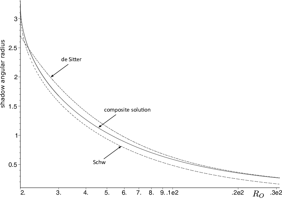
Note that, due to condition (22), the second term is small ($\ll 1$). The approximate solution is shown in Fig.  1.

For the particular case of Kottler metric, the exact solution for angular size of the shadow is known. The shadow angular radius as seen by the comoving observer is defined by the expression [61]

Here the minus sign should be chosen for $R_{H1}<R_{O}<3m$, and the plus sign for $3m<R_{O}<\infty$ ($R_{H1}$ is black hole event horizon size in Kottler metric). Using the formula for the sine of the sum,

and properties of trigonometrical functions, we can rewrite (33) in the simple form:

where $\alpha_{schw}$ is defined by Synge’s formula, see (12) and (13).

The approximate solution (32) coincides with the exact one (35) because at small argument of arcsin we have $\arcsin x\approx x$.

Let us consider the case of a black hole in the flat dusty Friedmann universe model (also known as Einstein-de-Sitter model) [93, 94]. This model has the following cosmological parameters: $\Omega_{m0}=1$, $\Omega_{r0}=0$, $\Omega_{\Lambda 0}=0$, $a(t)=(3H_{0}t/2)^{2/3}$. For $\alpha_{cosm}$ we have:

The formula (20) gives

Finally, we obtain for $\alpha_{cosm}(R_{O})$:

Using (38) in (27) gives the approximate solution for $\alpha_{appr}$, which is plotted in Fig. 2.

References

- [1] K. Akiyama et al (Event Horizon Telescope Collaboration), The Astrophysical Journal Letters 875 (2019) L1.
- [2] K. Akiyama et al (Event Horizon Telescope Collaboration), The Astrophysical Journal Letters 875 (2019) L2.
- [3] K. Akiyama et al (Event Horizon Telescope Collaboration), The Astrophysical Journal Letters 875 (2019) L3.
- [4] K. Akiyama et al (Event Horizon Telescope Collaboration), The Astrophysical Journal Letters 875 (2019) L4.
- [5] K. Akiyama et al (Event Horizon Telescope Collaboration), The Astrophysical Journal Letters 875 (2019) L5.
- [6] K. Akiyama et al (Event Horizon Telescope Collaboration), The Astrophysical Journal Letters 875 (2019) L6.
- [7] J. L. Synge, Mon. Not. R. Astron. Soc. 131 (1966) 463.
- [8] J. M. Bardeen, Timelike and null geodesics in the Kerr metric, in Black Holes, edited by C. DeWitt and B. DeWitt (Gordon and Breach, New York, 1973), p. 215.
- [9] J.-P. Luminet, Astron. Astrophys. 75 (1979) 228.
- [10] S. Chandrasekhar, The Mathematical Theory of Black Holes (Clarendon Press, Oxford, 1983).
- [11] I. G. Dymnikova, Sov. Phys. Usp. 29 (1986) 215.
- [12] H. Falcke, F. Melia, and E. Agol, Astrophys. Journal Lett. 528 (2000) L13.
- [13] R. Takahashi, The Astrophysical Journal 611 (2004) 996.
- [14] K. Hioki and K. Maeda, Phys. Rev. D 80 (2009) 024042.
- [15] M. Mościbrodzka, C.F. Gammie, J.C. Dolence, et al., The Astrophysical Journal 706 (2009) 497.
- [16] T. Johannsen and D. Psaltis, The Astrophysical Journal 718 (2010) 446.
- [17] V.P. Frolov and A. Zelnikov, Introduction to Black Hole Physics (Oxford University Press, Oxford, 2011).
- [18] C. Bambi and L. Modesto, Phys. Lett. B 721 (2013) 329.
- [19] A. Grenzebach, V. Perlick, and C. Lämmerzahl, Phys. Rev. D 89 (2014) 124004.
- [20] R.-S. Lu, A. E. Broderick, F. Baron, et al., The Astrophysical Journal 788 (2014) 120.
- [21] N. Tsukamoto, Z. Li and C. Bambi, J. Cosmol. Astropart. Phys. 06 (2014) 043.
- [22] A.F. Zakharov, Phys. Rev. D 90 (2014) 062007.
- [23] A. Grenzebach, V. Perlick, and C. Lämmerzahl, Int. J. Mod. Phys. D 24 (2015) 1542024.
- [24] O. James, E. Tunzelmann, P. Franklin, and K. Thorne, Class. Quantum Grav. 32 (2015) 065001.
- [25] P. V. P. Cunha, C. A. R. Herdeiro, E. Radu, and H. F. Rúnarsson, Phys. Rev. Lett. 115 (2015) 211102.
- [26] V. Perlick, O. Yu. Tsupko, and G. S. Bisnovatyi-Kogan, Phys. Rev. D 92 (2015) 104031.
- [27] A. A. Abdujabbarov, L. Rezzolla, and B. J. Ahmedov, Mon. Not. R. Astron. Soc. 454 (2015) 2423.
- [28] T. Johannsen, A. E. Broderick, P. M. Plewa, et al., Phys. Rev. Lett. 116 (2016) 031101.
- [29] R. Konoplya, L. Rezzolla and A. Zhidenko, Phys. Rev. D 93 (2016) 064015.
- [30] J. O. Shipley and S. R. Dolan, Class and Quant Grav 33 (2016) 175001
- [31] S.S. Doeleman, Nature Astronomy 1 (2017) 646.
- [32] V. Perlick and O. Yu. Tsupko, Phys. Rev. D 95 (2017) 104003.
- [33] O. Yu. Tsupko, Phys. Rev. D 95 (2017) 104058.
- [34] C. Goddi, H. Falcke, M. Kramer, et al, International Journal of Modern Physics D 26 (2017) 1730001-239.
- [35] P. V. P. Cunha, C. A. R. Herdeiro, B. Kleihaus, J. Kunz, and E. Radu, Phys. Lett. B 768 (2017) 373.
- [36] E. F. Eiroa and C. M. Sendra, The European Physical Journal C 78 (2018) 91.
- [37] N. Tsukamoto, Phys. Rev. D 97 (2018) 064021.
- [38] P. V. P. Cunha and C. A. R. Herdeiro, General Relativity and Gravitation 50 (2018) 42.
- [39] Y. Mizuno, Z. Younsi, C.M. Fromm, et al., Nature Astronomy 2 (2018) 585.
- [40] M. Mars, C.F. Paganini and M.A. Oancea, Class and Quant Grav 35 (2018) 025005
- [41] D. Ayzenberg and N. Yunes, Class and Quant Grav 35 (2018) 235002.
- [42] R. Kumar and S.G. Ghosh, eprint arXiv:1811.01260 (2018).
- [43] G. Gyulchev, P. Nedkova, V. Tinchev, S. Yazadjiev, The European Physical Journal C 78 (2018) 544.
- [44] B.P. Singh and S.G. Ghosh, Annals of Physics 395 (2018) 127
- [45] H. Gott, D. Ayzenberg, N. Yunes and A. Lohfink, Class and Quant Grav 36 (2019) 055007
- [46] V. I. Dokuchaev, N. O. Nazarova and V. P. Smirnov, General Relativity and Gravitation 51 (2019) 81
- [47] S. E. Gralla, D. E. Holz and R. M. Wald, Phys. Rev. D 100 (2019) 024018
- [48] M.D. Johnson, A. Lupsasca, A. Strominger, et al, eprint arXiv: 1907.04329 (2019)
- [49] R. Narayan, M.D. Johnson, C.F. Gammie, ApJL 885 (2019) L33
- [50] R. A. Konoplya, Physics Letters B 795 (2019) 1.
- [51] V.I. Dokuchaev, N.O. Nazarova, eprint arXiv: 1911.07695 (2019)
- [52] K. Jusufi, eprint arXiv:1912.13320 (2019)
- [53] R. Shaikh, Physical Review D 100 (2019) 024028.
- [54] Takahisa Igata, Hideki Ishihara, and Yu Yasunishi, Phys. Rev. D 100 (2019) 044058.
- [55] S. O. Alexeyev, B. N. Latosh, V. A. Prokopov and E. D. Emtsova, Journal of Experimental and Theoretical Physics, 128 (2019) 720.
- [56] Shao-Wen Wei, Yuan-Chuan Zou, Yu-Xiao Liu and Robert B. Mann, Journal of Cosmology and Astroparticle Physics 08 (2019) 030.
- [57] F. Kottler, Ann. Phys. (Berlin) 361 (1918) 401.
- [58] Z. Stuchlík and S. Hledík, Physical Review D 60 (1999) 044006.
- [59] P. Bakala, P. Čermák, S. Hledík, Z. Stuchlík, and K. Truparová, Central European Journal of Physics 5 (2007) 599.
- [60] Z. Stuchlík, D. Charbulák, and J. Schee, Eur. Phys. J. C 78 (2018) 180.
- [61] V. Perlick, O. Yu. Tsupko, and G. S. Bisnovatyi-Kogan, Physical Review D 97 (2018) 104062.
- [62] G. S. Bisnovatyi-Kogan and O. Yu. Tsupko, Physical Review D 98 (2018) 084020.
- [63] O.Yu. Tsupko, Z. Fan, and G.S. Bisnovatyi-Kogan, Classical and Quantum Gravity 37 (2020) 065016; arXiv:1905.10509
- [64] Jing-Zhao Qi and Xin Zhang, eprint arXiv: 1906.10825 (2019)
- [65] S. Vagnozzi, C. Bambi, and L. Visinelli, eprint arXiv: 2001.02986 (2020)
- [66] G. C. McVittie, Mon. Not. Roy. Astron. Soc. 93 (1933) 325.
- [67] B. C. Nolan, Phys. Rev. D 58 (1998) 064006.
- [68] B. C. Nolan, Class. Quantum Grav. 16 (1999a) 1227.
- [69] B. C. Nolan, Class. Quantum Grav. 16 (1999b) 3183.
- [70] N. Kaloper, M. Kleban, and D. Martin, Phys. Rev. D 81 (2010) 104044.
- [71] M. Carrera and D. Giulini, Phys. Rev. D 81 (2010) 043521.
- [72] K. Lake and M. Abdelqader, Phys. Rev. D 84, (2011) 044045.
- [73] M. Anderson, J. Phys.: Conf. Ser. 283 (2011) 012001.
- [74] R. Nandra, A. N. Lasenby and M. P. Hobson, Mon. Not. R. Astron. Soc. 422 (2012) 2931.
- [75] R. Nandra, A. N. Lasenby and M. P. Hobson, Mon. Not. R. Astron. Soc. 422 (2012) 2945.
- [76] A.M. da Silva, M. Fontanini, D.C. Guariento, Physical Review D 87 (2013) 064030.
- [77] B.C. Nolan, Class. Quantum Grav. 31 (2014) 235008.
- [78] B. C. Nolan, Class. Quantum Grav. 34 (2017) 225002.
- [79] M. Carrera and D. Giulini, Rev. Mod. Phys. 82 (2010) 169.
- [80] O. F. Piattella, Phys. Rev. D 93 (2016) 024020.
- [81] O. F. Piattella, Universe 2 (2016) 25.
- [82] M.E. Aghili, B. Bolen, and L. Bombelli, Gen. Relativ. Gravit. 49 (2017) 10.
- [83] V. Faraoni and M. Lapierre-Léonard, Phys. Rev. D 95 (2017) 023509.
- [84] M.H. Holmes, Introduction to Perturbation Methods (Springer, New York, NY, 2013)
- [85] A.H. Nayfeh, Perturbation Methods (Chichester, John Wiley & Sons, New York, 1973)
- [86] O. Regev, Astronomy and Astrophysics 126 (1983) 146.
- [87] G. S. Bisnovatyi-Kogan, Mon. Not. R. Astron. Soc. 269 (1994) 557.
- [88] E. O. Babichev, V. I. Dokuchaev, Yu. N. Eroshenko, Astronomy Letters 44 (2018) 491.
- [89] W. Mattig, Astronomische Nachrichten 284 (1958) 109.
- [90] Ya. B. Zeldovich, Soviet Astronomy 8 (1964) 13.
- [91] V. M. Dashevskii and Ya. B. Zeldovich, Soviet Astronomy 8 (1965) 854.
- [92] Ia. B. Zeldovich and I. D. Novikov, Relativistic astrophysics. Volume 2 - The structure and evolution of the universe (University of Chicago Press, Chicago, 1983).
- [93] M. P. Hobson, G. P. Efstathiou, and A. N. Lasenby, General Relativity: An Introduction for Physicists (Cambridge University Press, Cambridge, England, 2006).
- [94] V. Mukhanov, Physical Foundations of Cosmology, (Cambridge University Press, Cambridge, 2005).
- [95] B. J. T. Jones, Precision Cosmology: The First Half Million Years (Cambridge University Press, Cambridge, United Kingdom, 2017)