Progressive Learning Algorithm for Efficient Person Re-Identification

A breakthrough for the ReID task is triplet loss [10] by which the CNN network weights are optimized until the features belonging to each identity lie closer compared to features from different identities. The main difficulty of learning person ReID models using the triplet loss is the mining of hard triplets, as otherwise it will frequently produce disappointing results, or even worse, selecting over-hard triplets will result in an unstable training process [5].

So far, a large number of variants of the triplet loss have been proposed to improve the ReID performance [11, 12, 13, 14, 15, 16, 17, 18, 19, 20, 5] regardless of the network structure. The triplet loss has become the $de\ facto$ standard of the loss function in ReID deep learning networks. In [9], Deep Anytime Re-ID (DaRe) is proposed which is a resource-aware ReID architecture that combines pooled feature maps from multiple convolutional network layers. The composite loss function consists of per-stage losses and final-stage triplet loss. The ResNet-50 based DaRe approach achieves $88.5\%$ Rank-1 accuracy on the Market-1501 dataset, which is a milestone of the ReID approaches based on global feature. GP-reid [21] discusses a set of good practices for person ReID, especially for using global features and triplet loss, and achieves promising results. In this work, we will show that, by generalizing the triplet loss, it has more potential for learning ReID model by global features.

In order to relieve the problem of detection misalignment and background clutter, a rich body of works have tried to utilize local features in deep learning networks, with the entire CNN parameters being optimized in an end-to-end manner [22, 23, 24, 15, 25, 1, 26, 27, 28, 6].

The main idea of attention model is to evaluate region-level or pixel-level attention map, and implement the importance weighing on feature maps in the middle of the CNN network before global pooling. For region-level attention [22, 23, 24], some works utilize empirical knowledge about human bodies [15, 25, 1, 29], some acquire region by region proposal methods [27, 22] while others do not rely on the structural information or region proposal but the attention task is achieved during deep learning [24, 26]. In order to further reduce the impact of the background clutter, some attention models are proposed to locate the body part in either middle-level or fine-grained pixel-level [23, 28, 20, 6]. The attention models typically improve ReID performance but require more computation and memory.

As an alternative to implement part models, a multi-branch architecture has been proposed to learn an ensemble of network branches which improves the accuracy compared with any single branch setting [29, 1, 2, 6, 30]. A typical work is Part-based Convolutional Baseline (PCB) [1] which applies uniform partition strategy and concatenates region-level local features to form the output composite feature. The authors of [6] proposed a multi-branch architecture HA-CNN in which the global branch learns the global feature while each of the three local branches aims to learn the discriminative local features for its corresponding image regions. Deep-Person [30] is proposed to model the spatial dependency of body parts by Long Short-Term Memory (LSTM) in an end-to-end way. The recent work Multiple Granularity Network (MGN) [2] consists of one global and two local branches from $res\_conv4$ layer with independent parameters, which can boost each other. MGN can achieve outstanding performance exceeding all previous methods, achieving a milestone of $96.6\%$ Rank-1 accuracy on Market-1501 dataset with a reranking technique. However, the multi-branch architecture usually requires even more computation and memory resources than the part-model based attention methods impeding its practicality in deployment.

In the proposed plain CNN architecture, the ResNet-50 [8] backbone is used for learning the main discriminative ability. The architecture is shown in Fig. 2, where the feature vectors after global pooling are fed to $1\times 1$ convolution, producing 1024-dim features. These features are evaluated using cross-entropy loss and triplet loss, respectively, and concatenated to form the final 2048-dim feature embeddings. The details of loss function and optimization will be discussed in subsection III-B and III-C.

We have conducted preliminary experiments on a single embedding, i.e., the 2048-dim feature after global pooling, with both losses. However, the performance is not as good as training two separate embeddings with the two different loss functions respectively. The main reason is that cross-entropy loss and triplet loss are formulated quite differently, and two heads after global pooling are necessary to boost each other.

As commonly defined in the triplet loss based feature embedding methods [7, 17, 5], the goal of metric embedding learning is to learn a mapping from image data to semantic features. We use $\boldsymbol{\theta}$ to denote the network parameters. The function $g\left(\boldsymbol{\theta}\right)$ is usually implemented using CNN, which is a non-linear mapping. The metric measure is defined as $D_{i,j}=D\left(g_{\boldsymbol{\theta}}\left(\boldsymbol{u}\right),g_{\boldsymbol{\theta}}\left(\boldsymbol{v}\right)\right):\mathbb{R}^{D}\times\mathbb{R}^{D}\rightarrow R$.

The original form of triplet loss is defined as a large margin nearest neighbor (LMNN) loss [10]:

where $a$ and $b$ denote samples in the same class, and $\mu$ and $m$ denote the weighting factor and the margin parameter, respectively. The LMNN loss is essentially a weighted sum of the intra-class Euclidean loss and a variation of the hinge loss.

Hermans et al. [5] extended triplet loss by introducing the “batch hard” triplet loss which is defined as follows:

where $a$ and $b$ belong to the same label $y_{a}\in\left[1,\dots,P\right]$, $n$ belongs to a different label with $y_{n}\neq y_{a}$. Each label contains $K$ images, forming a batch of $P\times K$ images for training. Note that the batch parameters $K$ and $P$ are constrained by the memory size, which may limit the discriminative ability of the triplet loss strategy. The selected triplets are derived from a small subset of the input data, thus the “hardest” (defined by $max$ and $min$ operations for hardest positive and hardest negative, respectively) can be considered as moderate triplets, which is neither too hard nor too easy for learning with the triplet loss.

In this work, we introduce two progressive parameters $p$ and $k$ to control the optimization of triplet loss. Suppose $k\in\left[1,\dots,K\right]$, $p\in\left[1,\dots,P\right]$, and $\mathop{{\rm Largest}^{k}\left(\cdot\right)}$ and $\mathop{{\rm Smallest}^{p}\left(\cdot\right)}$ denote the operations to find the $k$-th largest value of $D_{a,b}$ in the batch and $p$-th smallest values of $D_{a,n}$, respectively. Then we can generalize the batch hard triplet loss as

The generalized batch hard loss can define triplets at any hard level, by adjusting the parameters $k$ and $p$. When $k=p=1$ the generalized batch hard loss is exactly the same as the batch hard loss defined in Eq. 2. When $k>1$, easier examples are selected for training, thus the unstable training situation is alleviated.

Our final objective is the composite loss with the cross-entropy loss and the generalized batch hard triplet loss as follows:

where $\lambda$ is a predefined weight for generalized triplet loss as an regularization to the conventional cross-entropy loss. In order to determine its value, we have made a joint Bayesian optimization on parameters in subsection III-C, and the $\lambda\in\left[0,2\right]$ is set dynamically.

In practice, our loss function can be calculated efficiently. Following [5], we form batches by randomly sampling $P$ classes and randomly select $K$ images of each class. Given $PK$ embeddings, we can compute their pairwise distance and sort them in $O(PK\log(PK))$. Then for each sample, we can select the $k$-th largest value from all positive distances $D_{a,b}$ with $y_{a}=y_{b}$, and $p$-th smallest value from all negative distances $D_{a,n}$ with $y_{a}\neq y_{n}$. In our experiments $PK$ is as small as 128, for which the sorting algorithm finishes in a short time. Overall our computation cost is comparable with that in [5].

As we can see from the previous section, the progressive parameters $p$ and $k$ are crucial to train the ReID model. When $k=8$, the optimizer selects easy examples for every batch. When $k=1$, the hardest example is selected for optimization.

Intuitively we could choose $k=8$ at the beginning of the optimization and then $k=1$ later for progressive learning. This incremental nature allows the training to first discover a stable solution for easy triplets and then shift attention to increasingly finetune weights to discriminate hard triplets, while avoiding over-hard triplets if they have no benefits. However, such a holistic approach cannot decide when and how often we shall adjust $k$, and cannot suggest whether we shall adjust other hyper-parameters $\lambda,m$ accordingly. In this paper, we employ Bayesian optimization [31] to adjust $p,k$ as well as the other hyper-parameters. Bayesian optimization provides a general framework for minimization of non-convex objective functions, by which the parameters can be jointly optimized by iteratively updating the probabilistic model based on previous exploration.

Suppose $\boldsymbol{w}=(\lambda,m,k,p)$ denotes all the hyper-parameters for our progressive learning. Define $f\left(\boldsymbol{\theta};\boldsymbol{w};X\right)$ as the non-linear function that maps CNN parameters $\boldsymbol{\theta}$, hyper-parameters $\boldsymbol{w}$, and input data $X$ to the objective function. As Bayesian optimization is used here to determine the hyper-parameters only, $f\left(\boldsymbol{\theta};\boldsymbol{w};X\right)$ is briefed as $f\left(\boldsymbol{w}\right)$ in this work. Assume $f\left(\boldsymbol{w}\right)$ follows a Gaussian process which is parameterized by a mean function $\mu\left(\cdot\right)$ and a covariance kernel ${\rm K}\left(\boldsymbol{w}_{1},\boldsymbol{w}_{2}\right)$ : $f\sim\mathcal{GP}\left(\mu\left(\cdot\right),{\rm K}\left(\cdot,\cdot\right)\right)$, then its mean and covariance are $\mu\left(\boldsymbol{w}\right)=\mathbb{E}\left[f\left(\boldsymbol{w}\right)\right]$ and ${\rm K}\left(\boldsymbol{w}_{1},\boldsymbol{w}_{2}\right)=\mathbb{E}\left[\left(f\left(\boldsymbol{w}_{1}\right)-\mu\left(\boldsymbol{w}_{1}\right)\right)\left(f\left(\boldsymbol{\boldsymbol{w}}_{2}\right)-\mu\left(\boldsymbol{\boldsymbol{w}}_{2}\right)\right)\right]$, respectively. By Gaussian distribution, ${\rm K}_{{\bf B}}\left({\bf\boldsymbol{w}}_{1},\boldsymbol{w}_{2}\right)=\frac{1}{\left(2\pi\right)^{\frac{d}{2}}\left|{\bf B}\right|^{\frac{1}{2}}}exp\left(-\frac{1}{2}{\bf\boldsymbol{\boldsymbol{w}}}_{1}^{T}{\bf B}^{-1}{\bf\boldsymbol{\boldsymbol{w}}}_{2}\right)$, and ${\bf B}$ is the bandwidth matrix calculated from given samples.

Denote ${\bf\boldsymbol{\boldsymbol{w}}}_{i}=\left(\lambda_{i},m_{i},k_{i},p_{i}\right)$ as a set of hyper-parameters. For $N$ sets of such parameters we denote $\mathbb{W}=\left\{\boldsymbol{w}_{1},{\bf\boldsymbol{w}}_{2},\cdots,\boldsymbol{w}_{N}\right\}$ , and the corresponding $f\left(\mathbb{W}\right)=\left\{f\left(\boldsymbol{w}_{1}\right),f\left({\bf\boldsymbol{w}}_{2}\right),\cdots,f\left(\boldsymbol{w}_{N}\right)\right\}$. The posterior belief of $f$ at a new candidate ${\bf\hat{\boldsymbol{w}}}$ is given by

where ${\rm\mathcal{K}}\left(\mathbb{W}\right)={\rm\mathcal{K}}\left(\mathbb{W},\mathbb{W}\right)$ for brief.

Let ${\bf\boldsymbol{\boldsymbol{w}}^{{}^{\prime}}}$ denote the best candidate evaluated so far, then the expected improvement of a candidate $\hat{\boldsymbol{\boldsymbol{w}}}$ is defined as

which can be efficiently computed in closed form:

where $Z=\left(\tilde{\mu}_{f}\left({\bf\hat{\boldsymbol{\boldsymbol{w}}}}\right)-f\left({\bf\boldsymbol{\boldsymbol{w}}}^{{}^{\prime}}\right)\right)/\left({\rm\mathcal{K}}\left({\bf\hat{\boldsymbol{\boldsymbol{w}}}}\right)-\triangle{\rm\mathcal{K}}\right)^{\frac{1}{2}}$, and $\varPhi\left(\cdot\right)$ and $\phi\left(\cdot\right)$ are the standard normal cumulative distribution function and probability density function, respectively.

In each iteration of Bayesian optimization, a fixed-size of new hyper-parameters are sampled where the one that maximizes $\mathcal{EI}\left({\bf\hat{\boldsymbol{w}}}\right)$ is chosen, and $\mathbb{W}$ is updated accordingly. For more details, one can refer to [32].

Then the objective of the Bayesian optimization is determined by loss function in the last section. In practice, we find when the composite loss decreases in a speed of relatively 15% of the previous loss, the training is healthy with good hyper-parameters. So in our system, Bayesian optimization minimizes the following objective function:

where $\bar{\mathcal{L}}_{t}^{k,p}\left(\boldsymbol{\theta};\boldsymbol{\boldsymbol{w}};X\right)$ and $\bar{\mathcal{L}}_{t^{{}^{\prime}}}^{k,p}\left(\boldsymbol{\theta};\boldsymbol{\boldsymbol{w}};X\right)$ are the average CNN loss functions in the first 10 epochs and second 10 epochs of the $t$-th exploration in Algorithm 1, $\mathcal{ED}$ is the expected drop rate of the loss, which is empirically set to 0.15 as a healthy training process.

The overall PLA is shown in Algorithm 1. The whole training procedure is end-to-end with the backbone of ResNet-50 which is pretrained from ImageNet, and the $1\times 1$ convolutions after global pooling are randomly initialized. Based on the trained PLA model, a 2048-dim feature will be generated from a query image to match features extracted from the gallery images.

We perform all the experiments on three commonly used benchmarks: Market-1501 [34], DukeMTMC-ReID [35] (briefed as DukeMTMC), and CUHK03(D) & CUHK03(L) [36] datasets. These ReID datasets are summarized in Table I.

We report Cumulative Matching Characteristics (CMC) at Rank-1 accuracy and mean average precision (mAP) for all the three datasets. On Market-1501 dataset, we evaluate our method on two evaluation protocols: single-query using one image as query, and multiple-query using more than one images of one person in dataset to query. On CUHK03 dataset, we follow the setting in [33] that splits dataset into 767 training IDs and 700 test IDs, and report the performance on the test set with unknown IDs. Note that this protocol is different from the old setting [37, 38] with 1160 training IDs and 100 test IDs, which the average of 20 trials of the random samples. Although the old setting often leads to higher mAP or Rank-1 scores, it is not objective and suffers from the randomness. In this paper, we only compare with the results using the new setting as meaningful baselines.

Similar to [5], all images are resized to $256\times 128$ resolution as a tradeoff between ReID efficiency and accuracy. For online image augmentation, we first amplify by a factor 1.125, then do a $256\times 128$ random crop and a random horizontal flip in the training process. Random erasing [39] is also used which randomly ($p=0.5$) masks parts of person to simulate the cases of occlusion and missing body parts in a dataset. We apply 10-crop test time augmentation for evaluations. We use Principle Component Analysis (PCA) to reduce the 2048-dim feature embedding to 512-dim as post processing. As to mini-batch size, according to preliminary experiments, increasing the number of images per person can benefit the final accuracy of the trained model. Moreover, by using the proposed progressive learning algorithm, images from the same person are required to contain various levels of hard examples to optimize the training process. Considering the GPU memory, we set $P=16$, $K=8$ to generate image batches to feed into the model training process which is different from [5] with $P=18$ and $K=4$. We use Adam [40] as the optimizer and set $\beta_{1}=0.9$ within 150 epochs and $\beta_{1}=0.5$ for remaining epochs, and $\beta_{2}=0.999$. We adjust the learning rate training schedule as proposed by [5]:

where we set $\alpha_{0}=3\times 10^{-4}$, $e_{0}=150$ epochs, and $e_{1}=300$ epochs.

The simulation environments are given as follows: Ubuntu 16.04, Intel^® Xeon^® CPU E5-2667 v4 @ 3.20GHz × 32, 64GB RAM, and NVIDIA^® GeForce^® GTX 1080 Ti/PCIe/SSE2.

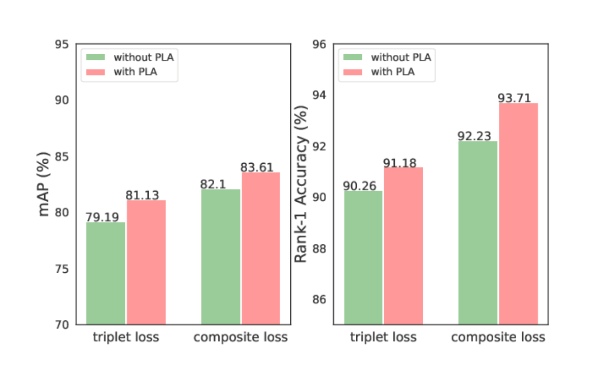
Effects on Loss Concatenation. In the proposed network structure, after global max pooling of the ResNet-50 backbone, the network is split into two heads, one for triplet loss and the other for cross-entropy loss. Considering that triplet loss is a ranking function, while cross-entropy loss is a classification target, their feature representations are different. Combining them should have richer feature representation than each of them alone. In our testing process, we used three variants of the network head: 2048-dim feature with cross-entropy loss only, 2048-dim feature with triplet loss only, and the 2048-dim feature (concatenation of two 1024-dim feature embeddings). Fig. 3 shows the effectiveness of loss concatenation on Market-1501 dataset in terms of mAP and Rank-1 accuracy. Coupling the feature concatenation method, the proposed progressive learning algorithm brought significant improvements $4.4\%$ for mAP and $3.5\%$ for Rank-1 compared to using triplet loss alone on Market-1501 dataset.

Effects on Progressive Learning. Fig. 3 shows the effectiveness of progressive learning on Market-1501 dataset. With the proposed PLA, the triplet feature embedding achieved mAP and Rank-1 accuracy of $81.1\%$ and $91.2\%$, respectively, outperforming the accuracies using each type of loss with 2048-dim feature without PLA. We found progressive learning and concatenated feature embedding, when used together, produced the best results. This indicates the progressive learning is effective to learn more accurate and robust representation of person identities.

Effectiveness on Training Convergence. To illustrate the robustness of our loss function on the convergence performance, we use the same ResNet-50 backbone as the network architecture and train it on Market1501 using two methods: 1) the proposed PLA training method; 2) batch hard training [5]. As shown in Fig. 4, the red curve shows loss values of our method, which entails two stages compared with batch hard training method shown as the blue curve. It is observed that in the first training stage (first 5,700 batches), our loss converges faster than batch hard loss as the proposed method trains easy and medium samples at the beginning. When hard samples are introduced to the proposed method, it comes to the second stage. The loss is significantly reduced further using PLA, leading to the final improvement, while the loss of hard samples cannot be reduced any more. Note that in the beginning of the second training stage, the red curve has a sudden jump because harder samples are introduced; however, the loss value gradually dropped until achieving the lowest ever one. The results illustrate that learning progressively by the level of hardness is beneficial to model convergence and achieves lower loss.

We compare the proposed ReID approach with various ReID approaches based on both global models and part models. The global model based approaches include: SVDNet [4], TriNet [5], GP-reid [21], and ResNet-50 based DaRe [9]. The part model based approaches include: HA-CNN [6], PCB [1], Aligned-ReID [29], Deep-Person [30] and MGN [2].

The comparison results over state-of-the-art methods with global models are shown in Table II. Without the reranking technique, GP-reid [21] achieved a good performance as it properly makes use of many existing techniques. The proposed PLA consistently outperforms all other global feature models by a large margin without reranking technique, except for GP-reid. PLA outperforms GP-reid in terms of mAP accuracy by $2.4\%$ and $5.6\%$ on Market-1501 dataset with single query mode and multiple query mode, respectively. However, GP-reid slightly outperforms PLA in terms of mAP and Rank-1 accuracy by $0.3\%$ and $0.9\%$, respectively, on DukeMTMC dataset. Note that in this work the learning rate schedule is uniform in all experiments and not specially tailored for DukeMTMC dataset. We can observe that the proposed PLA consistently outperforms all other methods with reranking by a large margin. PLA outperforms DaRe in terms of mAP by $9.4\%$, $5.1\%$, $7.3\%$ and $9.5\%$ without reranking on Market-1501(SQ), CUHK03(D), CUHK03(L) and DukeMTMC datasets respectively. Overall, the proposed PLA has the best performance over other global models.

Although the proposed approach is within the scope of global feature model, we also compare it with the accuracies produced by multi-branch part models, as shown in Table II for all datasets. In Table II, it is obvious that MGN achieves the highest accuracies among all part models on Market-1501 dataset without reranking technique. It is evident that the proposed PLA outperforms all previous works except for MGN. In terms of Rank-1 accuracy performance without reranking, PLA is overall comparable with MGN in terms of Rank-1 accuracy: MGN exceeds PLA by $2\%$ and $4.3\%$ on Market-1501(SQ) and DukeMTMC dataset respectively, while MGN is inferior than PLA by $0.4\%$ and $3.5\%$ on CUHK03(D) and CUHK03(L) datasets. We can also observe that with reranking, PLA outperforms DaRe by a large margin achieving the highest mAP and Rank-1 values ever publicly reported on the CUHK03(D) and CUHK03(L) datasets.

The proposed PLA is designed for resource-aware ReID, and a good trade off between accuracy and efficiency is expected. The computational cost is reported with respect to the total number of basic operations, i.e., multiplications and additions (Mul-Add), which is proportional to the actual running timing. Reranking is not included in the Mul-Add calculation. HA-CNN [6], ResNet-50 based DaRe [9], PCB(RPP) [1] and MGN [2] are chosen to be compared with the proposed PLA for their good performance.

The graph of accuracy vs. efficiency is shown in Fig. 5 (a). Accuracy reported is the average mAP on Market-1501, CUHK03(D), CUHK03(L) and DukeMTMC datasets without reranking. We observe that the proposed PLA achieves significantly higher accuracies than HA-CNN and DaRe. In particular, PLA achieves slightly higher accuracy than PCB which is a strong part model baseline for ReID, yet saving more than $30\%$ computation cost. MGN outperforms PLA and PCB in accuracy by a small margin, however, it has a tremendous Mul-Add of roughly $2.3\times 10^{10}$ which is about 3 times of PLA.

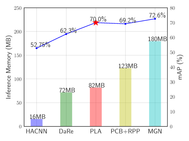
The graph of accuracy vs. inference memory is shown in Fig. 5 (b). It is evident that the trade off situation is similar to that in Fig. 5 (a). Although HA-CNN is a multi-branch part model, the input size is fairly small compared with other approaches, making it the most lightweight approach. HA-CNN shows good accuracy on Market-1501 dataset but exhibits rather low accuracies on CUHK and DukeMTMC datasets, as shown in Table II. MGN outperforms all others in terms of accuracy, but it is more than 2 times of the PLA inference memory. Accordingly, it requires at least 11.6GB memory for inference with a commonly used batch size of 64, which even cannot be loaded using GTX 1080Ti (11.17GB). Note that even though network acceleration techniques TensorRT [41] and network compression techniques can be used to save Mul-Add and reduce inference memory, respectively, for strong part models including PCB and MGN, they will also benefit PLA by similar acceleration and compression ratios since ResNet-50 is the backbone of all these networks.

It is evident that in Fig. 5, our method is outstanding in its accuracy and resource balance: the models with less resource requirements exhibit obvious lower or unstable accuracy while those with slightly higher accuracy will consume unnecessarily much more computational cost and inference memory.

References

- [1] Y. Sun, L. Zheng, Y. Yang, Q. Tian, and S. Wang, “Beyond part models: Person retrieval with refined part pooling,” arXiv preprint arXiv:1711.09349, 2017.
- [2] G. Wang, Y. Yuan, X. Chen, J. Li, and X. Zhou, “Learning discriminative features with multiple granularities for person re-identification,” in Proceedings of the 26th ACM international conference on Multimedia, 2018, pp. 274–282.
- [3] C. C.-H. Hsu, M. Y.-C. Wang, H. C. Shen, R. H.-C. Chiang, and C. H. Wen, “Fallcare+: An iot surveillance system for fall detection,” in 2017 International Conference on Applied System Innovation (ICASI). IEEE, 2017, pp. 921–922.
- [4] Y. Sun, L. Zheng, W. Deng, and S. Wang, “Svdnet for pedestrian retrieval,” in IEEE International Conference on Computer Vision, 2017, pp. 3820–3828.
- [5] A. Hermans, L. Beyer, and B. Leibe, “In defense of the triplet loss for person re-identification,” arXiv preprint arXiv:1703.07737, 2017.
- [6] W. Li, X. Zhu, and S. Gong, “Harmonious attention network for person re-identification,” in Computer Vision and Pattern Recognition, vol. 1, 2018, p. 2.
- [7] F. Schroff, D. Kalenichenko, and J. Philbin, “Facenet: A unified embedding for face recognition and clustering,” in Proceedings of the IEEE conference on computer vision and pattern recognition, 2015, pp. 815–823.
- [8] K. He, X. Zhang, S. Ren, and J. Sun, “Deep residual learning for image recognition,” in Proceedings of the IEEE conference on computer vision and pattern recognition, 2016, pp. 770–778.
- [9] Y. Wang, L. Wang, Y. You, X. Zou, V. Chen, S. Li, G. Huang, B. Hariharan, and K. Q. Weinberger, “Resource aware person re-identification across multiple resolutions,” in Proceedings of the IEEE Conference on Computer Vision and Pattern Recognition, 2018, pp. 8042–8051.
- [10] K. Q. Weinberger, J. Blitzer, and L. K. Saul, “Distance metric learning for large margin nearest neighbor classification,” in Advances in neural information processing systems, 2006, pp. 1473–1480.
- [11] H. Oh Song, Y. Xiang, S. Jegelka, and S. Savarese, “Deep metric learning via lifted structured feature embedding,” in Proceedings of the IEEE Conference on Computer Vision and Pattern Recognition, 2016, pp. 4004–4012.
- [12] S. Khamis, C.-H. Kuo, V. K. Singh, V. D. Shet, and L. S. Davis, “Joint learning for attribute-consistent person re-identification,” in European Conference on Computer Vision. Springer, 2014, pp. 134–146.
- [13] S. Ding, L. Lin, G. Wang, and H. Chao, “Deep feature learning with relative distance comparison for person re-identification,” Pattern Recognition, vol. 48, no. 10, pp. 2993–3003, 2015.
- [14] S. Paisitkriangkrai, C. Shen, and A. Van Den Hengel, “Learning to rank in person re-identification with metric ensembles,” in Proceedings of the IEEE Conference on Computer Vision and Pattern Recognition, 2015, pp. 1846–1855.
- [15] D. Cheng, Y. Gong, S. Zhou, J. Wang, and N. Zheng, “Person re-identification by multi-channel parts-based cnn with improved triplet loss function,” in Computer Vision and Pattern Recognition, 2016, pp. 1335–1344.
- [16] F. Wang, W. Zuo, L. Lin, D. Zhang, and L. Zhang, “Joint learning of single-image and cross-image representations for person re-identification,” in Computer Vision and Pattern Recognition, 2016, pp. 1288–1296.
- [17] H. Shi, Y. Yang, X. Zhu, S. Liao, Z. Lei, W. Zheng, and S. Z. Li, “Embedding deep metric for person re-identification: A study against large variations,” in European Conference on Computer Vision. Springer, 2016, pp. 732–748.
- [18] C. Su, S. Zhang, J. Xing, W. Gao, and Q. Tian, “Deep attributes driven multi-camera person re-identification,” in European Conference on Computer Vision, 2016, pp. 475–491.
- [19] W. Chen, X. Chen, J. Zhang, and K. Huang, “A multi-task deep network for person re-identification.” in AAAI, 2017, pp. 3988–3994.
- [20] H. Liu, J. Feng, M. Qi, J. Jiang, and S. Yan, “End-to-end comparative attention networks for person re-identification.” IEEE Transactions on Image Processing, vol. PP, no. 99, pp. 1–1, 2016.
- [21] J. Almazan, B. Gajic, N. Murray, and D. Larlus, “Re-id done right: towards good practices for person re-identification,” arXiv preprint arXiv:1801.05339, 2018.
- [22] D. Li, X. Chen, Z. Zhang, and K. Huang, “Learning deep context-aware features over body and latent parts for person re-identification,” in Proceedings of the IEEE Conference on Computer Vision and Pattern Recognition, 2017, pp. 384–393.
- [23] L. Zhao, X. Li, Y. Zhuang, and J. Wang, “Deeply-learned part-aligned representations for person re-identification,” in IEEE International Conference on Computer Vision, 2017, pp. 3239–3248.
- [24] C. Su, J. Li, S. Zhang, J. Xing, W. Gao, and Q. Tian, “Pose-driven deep convolutional model for person re-identification,” in IEEE International Conference on Computer Vision. IEEE, 2017, pp. 3980–3989.
- [25] W. Li, X. Zhu, and S. Gong, “Person re-identification by deep joint learning of multi-loss classification,” arXiv preprint arXiv:1705.04724, 2017.
- [26] H. Zhao, M. Tian, S. Sun, J. Shao, J. Yan, S. Yi, X. Wang, and X. Tang, “Spindle net: Person re-identification with human body region guided feature decomposition and fusion,” in Computer Vision and Pattern Recognition, 2017, pp. 907–915.
- [27] H. Yao, S. Zhang, Y. Zhang, J. Li, and Q. Tian, “Deep representation learning with part loss for person re-identification,” arXiv preprint arXiv:1707.00798, 2017.
- [28] X. Liu, H. Zhao, M. Tian, L. Sheng, J. Shao, J. Yan, and X. Wang, “Hydraplus-net: Attentive deep features for pedestrian analysis,” in Proceedings of the IEEE international conference on computer vision, 2017, pp. 1–9.
- [29] X. Zhang, H. Luo, X. Fan, W. Xiang, Y. Sun, Q. Xiao, W. Jiang, C. Zhang, and J. Sun, “Alignedreid: Surpassing human-level performance in person re-identification,” arXiv preprint arXiv:1711.08184, 2017.
- [30] X. Bai, M. Yang, T. Huang, Z. Dou, R. Yu, and Y. Xu, “Deep-person: Learning discriminative deep features for person re-identification,” arXiv preprint arXiv:1711.10658, 2017.
- [31] B. Shahriari, K. Swersky, Z. Wang, R. P. Adams, and N. De Freitas, “Taking the human out of the loop: A review of bayesian optimization,” Proceedings of the IEEE, vol. 104, no. 1, pp. 148–175, 2016.
- [32] J. Snoek, H. Larochelle, and R. P. Adams, “Practical bayesian optimization of machine learning algorithms,” in Advances in neural information processing systems, 2012, pp. 2951–2959.
- [33] Z. Zhong, L. Zheng, D. Cao, and S. Li, “Re-ranking person re-identification with k-reciprocal encoding,” in IEEE Conference on Computer Vision and Pattern Recognition, 2017, pp. 3652–3661.
- [34] L. Zheng, L. Shen, L. Tian, S. Wang, J. Wang, and Q. Tian, “Scalable person re-identification: A benchmark,” in Proceedings of the IEEE International Conference on Computer Vision, 2015, pp. 1116–1124.
- [35] E. Ristani, F. Solera, R. Zou, R. Cucchiara, and C. Tomasi, “Performance measures and a data set for multi-target, multi-camera tracking,” in European Conference on Computer Vision workshop on Benchmarking Multi-Target Tracking, 2016.
- [36] W. Li, R. Zhao, T. Xiao, and X. Wang, “Deepreid: Deep filter pairing neural network for person re-identification,” in Proceedings of the IEEE Conference on Computer Vision and Pattern Recognition, 2014, pp. 152–159.
- [37] C. Mao, Y. Li, Z. Zhang, Y. Zhang, and X. Li, “Pyramid person matching network for person re-identification,” in The Ninth Asian Conference on Machine Learning, 2017, pp. 487–497.
- [38] Y. Suh, J. Wang, S. Tang, T. Mei, and K. M. Lee, “Part-aligned bilinear representations for person re-identification,” in Proceedings of the European Conference on Computer Vision (ECCV), September 2018.
- [39] Z. Zhong, L. Zheng, G. Kang, S. Li, and Y. Yang, “Random erasing data augmentation,” arXiv preprint arXiv:1708.04896, 2017.
- [40] D. P. Kingma and J. Ba, “Adam: A method for stochastic optimization,” arXiv preprint arXiv:1412.6980, 2014.
- [41] NVIDIA, “NVIDIA TensorRT: Programmable Inference Accelerator,” https://developer.nvidia.com/tensorrt, 2018.