\msmlauthor

Andreas Mardt¹¹ 1 equal contribution and Luca Pasquali¹¹ 1 equal contribution
Freie Universität Berlin, Department of Mathematics and Computer Science, Arnimallee 6, 14195 Berlin, Germany and Frank Noé
Freie Universität Berlin, Department of Mathematics and Computer Science, Arnimallee 6, 14195 Berlin, Germany
Freie Universität Berlin, Department of Physics, Arnimallee 6, 14195 Berlin, Germany
Rice University, Department of Chemistry, Houston TX, 77005, United States and Hao Wu
Tongji University, School of Mathematical Sciences, Shanghai, 200092, P.R. China

Deep learning Markov and Koopman models with physical constraints

Abstract

The long-timescale behavior of complex dynamical systems can be described by linear Markov or Koopman models in a suitable latent space. Recent variational approaches allow the latent space representation and the linear dynamical model to be optimized via unsupervised machine learning methods. Incorporation of physical constraints such as time-reversibility or stochasticity into the dynamical model has been established for a linear, but not for arbitrarily nonlinear (deep learning) representations of the latent space. Here we develop theory and methods for deep learning Markov and Koopman models that can bear such physical constraints. We prove that the model is an universal approximator for reversible Markov processes and that it can be optimized with either maximum likelihood or the variational approach of Markov processes (VAMP). We demonstrate that the model performs equally well for equilibrium and systematically better for biased data compared to existing approaches, thus providing a tool to study the long-timescale processes of dynamical systems.

keywords

Markov state model, Koopman model, phsyical constraints, deep learning, dynamical systems

1 Introduction

Markovian, or linear dynamical models are very successful in describing the effective or long-term dynamics of complex dynamical systems, such as molecular dynamics (MD) Schütte et al. 1999; Noé et al. 2007; Swope et al. 2004; Chodera et al. 2007; Prinz et al. 2011b; Chodera and Noé 2014, wireless communications Konrad et al. 2001; Ma et al. 2001, and fluid dynamics Schmid 2010; Mezić 2013; Tu et al. 2014; Froyland et al. 2016. The cornerstone of modeling complex nonlinear dynamics with a linear and often low-dimensional model, such as a Markovian transition matrix, is that the dynamics can be linearized in the space of eigenfunctions or singular functions of the corresponding full-space dynamical operator Schütte et al. 1999; Mezić 2005; Wu and Noé 2019. In stochastic systems, such a linear model is often called Markov model, as it is convenient to describe the long-time dynamics as a Markov chain or Markov jump process between discrete states, whereas it is often called Koopman model in complex dynamical systems analysis or fluid dynamics. Markov models and Koopman models greatly simplify analysis of the dynamical systems when compared to models with explicit memory terms.

A wide variety of such linear dynamical models has been developed across different fields, including Markov State Models (MSMs) Schütte et al. 1999; Prinz et al. 2011b; Bowman et al. 2014, Markov transition models Wu and Noé 2015, Ulam’s Galerkin method Dellnitz et al. 2001; Bollt and Santitissadeekorn 2013; Froyland et al. 2014, blind-source separation Molgedey and Schuster 1994; Ziehe and Müller 1998, the variational approach for conformational dynamics (VAC) Noé and Nüske 2013; Nüske et al. 2014, time-lagged independent component analysis (TICA) Perez-Hernandez et al. 2013; Schwantes and Pande 2013, dynamic mode decomposition (DMD) Rowley et al. 2009; Schmid 2010; Tu et al. 2014, extended dynamic mode decomposition (EDMD) Williams et al. 2015, variational Koopman models Wu et al. 2017, variational diffusion maps Boninsegna et al. 2015, kinetic maps Noé and Clementi 2015; Noé et al. 2016, the variational approach of Markov processes (VAMP) Wu et al. 2017, sparse identification of nonlinear dynamics Brunton et al. 2016 and corresponding kernel embeddings Harmeling et al. 2003; Schwantes and Pande 2015; Song et al. 2013 and tensor formulations Nüske et al. 2016; Schütte and Klus 2016. All these models approximate the Markov dynamics through a linear model:

\mathbb{E}[(\mathbf{g}(\mathbf{x}_{t+\tau})]=\mathbf{K}^{T}\mathbb{E}[\mathbf{f}(\mathbf{x}_{t})]

(1)

where $\mathbf{f},\mathbf{g}$ transform the configuration $\mathbf{x}$ into a latent space representation in which the dynamics are linear, usually the space of slow transitions or rare events Noé and Clementi 2017. $\mathbf{K}$ is an MSM transition matrix, or a Koopman model, and can be interpreted as a finite-rank approximation of the full-dimensional dynamical Markov operator Schütte et al. 1999; Koopman 1931; Mezić 2005; Wu and Noé 2019.

MSMs have been particularly successful as methods to extract the long-timescale kinetics from high-throughput MD simulation data, e.g. of protein dynamics Bowman et al. 2009; Prinz et al. 2011b; Buch et al. 2011; Shukla et al. 2014; Silva et al. 2014; Reubold et al. 2015; Plattner et al. 2017. In recent years, the MD community has seen a rapid increase in the available amount of simulated data of complex molecular systems due to advances in both computing power and simulation techniques Lindorff-Larsen et al. 2011; Plattner et al. 2017; Kohlhoff et al. 2014; Doerr et al. 2016. Unlike experiments, MD simulations can resolve structure and dynamics simultaneously. The extraction of kinetic, i.e. long-timescale information from simulation data, however, is not trivial, since kinetic information cannot be inferred from structural similarity Keller et al. 2010; Krivov and Karplus 2004; Nüske et al. 2014, as similar structures may be separated by high energy barriers.

Whereas MSM construction has previously been a relatively complex pipeline of feature selection, dimension reduction, clustering, estimating the transition matrix $\mathbf{K}$ , etc, these choices have recently been guided by variational approaches Noé and Nüske 2013; Nüske et al. 2014; Schwantes and Pande 2013; Perez-Hernandez et al. 2013; Wu and Noé 2019; Mardt et al. 2018; Chen et al. 2019. These variational methods aim to approximate the leading eigenfunctions or singular functions of the Markov process, which parametrize the long-time kinetics, and in which approximately linear Markovian models (1) can be obtained. Mardt et al. 2018 recently proposed VAMPnet that simultaneously learns neural networks for the latent space representations $\mathbf{f}$ and $\mathbf{g}$ as well as the transition matrix $\mathbf{K}$ in a single end-to-end learning framework. VAMPnet uses the variational approach of Markov processes (VAMP) Wu and Noé 2019 in order to optimally find $\mathbf{f}$ and $\mathbf{g}$ . The VAMPnet framework has been further developed, for example for learning directly the eigenfunctions of the Markov operator rather than the MSM transition matrix Chen et al. 2019, and for transferring parameters across chemical space Xie et al. 2019.

By means of their ability to represent very nonlinear latent space representations, VAMPnets have been demonstrated to learn high-quality MSMs with little input from human experts Mardt et al. 2018. However, there is an important aspect that is well established with “shallow” manually constructed MSMs and is yet unsolved with deep learning methods for MSMs such as VAMPnets: the incorporation of physical constraints into the transition matrix $\mathbf{K}$ , especially reversibility (detailed balance) and stochasticity.

A dynamical system is statistically reversible when the absolute (unconditional) probability of finding a transition from point $\mathbf{x}$ at time $t$ to point $\mathbf{y}$ at time $t+\tau$ is equal to the reverse. Physically, this occurs when the system, e.g. molecule is simulated in equilibrium, i.e. without applying external forces. Consequences of statistical reversibility are that (i) there is no probability flux in cycles, consistent with the second law of thermodynamics stating that no work can be extracted from a system purely driven by thermal energy, (ii) $\mathbf{K}$ can be symmetrized with an equilibrium vector and thus (iii) the transition matrix $\mathbf{K}$ has real eigenvalues. If $\mathbf{K}$ is a stochastic transition matrix, this means that it fulfills detailed balance with respect to its equilibrium vector. Even if the underlying MD system has been simulated in equilibrium, estimating a VAMPnet from finite data will not guarantee a reversible model $\mathbf{K}$ . For standard MSMs, maximum likelihood estimators have been developed to enforce reversibility Noé 2008; Bowman et al. 2009; Trendelkamp-Schroer and Noé 2013; Trendelkamp-Schroer et al. 2015. Chen et al. 2019 approached the problem by symmetrizing the covariance matrices involved in the estimation of $\mathbf{K}$ , which works well for long simulation trajectories, but introduces significant bias for many short trajectories emerging from a non-equilibrium distribution. As indicated in Mardt et al. 2018, reversible VAMPnets could be developed by using the Koopman reweighting method proposed in Wu et al. 2017, however that approach reduces the bias at a cost of a quite large estimator variance. Here we develop a new deep learning framework for Markov processes that can learn reversible transition models from non-equilibrium data in a robust and end-to-end manner.

Furthermore, a transition matrix $\mathbf{K}$ estimated via a VAMPnet is not automatically a stochastic matrix. Even when the VAMPnet encoders map to a state assignment, e.g. by using a SoftMax output Mardt et al. 2018, the transition matrix will have probability mass conservation, i.e. row sums equal 1, but may still have negative elements. With such a Markov model we can compute valid observables, such as propagated probability vectors, a valid equilibrium distribution and meaningful correlation functions. But the individual matrix elements of $\mathbf{K}$ can no longer be interpreted as transition probabilities or rates and therefore some analyses, such as transition path theory W. E and E. Vanden-Eijnden 2006; Metzner et al. 2009; Noé et al. 2009, are no longer applicable. The deep learning framework for Markov processes introduced here can optionally enforce the $\mathbf{K}$ matrix to be a stochastic matrix.

In summary, our contributions are as follows:

1.

We develop a flexible deep learning framework for Markov processes, in which deep networks can be used to learn the latent space representation of the system and a linear model $\mathbf{K}$ is learned to describe the time propagation in latent space.
2.

We develop a way to enforce $\mathbf{K}$ to be reversible or non-reversible, optionally. We proove that when enforcing reversibility we obtain a universal approximator for reversible Markov processes.
3.

We develop a way to optionally enforce $\mathbf{K}$ to be stochastic, i.e. have nonnegative elements. We can combine both physical constraints in either way, obtaining four choosable combinations of reversible/non-reversible and stochastic/non-stochastic VAMPnets or deep MSMs.
4.

We provide two optimization targets for our method, using maximum likelihood or VAMP as a loss function, and demonstrate that they provide asymptotically unbiased results.
5.

We illustrate our learning method on benchmark data and demonstrate that it yields accurate estimates in both the limit of single long simulation trajectories and many short trajectories, whereas other methods fail in the latter case.

2 Theory

2.1 Markov processes, spectral decomposition and Koopman theory

The dynamics of a Markovian dynamical system can be modeled by the transition density, i.e. the probability density to transition to a state space point $\mathbf{y}$ at time $t+\tau$ , given that the system was at state $\mathbf{x}$ at time $t$ :

p_{\tau}(\mathbf{x},\mathbf{y})=\mathbb{P}(\mathbf{x}_{t+\tau}=\mathbf{y}\mid\mathbf{x}_{t}=\mathbf{x}).

Based on the transition density, we can characterize the time evolution of the ensemble of system states as

p_{t+\tau}(\mathbf{y})=\left(\mathcal{P}_{\tau}p_{t}\right)(\mathbf{y})\triangleq\int p_{\tau}(\mathbf{x},\mathbf{y})\>p(\mathbf{x})\>\mathrm{d}\mathbf{x}

where $p_{t}$ is the probability density of the system being in any state at time $t$ and the lag time $\tau$ is the time resolution of the model. The propagation of general observable functions $f$ can be modeled as

\mathbb{E}[f(\mathbf{x}_{t+\tau})|\mathbf{x}_{t}=\mathbf{x}]=\left(\mathcal{K}_{\tau}f\right)(\mathbf{x})\triangleq\int p_{\tau}(\mathbf{x},\mathbf{y})\>f(\mathbf{y})\>\mathrm{d}\mathbf{y}.

The integral operators $\mathcal{P_{\tau}}$ and $\mathcal{K}_{\tau}$ are called propagator and Koopman operator respectively, and are both able to fully describe the Markovian dynamics. From hereon, we only consider the Koopman operator based modeling formalism, which is commonly used in the field of dynamical systems (see e.g., Mezić 2005), but all conclusions in this paper can be equivalently established by using the propagator description.

The Koopman operator is linear but infinite-dimensional, and we can generally approximate the essential part of the dynamics at long timescales by a finite-dimensional linear model in the form of Eq. (1) with $\mathbf{f}$ and $\mathbf{g}$ being two sets of latent variables. Denoting by $\rho_{0}$ the empirical distribution of $\mathbf{x}_{t}$ and $\rho_{1}$ the empirical distribution of $\mathbf{x}_{t+\tau}$ in all transition pairs $(\mathbf{x}_{t},\mathbf{x}_{t+\tau})$ , it can be proven that an optimal finite-rank approximation of the transition density can be written in the form

\hat{p}_{\tau}(\mathbf{x},\mathbf{y})=\mathbf{f}(\mathbf{x})^{\top}\mathbf{S}\mathbf{g}(\mathbf{y})\rho_{1}(\mathbf{y}),

(2)

where $\mathbf{S}=\mathbf{K}\left(\mathbb{E}[\mathbf{g}(x_{t+\tau})\mathbf{g}(x_{t+\tau})^{T}]\right)^{-1}$ Wu and Noé 2019. Based on conformation dynamics theory Schütte et al. 1999, Koopman theory Mezić 2005; Koopman 1931, and the variational approach of Markov processes (VAMP) Wu and Noé 2019, the finite-dimensional model can accurately capture the essential or long-time part of the dynamics by selecting $\mathbf{f},\mathbf{g}$ to be the dominant singular functions or eigenfunctions of the Koopman operator. Specifically, if we consider the modeling error of the Koopman operator in the sense of Hilbert-Schmidt norm, the optimal model can be given by the truncated singular value decomposition of the transition density

p_{\tau}(\mathbf{x},\mathbf{y})\approx\sum_{i=1}^{k}\sigma_{i}\psi_{i}(\mathbf{x})\phi_{i}(\mathbf{y})\rho_{1}(\mathbf{y}),

(3)

where $(\sigma_{1},\ldots,\sigma_{k})$ are the largest singular values of the Koopman operator $\mathcal{K}_{\tau}$ , $(\psi_{1},\ldots,\psi_{k})$ and $(\phi_{1},\ldots,\phi_{k})$ are the corresponding dominant left and right singular functions, and the equality holds exactly if $k\to\infty$ .

If we further assume that the dynamics are statistically reversible, which implies that the system does not contain net cycles and there is no work produced in equilibrium, then the detailed balance condition

\mu(\mathbf{x})p_{\tau}(\mathbf{x},\mathbf{y})=\mu(\mathbf{y})p_{\tau}(\mathbf{y},\mathbf{x}),

(4)

is satisfied, where $\mu(\mathbf{x})$ is the equilibrium distribution of system states. This means that the unconditional probability to observe the transition $\mathbf{x}\rightarrow\mathbf{y}$ is equal to that of transition $\mathbf{y}\rightarrow\mathbf{x}$ . In this case, the Koopman operator is a self-adjoint operator, and the truncated singular value decomposition of the dynamics is equivalent to the truncated eigendecomposition

p_{\tau}(\mathbf{x},\mathbf{y})\approx\sum_{i=1}^{k}\lambda_{i}\varphi_{i}(\mathbf{x})\varphi_{i}(\mathbf{y})\mu(\mathbf{y})

with eigenfunctions $\varphi_{i}=\psi_{i}=\phi_{i}$ and eigenvalues $\lambda_{i}=\sigma_{i}$ when the equilibrium is achieved by data.

The eigenvalues and eigenfunctions can be systematically approximated from data by invoking the variational approach of conformation dynamics (VAC) Nüske et al. 2014; Mardt et al. 2018; Wu and Noé 2019, which provides a loss function with which hyper-parameter selection can be made in the traditional MSM construction pipeline McGibbon and Pande 2015, and which can be used in order to train a deep neural network to represent the eigenfunctions Chen et al. 2019. Likewise, the singular values and singular functions of non-reversible or even non-stationary dynamical models can be variationally approximated with VAMP Wu and Noé 2019, which in turn can be used for hyper-parameter selection in MSM pipelines Scherer et al. 2019 and deep learning molecular kinetics with VAMPnets Mardt et al. 2018.

In this paper, we will also use neural networks as universal function approximators to find latent variables with a suitable optimization principle. The main novelty is that our framework allows to obtain a finite-dimensional model that incorporates desired physical constraints such as stochasticity and reversibility in an asymptotically unbiased way.

3 Deep Markov Model with physical constraints

3.1 Transition Model

The aim of this section is to construct a general model which approximates the Markovian process defined by the transition density; this density can be learned with neural networks and physical constraints for reversibility and stochasticity of the transition matrix can be built into it. We propose the following model of the transition density:

p_{\tau}(\mathbf{x},\mathbf{y})=\boldsymbol{\chi}(\mathbf{x})^{T}\mathbf{S}\boldsymbol{\chi}(\mathbf{y})\boldsymbol{\chi}(\mathbf{y})^{T}\mathbf{u}\rho_{1}(\mathbf{y}),

(5)

which is a special representation of the general finite-dimensional model (2-3) with the choices $\mathbf{f}(\mathbf{x})=\boldsymbol{\chi}(\mathbf{x})$ and $\mathbf{g}(\mathbf{y})=\boldsymbol{\chi}(\mathbf{y})\boldsymbol{\chi}(\mathbf{y})^{T}\mathbf{u}$ . However, we will demonstrate that this choice leads to an universal approximator for the Markov processes of interest. Here, $\boldsymbol{\chi}$ is a neural network that maps a sample $\mathbf{x}$ from configuration space onto a fuzzy clustering, which can be thought of indicating to what degree $\mathbf{x}$ belongs to each of the few metastable states. The trainable vector $\mathbf{u}$ is necessary to reweight the empirical distribution towards the equilibrium distribution of the system. Eq. (5) can be understood as mapping the starting sample $\mathbf{x}$ to the state representation $\boldsymbol{\chi}(\mathbf{x})$ , making a time propagation with $\mathbf{S}$ , and checking how close it ends up to the state representation $\boldsymbol{\chi}(\mathbf{y})$ , which is weighted with respect to the system’s equilibrium probability (Fig. 1).

Figure 1: Schematic of the proposed deep learning architecture for Markov processes with physical constraints. For each time step

t

of the training data, the coordinates

\mathbf{x}_{t}

and

\mathbf{x}_{t+\tau}

are passed to two instances of the same network

\boldsymbol{\chi}

. The transformed outputs are then concatenated, and used together with the trainable variables

\mathbf{S},\mathbf{u}

to obtain an estimate of the transition density

p(\mathbf{y}=\mathbf{x}_{t+\tau}\mid\mathbf{x}=\mathbf{x}_{t}).

This probability estimate allows us to train

\boldsymbol{\chi},\mathbf{S},\mathbf{u}

using a Maximum Likelihood loss. Alternatively, the whole architecture can be trained using as an optimization target the VAMP-E score. The scheme is similar to a classical VAMPnet Mardt et al. 2018, but has the ability to build in physical constraints such as reversibility and stochasticity into the parameters

\mathbf{S},\mathbf{u}

Here we work with stationary dynamical systems and thus assume that there exists a unique equilibrium distribution $\mu(\mathbf{x})=\mathbf{u}^{T}\boldsymbol{\chi}(\mathbf{x})\rho(\mathbf{x})$ . Hence our model needs to always fulfill the following constraints to guarantee a normalized equilibrium and transition density (see Appendix 9.1 for proof):

1.

Normalization of state assignment: $\boldsymbol{\chi}(\mathbf{x})^{T}\mathbf{1}=1.$
2.

Normalization of the reweighting vector: $\bar{\boldsymbol{\chi}}^{T}\mathbf{u}=1$ , where $\bar{\boldsymbol{\chi}}=\mathbb{E}\left[\boldsymbol{\chi}(\mathbf{x}_{t+\tau})\right]$ is the empirical state probability.
3.

Normalization of transition density: $\mathbf{S}\mathbf{C}_{\tau\tau}^{\prime}\mathbf{u}=\mathbf{1}$ where $\mathbf{C}_{\tau\tau}^{\prime}=\mathbb{E}\left[\boldsymbol{\chi}(\mathbf{x}_{t+\tau})\boldsymbol{\chi}(\mathbf{x}_{t+\tau})^{\top}\right]$ is the empirical covariance matrix of $\boldsymbol{\chi}(\mathbf{x}_{t+\tau})$ . As a result the Koopman matrix preserves probability mass by means of $\mathbf{K1}=\mathbf{\mathbf{S}\mathbf{C}_{\tau\tau}^{\prime}\mathbf{u}=\mathbf{1}}$ .

By substituting the equilibrium distribution $\mu(\mathbf{x})$ into (5), the finite-dimensional model proposed in this section can be rewritten as

p_{\tau}(\mathbf{x},\mathbf{y})=\boldsymbol{\chi}(\mathbf{x})^{T}\mathbf{S}\boldsymbol{\chi}(\mathbf{y})\mu(\mathbf{y}).

(6)

So the equilibrium Koopman matrix $\mathbf{K}$ acts as:

\mathbb{E}[\boldsymbol{\chi}(\mathbf{x}_{t+\tau})]=\mathbf{K}^{\top}\mathbb{E}[\boldsymbol{\chi}(\mathbf{x}_{t})],

and can be estimated from:

\displaystyle\mathbf{K}

\displaystyle=\mathbf{S\boldsymbol{\Sigma}}

(7)

with

	$\displaystyle\boldsymbol{\Sigma}$	$\displaystyle=\int\boldsymbol{\chi}(\mathbf{y})\mu(\mathbf{y})\boldsymbol{\chi}(\mathbf{y})^{T}\mathrm{d}\mathbf{y}$
		$\displaystyle=\int\boldsymbol{\chi}(\mathbf{y})\rho_{1}(\mathbf{y})\boldsymbol{\chi}(\mathbf{y})^{T}\mathbf{u}\boldsymbol{\chi}(\mathbf{y})^{T}\mathrm{d}\mathbf{y}$		(8)

being the equilibrium covariance matrix of $\boldsymbol{\chi}$ . See Appendix 9.4 for an overview of the relationship with traditional MSMs.

3.2 Reversible deep Markov Model

In addition to the necessary constraints introduced above, we have the choice of enforcing further physical constraints. In order to enforce detailed balance (4), or statistical reversibility, into the model, we enforce:

\mathbf{S}=\mathbf{S}^{T}

(9)

Proof of reversibility

Inserting (9) into (5) leads to the detailed balance equation 4.

	$\displaystyle\mu(\mathbf{x})p_{\tau}(\mathbf{x},\mathbf{y})$	$\displaystyle=\mathbf{u}^{T}\boldsymbol{\chi}(\mathbf{x})\rho(\mathbf{x})\boldsymbol{\chi}(\mathbf{x})^{T}\mathbf{S}\boldsymbol{\chi}(\mathbf{y})\rho(\mathbf{y})\boldsymbol{\chi}(\mathbf{y})^{T}\mathbf{u}$
		$\displaystyle=\mu(\mathbf{y})p_{\tau}(\mathbf{y},\mathbf{x}).$

Therefore, the Markov process defined by $p_{\tau}(\mathbf{x},\mathbf{y})$ is a reversible Markov process with stationary distribution $\mu(\mathbf{x})$ .

3.3 Reversible deep MSM

The mandatory constraints above already enforce $\sum_{j}k_{ij}=1$ for all $i$ with $k_{ij}$ denoting the $(i,j)$ -th element of $\mathbf{K}$ , and hence probability mass conservation. In order to force the Koopman matrix $\mathbf{K}$ to be a stochastic Markov chain matrix, we additionally need to achieve non-negative elements:

\displaystyle k_{ij}

\displaystyle\geq 0\>\>\>\>\forall i,j

(10)

This can be enforced by the additional constraints:

\text{All elements of }\mathbf{u},\mathbf{S},\text{ and }\boldsymbol{\chi}\text{ are non-negative.}

(11)

The non-negativity (10) directly follows from (7-8), since all factors are positive.

Additionally, constraint (11) ensures that the full transition density is a real probability density, i.e. $p_{\tau}(\mathbf{x},\mathbf{y})\geq 0$ $\forall\mathbf{x},\mathbf{y}$ . However, this condition may be violated when using a finite rank approximation of a Koopman model Wu and Noé 2019.

3.4 Choosing physical constraints

By toggling the two optional physical constraints, reversibility and stochasticity, we can change the class of Markov Model we want to build:

1.

Non-reversible VAMPnet (VAMPnet): This is the most general case, where both optional constraints are not enforced. This grants the model the highest flexibility to approximate the Koopman operator. Hence the model will obtain the best approximation of the eigenfunctions of the Koopman operator. It can be understood as an alternative approach to VAMPnets Mardt et al. 2018, where the proposed model learns a reweighting vector and the Koopman matrix via additional parameters.
2.

Non-reversible deep MSM (DMSM): If we obey the non-negativity constraints (Eq. 11), we obtain a model with a stochastic transition matrix $\mathbf{K}$ and a nonnegative transition density $p_{\tau}(\mathbf{x},\mathbf{y})$ . A DMSM can be viewed as a special case of the general deep MSM Wu et al. 2018 with $\mathbf{q}(\mathbf{y})=\mathbf{S}\boldsymbol{\chi}(\mathbf{y})\rho(\mathbf{y})\boldsymbol{\chi}(\mathbf{y})^{T}\mathbf{u},$ where $q_{i}(\mathbf{y})$ is the probability of jumping to configuration $\mathbf{y}$ when starting from state $i$ .
3.

Reversible VAMPnet (RevVAMPnet): Activating the reversibility constraint (Eq. 9) results in a reversible transition density with respect to the equilibrium distribution $\mu$ .
4.

Reversible deep MSM (RevDMSM): The last model combines both constraints (Eq. 9 & 11) to ensure a reversible model and a stochastic transition matrix. Such a model is desirable when seeking a reversible dynamical model that should be analyzed with algorithms operating on individual transition probabilities, such as transition path theory or committor analyses. To the best knowledge of the authors no algorithm exists to train a neural network framework which results in such a model.

Since for the first two models results are already reported, we will focus in our analysis on the latter two models.

Symmetrized VAMPnet

(SymVAMPnet)

We compare our reversible models to a previously proposed model Chen et al. 2019; Wu et al. 2017, which estimates a VAMPnet but additionally enforces reversibility by symmetrizing the correlation matrices entering the VAMP score as follows:

	$\displaystyle\mathbf{C}_{00}$	$\displaystyle=\frac{1}{2}(\mathbb{E}[\boldsymbol{\chi}(\mathbf{x}_{t})\boldsymbol{\chi}(\mathbf{x}_{t})^{T}]+\mathbb{E}[\boldsymbol{\chi}(\mathbf{x}_{t+\tau})\boldsymbol{\chi}(\mathbf{x}_{t+\tau})^{T}]),$
	$\displaystyle\mathbf{C}_{01}$	$\displaystyle=\frac{1}{2}(\mathbb{E}[\boldsymbol{\chi}(\mathbf{x}_{t})\boldsymbol{\chi}(\mathbf{x}_{t+\tau})^{T}]+\mathbb{E}[\boldsymbol{\chi}(\mathbf{x}_{t+\tau})\boldsymbol{\chi}(\mathbf{x}_{t})^{T}]),$
	$\displaystyle\mathbf{C}_{11}$	$\displaystyle=\mathbf{C}_{00}.$

In the limit of a long equilibrium simulation, this model is asymptotically unbiased, but it can be subject to a strong bias in the case of short simulations starting from a non-equilibrium distribution, which is the main application scenario of Markov modeling (see also Wu et al. 2017).

4 Machine Learning Architecture and Algorithm

4.1 Loss function

For training the model two learning objectives can be used, the VAMP-E score Wu and Noé 2019 and maximum likelihood (ML), respectively. In the case of ML we can directly estimate the likelihood to observe all the data pairs $(\mathbf{x}_{t},\mathbf{x}_{t+\tau})$ in the trajectory according to the transition density (5):

\log(L)=\log(\prod_{t=1}^{T-\tau}p_{\tau}(\mathbf{x}_{t},\mathbf{x}_{t+\tau}))=\sum_{t=1}^{T-\tau}\log(p_{\tau}(\mathbf{x}_{t},\mathbf{x}_{t+\tau})).

In order to use ML training, it is necessary that $p_{\tau}(\mathbf{x},\mathbf{y})\geq 0$ , which is exclusively the case for the non-reversible and reversible MSM, i.e. when enforcing constraint (11).

If we consider the VAMP-E score, we can rewrite:

p_{\tau}(\mathbf{x},\mathbf{y})=\boldsymbol{\chi}(\mathbf{x})^{T}\mathbf{S}\boldsymbol{\gamma}(\mathbf{y})\rho(\mathbf{y}),

with

\boldsymbol{\gamma}(\mathbf{x})=\boldsymbol{\chi}(\mathbf{x})\boldsymbol{\chi}(\mathbf{x})^{T}\mathbf{u},

which is a weighted state representation compensating for non-equilibrium data. The corresponding VAMP-E score to be maximized is then

R=\mathrm{tr}[\mathbf{S}^{T}\mathbf{C_{\chi\chi}\mathbf{S}}\mathbf{C}_{\gamma\gamma}-2\mathbf{S}^{T}\mathbf{C}_{\chi\gamma}],

where

	$\displaystyle\mathbf{C}_{\chi\chi}$	$\displaystyle=\mathbb{E}[\boldsymbol{\chi}(\mathbf{x}_{t})\boldsymbol{\chi}(\mathbf{x}_{t})^{T}],$
	$\displaystyle\mathbf{C}_{\chi\gamma}$	$\displaystyle=\mathbb{E}[\boldsymbol{\chi}(\mathbf{x}_{t})\boldsymbol{\gamma}(\mathbf{x}_{t+\tau})^{T}],$
	$\displaystyle\mathbf{C}_{\gamma\gamma}$	$\displaystyle=\mathbb{E}[\boldsymbol{\gamma}(\mathbf{x}_{t+\tau})\boldsymbol{\gamma}(\mathbf{x}_{t+\tau})^{T}].$

This score can be employed for all four different model classes and is the only score we consider to train the Koopman models.

4.2 Enforcing physical constraints

Using either loss function, we have to fulfill the constraints by parameterizing $\mathbf{S}$ and $\mathbf{u}$ . First we consider $\mathbf{u}$ . If we choose arbitrary weights $\mathbf{w}^{\text{u}}$ , we can enforce the non-negativity by squeezing the weights through an exponential and enforce $\bar{\boldsymbol{\chi}}^{\top}\mathbf{u}=1$ by proper normalization:

\mathbf{u}=\frac{\exp(\mathbf{w}^{\text{u}})}{\bar{\boldsymbol{\chi}}^{\top}\exp(\mathbf{w}^{\text{u}})}.

For $\mathbf{S}$ we have arbitrary weights $\mathbf{W}^{\text{S}}$ . The symmetry and non-negativity are enforced via:

	$\displaystyle\mathbf{W}_{1}$	$\displaystyle=\sigma(\mathbf{W}^{\text{S}})+\sigma(\mathbf{W}^{\text{S}^{T}})$
	$\displaystyle\sigma(x)$	$\displaystyle=\begin{cases}\exp(x)&,\text{ if }x<0\\ x+1&,\text{ otherwise}\end{cases}.$

In addition, we need to take care of $\mathbf{S}\mathbf{C}_{\tau\tau}^{\prime}\mathbf{u}=\mathbf{Sv}=\mathbf{1}$ . In order to not reverse the symmetry, we can still change the diagonal elements via $\mathbf{w_{2}}$ .

	$\displaystyle\mathbf{S}$	$\displaystyle=\mathbf{W}_{1}+\text{diag ($\mathbf{w_{2}}$)}$
	$\displaystyle(\mathbf{Sv})_{i}$	$\displaystyle=\sum_{k}W_{ik}v_{k}+w_{i}v_{i}$
	$\displaystyle\Rightarrow w_{i}$	$\displaystyle=\frac{1-\sum_{k}W_{ik}v_{k}}{v_{i}}.$

Since the expression could result into negative elements for $\mathbf{S}$ , we need to normalize $\mathbf{W}_{1}$ beforehand, optimally by $||\mathbf{W}_{1}\mathbf{v}||_{\inf}$ . Any function which returns a value larger than the maximum norm can be used, although it should be differentiable for gradient based optimization methods; furthermore, the choice strongly influences the training properties, as if the value is not a good approximation of the maximum norm $\mathbf{S}$ will be dominated by the diagonal elements and thus harder to train. All the p-norms fulfill the requirements, and the higher the order the closer to the maximum norm they will be; we considered $p=20$ to be an acceptable value.

4.3 Training algorithm

1.

Train a VAMPnet with SoftMax output as the $\boldsymbol{\chi}$ function with VAMP-2
2.

Train $\mathbf{S}$ and $\mathbf{u}$ while keeping $\boldsymbol{\chi}$ fixed with VAMP-E score or ML with the whole training set in one batch
3.

Train everything with VAMP-E or ML
4.

For the implied timescales keep $\boldsymbol{\chi}$ fixed and train only for $\mathbf{S}$ and $\mathbf{u}$ with the whole training set in one batch.

The first two steps are included to stabilize the training, but are in principle not necessary. The training might be further stabilized by setting $\mathbf{u}$ to its optimal value for a given $\boldsymbol{\chi}$ calculated via a non-reversible Koopman $\mathbf{K_{\mathrm{non}}}$ model and the stationary distribution $\boldsymbol{\pi}=\boldsymbol{\pi}\mathbf{K_{\mathrm{non}}}$ as

\mathbf{u=\mathbf{C_{\chi\chi}^{-1}}}\boldsymbol{\pi},

which can be repeated during the training process, where $\mathbf{u}$ must still fulfill the non-negative constraint.

5 Deep reversible Markov Models are universal approximators for reversible Markov processes

In order to show that our model is flexible enough to approximate any reversible Markov process, we will proove that the proposed model is a universal approximator for reversible Markov processes. The non-reversible case was treated earlier by Mardt et al. 2018, and we therefore do not focus on it here. (see Appendices 9.2 and 9.3 for proofs)

Proposition 1. For a reversible Markov process $\{\mathbf{x}_{t}\}$ with Koopman operator $\mathcal{K_{\tau}}$ , if there are constants $C_{0},C_{1}$ , so that

	$\displaystyle\rho_{0}(\mathbf{x})\mu(\mathbf{x})^{-1}$	$\displaystyle\leq C_{0},$
	$\displaystyle\rho_{1}(\mathbf{x})^{-1}\mu(\mathbf{x})$	$\displaystyle\leq C_{1}$

for any $\mathbf{x}$ , the Koopman operator $\mathcal{\hat{K_{\tau}^{*}}}$ of the optimal (d+1)-dimensional model in the form of (5) with the largest VAMP-E score satisfies

||\mathcal{\hat{K_{\tau}^{*}}-\mathcal{K_{\tau}}||{}_{\mathrm{HS}}^{\mathrm{2}}}\leq C_{0}C_{1}\sum_{i=d+1}^{\infty}\lambda_{i}^{2},

where $\mu$ is the stationary density, and $\lambda_{i}$ denotes the i-th largest eigenvalue of $\mathcal{K_{\tau}}$ .

The following proposition shows that in equilibrium we can identify the dominant eigencomponents with our model.

Proposition 2. If $\{\mathbf{x}_{t}\}$ is a reversible and stationary Markov process with Koopman operator $\mathcal{K_{\tau}}$ , the VAMP-E score $\mathcal{R}_{E}$ of the proposed model with $\mathrm{dim}(\boldsymbol{\chi})=d$ satisfies

\mathcal{R}_{E}\leq\sum_{i=1}^{d}\lambda_{i}^{2},

(12)

and the equality can hold in the case of $\mathrm{span}(\chi_{1},...,\chi_{d})=\mathrm{span}(\varphi_{1},...,\varphi_{d})$ , where $\lambda_{i}$ denotes the i-th largest eigenvalue of $\mathcal{K_{\tau}}$ with the corresponding eigenfunction $\varphi_{i}$ .

6 Results

Overview

Below we demonstrate our model by applying it to a time-discretized one-dimensional diffusion process $x_{t+\Delta t}=-\Delta t\nabla V(x_{t})+\sqrt{2\Delta t}\eta_{t}$ in the Prinz potential $V(x)$ Prinz et al. 2011b (Fig. 2a) with time step $\Delta t=0.001$ and $\eta_{t}$ being standard normal random variables. When generating training data we save the state $x$ every five timesteps. The neural network $\boldsymbol{\chi}$ has one input node, receiving the current value of the $x$ coordinate. We validate that when enforcing the nonnegativity and reversibility constraints, our models will result in a valid transition matrix and real eigenvalues respectively, even in the case of poorly sampled data. Furthermore, we show that our reversible models give unbiased results for implied timescales and equilibrium probabilities even when using non-equilibrium data for training, while a simple symmetrization of the correlation matrices (SymVAMPnet) does not. Finally, we study the ability of the proposed methods to approximate the exact eigenfunctions of the test system.

Implementation and training data

The methods were implemented using Keras Chollet et al. 2015 with tensorflow et al. 2015 as a backend. For the full code and details about the neural network architecture, hyper-parameters and training routine, please refer to https://github.com/markovmodel/deep_rev_msm.

Unless otherwise noted, we used the adam optimizer Kingma and Ba 2014, a batch-size of 5000, and a six-layer-deep neural network with a constant width of 100 nodes for $\boldsymbol{\chi}$ .

As training data we use either a single simulation trajectory of variable length, or a varying number of short trajectories with fixed length (see below). Non-equilibrium data are sampled from a starting distribution with probabilities $[15\%,70\%,9\%,6\%]$ to start at the points $[-0.75+x_{1},-.25+x_{2},.25+x_{3},.75+x_{4}]$ where $x_{i}$ are independent random variables sampled from a Gaussian distribution with zero mean and standard deviation 0.15.

Reversible VAMPnets and reversible deep MSMs obtain transition matrices with real eigenvalues and nonnegative entries

To simulate an insufficiently sampled example, we created 1000 trajectories of 1 time step with the starting distribution as stated above for training, validation, and test set respectively. We train a regular VAMPnet and a reversible Deep Markov State Model (RevDMSM) on the training data with an early stopping given by the performance on the validation set and estimate the resulting Koopman matrix on the test set with a fixed number of output nodes $d=4$ . Fig. 2b) shows the resulting eigenvalues of these matrices and Fig. 2c) the distribution of the entries. Using the non-reversible VAMPnet, the poor sampling leads to complex eigenvalues and negative entries for the Koopman matrix. Thus, we not only obtain a non-reversible model, but the Koopman matrix also does not correspond to a valid transition matrix. The RevDMSM model does not suffer from these shortcomings, nevertheless the constraints imposed on the model result in slightly lower eigenvalues, which can be expected since the constraints hinder the ability to approximate the eigenfunctions of the Koopman operator.

Reversible VAMPnets converge to unbiased timescales and state probabilities for biased training data

In Fig. 3 we compare the performance of RevVAMPnets and SymVAMPnets when estimating the properties of an poorly sampled dynamical system, and specifically how well the two methods approximate the stationary probability of the four main states ( $[(-\infty,-.5]$ , $[-0.5,0.]$ , $[0.,.5]$ , $[.5,\infty)]$ ) and the estimated values for the timescales of the dynamical system. We use as benchmark the Prinz potential, using as training data a varying number of trajectories with fixed length of $11$ frames, and a single trajectory with a varying number of frames; we chose a fixed length of $11$ frames in order to estimate the timescales at $\tau=10$ . We test the convergence over an increasing number of trajectories of the two models using $10^{2},10^{3},10^{4}$ trajectories, respectively. We also vary the trajectory length between $2\cdot 10^{3},10^{4},5\cdot 10^{4}$ frames, respectively. The true values of the timescales are numerical approximations by a transition matrix computed for a direct uniform 1000-state discretization of the $x$ -axis for $2\cdot 10^{7}$ frames Prinz et al. 2011b, while the true state probabilities were calculated directly from the analytical expression of the potential.

The test of convergence in trajectory length shows how both methods converge to the true values of the system’s timescales and state probabilities, as it is expected when the training data distribution converges to the stationary distribution (Fig. 3 a-d). The test of convergence in trajectory numbers shows how the RevVAMPnets method is able to approximate the real state probabilities and timescale values already with a small number of short trajectories within statistical uncertainty, and converges to a value consistently close to the real one when the number of trajectories used as training data increases; we did not observe this behavior for the SymVAMPnets, as this method is unable to recover the true dynamics and equilibrium distribution of the system when working with a heavily biased sampling (Fig. 3 e-h), which results in a first timescale nearly a factor 3 too low.

Figure 2: Demonstration of incorporation of physical constraints: reversibility and non-negativity. The eigenvalues and the distribution of elements of the transition matrix K are shown for an unconstrained VAMPnet and a RevDMSM trained on poorly sampled training data. a) Potential energy profile of the Prinz model b) Imaginary and real part of the eigenvalues of a model estimated with non-reversible VAMPnets and a RevDMSM. c) Entries of the matrix K of these two models.

Figure 3: Reversible VAMPnets converge to unbiased equilibrium probabilities from biased data. Comparison of building a Koopman model with a RevVAMPnet (left column) and SymVAMPnets (right column) on the Prinz potential dataset with a varying number of trajectories of

11

frames each starting from an off-equilibrium distribution (a-d), and varying length of a single trajectory (e-h). Depicted is the state probability to be in the four intervals (

[-1,-.5],[-.5,0],[0,.5],[.5,1]

) and the three slowest timescales as the mean over the lag times

[6,8,10]

, where the horizontal black line marks the true value (bottom). Errors are estimated over 5 runs as two sigma intervals.

Approximation of the true eigenfunctions

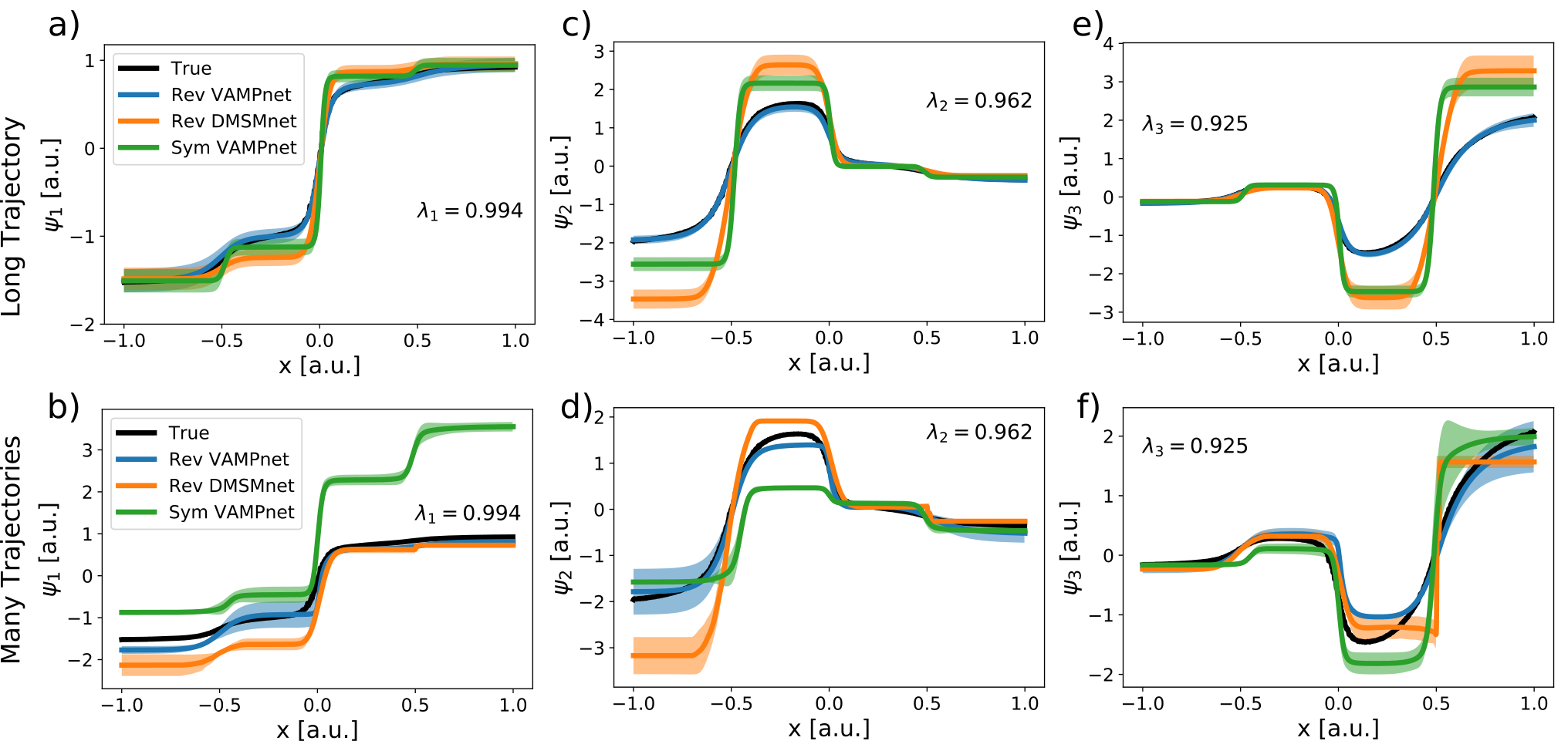
Finally, we compare the approximation quality of the three slowest non-trivial eigenfunctions for the Prinz potential for the three methods (Fig. 4). The data from the analysis before is reused of a single trajectory of length 50,000 frames, and of 10,000 trajectories 11 frames each. We compare the eigenfunctions against a numerical approximation of the true eigenfunctions by a transition matrix computed for a direct uniform 1,000-state discretization of the $x$ -axis for $2\cdot 10^{7}$ frames as before Prinz et al. 2011b.

The RevVAMPnet is approximating accurately the true eigenfunctions for all settings . In particular, it is able to recover the eigenfunctions remarkably even in the case of the biased data. The SymVAMPnet results are consistent with previous observations: the approximation of the first two eigenfunctions of the non-equilibrium data (Fig. 4b,d) are strongly biased, resulting in the underestimation of the implied timescales. The constraints in the case of the RevDMSM lead to less smoothly changing eigenfunctions and therefore less accurate approximations. In the case of the long trajectory, both the SymVAMPnet and the RevDMSM exhibit a stepwise behavior of the eigenfunctions, as they tend to result in a harder assignment of states $\boldsymbol{\chi}$ . Note that for SymVAMPnet this can be alleviated by avoiding a SoftMax clustering in the last layer and rather directly mapping onto the eigenfunctions Chen et al. 2019.

Refer to caption — Figure 4: Estimating the three slowest eigenfunction on the Prinz dataset with a RevVAMPnet, a SymVAMPnet, and a RevDMSM. a, c, e) Comparison of the eigenfunction estimated on one long trajectory. b, d, f) Comparison for many short trajectories having an off-equilibrium starting point distribution. Errors are estimated over 5 runs as two sigma intervals.

7 Conclusion

We have introduced an end-to-end deep learning framework for molecular kinetics that allows us to learn high-quality Markov models with physical constraints such as reversibility and non-negativity of the learned transition matrix. The proposed method is generally applicable for reversible/non-reversible Markov State and Koopman models depending on which constraints are enforced, thus it can be seen as an extension and generalization of previous models such as VAMPnets and DeepMSMs. Additionally, the optimization for the state classification and the reversible transition matrix are not explicitly separate processing steps compared to Chen et al. 2019. The proposed method is able to estimate dynamical and stationary properties even from highly biased data and gives state of the art results when studying the slow processes and stationary characteristics of a small toy model. We also proved that our model is a universal approximator of reversible Markov Processes and fulfills the reversibility property with respect to the estimated normalized stationary distribution.

Despite these advantages, a remaining concern is the optimization procedure, which requires a good balance when fitting the three trainable units at the same time. However, we are confident that the used protocol of first fixing $\boldsymbol{\chi}$ and resetting $\mathbf{u}$ to optimal values according to a non-reversible Koopman model during the training process establishes a reproduceable procedure.

Furthermore, we expect that the maximum likelihood formulation of the proposed method allows us to develop deep learning variants of multi-ensemble MSMs (Wu et al. 2016; Wu et al. 2014; Chodera et al. 2011; Prinz et al. 2011a; Rosta and Hummer 2015; Mey et al. 2014) that alleviate rare event sampling, and augmented MSMs Olsson et al. 2017 that incorporate experimental data into the model estimation.

8 Acknowledgements

This work was funded by the European Research Commission (ERC CoG “ScaleCell”), Deutsche Forschungsgemeinschaft (CRC 1114/A04, Transregio 186/A12, NO 825/4– 1, Dynlon P8), and the “1000-Talent Program of Young Scientists in China”. Part of this research was performed while the author was visiting the Institute for Pure and Applied Mathematics (IPAM), which is supported by the National Science Foundation (Grant No. DMS-1440415).

References

Bollt and Santitissadeekorn (2013) E. M. Bollt and N. Santitissadeekorn. Applied and Computational Measurable Dynamics. SIAM, 2013.
Boninsegna et al. (2015) L. Boninsegna, G. Gobbo, F. Noé, and C. Clementi. Investigating molecular kinetics by variationally optimized diffusion maps. J. Chem. Theory Comput., 11:5947–5960, 2015.
Bowman et al. (2009) G. R. Bowman, K. A. Beauchamp, G. Boxer, and V. S. Pande. Progress and challenges in the automated construction of Markov state models for full protein systems. J. Chem. Phys., 131:124101, 2009.
Bowman et al. (2014) G. R. Bowman, V. S. Pande, and F. Noé, editors. An Introduction to Markov State Models and Their Application to Long Timescale Molecular Simulation., volume 797 of Advances in Experimental Medicine and Biology. Springer Heidelberg, 2014.
Brunton et al. (2016) S. L. Brunton, J. L. Proctor, and J. N. Kutz. Discovering governing equations from data by sparse identification of nonlinear dynamical systems. Proceedings of the National Academy of Sciences, 113(15):3932–3937, 2016.
Buch et al. (2011) I. Buch, T. Giorgino, and G. De Fabritiis. Complete reconstruction of an enzyme-inhibitor binding process by molecular dynamics simulations. Proc. Natl. Acad. Sci. USA, 108:10184–10189, 2011. ISSN 1091-6490. 10.1073/pnas.1103547108.
Chen et al. (2019) W. Chen, H. Sidky, and A. L. Ferguson. Nonlinear discovery of slow molecular modes using state-free reversible vampnets. The Journal of Chemical Physics, 150(21):214114, Jun 2019. ISSN 1089-7690. 10.1063/1.5092521. URL http://dx.doi.org/10.1063/1.5092521.
Chodera and Noé (2014) J. D. Chodera and F Noé. Markov state models of biomolecular conformational dynamics. Curr. Opin. Struc. Biol., 25:135–144, 2014.
Chodera et al. (2007) J. D. Chodera, K. A. Dill, N. Singhal, V. S. Pande, W. C. Swope, and J. W. Pitera. Automatic discovery of metastable states for the construction of Markov models of macromolecular conformational dynamics. J. Chem. Phys., 126:155101, 2007.
Chodera et al. (2011) J. D. Chodera, W. C. Swope, F. Noé, J.-H. Prinz, and V. S. Pande. Dynamical reweighting: Improved estimates of dynamical properties from simulations at multiple temperatures. J. Phys. Chem., 134:244107, 2011.
Chollet et al. (2015) F. Chollet et al. Keras. https://github.com/fchollet/keras, 2015.
Dellnitz et al. (2001) M. Dellnitz, G. Froyland, and O. Junge. The algorithms behind gaio - set oriented numerical methods for dynamical systems. In Ergodic theory, analysis, and efficient simulation of dynamical systems, pages 145–174. Springer, 2001.
Doerr et al. (2016) S. Doerr, M. J. Harvey, F. Noé, and G. De Fabritiis. HTMD: High-Throughput Molecular Dynamics for Molecular Discovery. J. Chem. Theory Comput., 12:1845–1852, 2016.
et al. (2015) M. Abadi et al. TensorFlow: Large-scale machine learning on heterogeneous systems, 2015. URL http://tensorflow.org/. Software available from tensorflow.org.
Froyland et al. (2014) G. Froyland, G. A. Gottwald, and A. Hammerlindl. A computational method to extract macroscopic variables and their dynamics in multiscale systems. SIAM Journal on Applied Dynamical Systems, 13(4):1816–1846, 2014.
Froyland et al. (2016) G. Froyland, C. González-Tokman, and T. M. Watson. Optimal mixing enhancement by local perturbation. SIAM Review, 58(3):494–513, 2016.
Harmeling et al. (2003) S. Harmeling, A. Ziehe, M. Kawanabe, and K.-R. Müller. Kernel-based nonlinear blind source separation. Neur. Comp., 15:1089–1124, 2003.
Keller et al. (2010) B. G. Keller, X. Daura, and W. F. van Gunsteren. Comparing geometric and kinetic cluster algorithms for molecular simulation data. J. Chem. Phys., 132:074110, 2010. ISSN 1089-7690. 10.1063/1.3301140. URL http://dx.doi.org/10.1063/1.3301140.
Kingma and Ba (2014) D. P. Kingma and J. Ba. Adam: A method for stochastic optimization. CoRR, abs/1412.6980, 2014. URL http://arxiv.org/abs/1412.6980.
Kohlhoff et al. (2014) K. J. Kohlhoff, D. Shukla, M. Lawrenz, G. R. Bowman, D. E. Konerding, D. Belov, R. B. Altman, and V. S. Pande. Cloud-based simulations on google exacycle reveal ligand modulation of gpcr activation pathways. Nat. Chem., 6:15–21, 2014.
Konrad et al. (2001) A. Konrad, B. Y. Zhao, A. D. Joseph, and R. Ludwig. A markov-based channel model algorithm for wireless networks. In Proceedings of the 4th ACM international workshop on Modeling, analysis and simulation of wireless and mobile systems, pages 28–36. ACM, 2001.
Koopman (1931) B. O. Koopman. Hamiltonian systems and transformations in hilbert space. Proc. Natl. Acad. Sci. USA, 17:315–318, 1931.
Krivov and Karplus (2004) S. V. Krivov and M. Karplus. Hidden complexity of free energy surfaces for peptide (protein) folding. Proc. Nat. Acad. Sci. USA, 101:14766–14770, 2004.
Lindorff-Larsen et al. (2011) K. Lindorff-Larsen, S. Piana, R. O. Dror, and D. E. Shaw. How fast-folding proteins fold. Science, 334:517–520, 2011.
Ma et al. (2001) Y. Ma, J. J. Han, and K. S. Trivedi. Composite performance and availability analysis of wireless communication networks. IEEE Transactions on Vehicular Technology, 50(5):1216–1223, 2001.
Mardt et al. (2018) A. Mardt, L. Pasquali, H. Wu, and F. Noé. Vampnets: Deep learning of molecular kinetics. Nat. Commun., 9:5, 2018.
McGibbon and Pande (2015) R. T. McGibbon and V. S. Pande. Variational cross-validation of slow dynamical modes in molecular kinetics. J. Chem. Phys., 142:124105, 2015.
Metzner et al. (2009) P. Metzner, C. Schütte, and E. Vanden-Eijnden. Transition Path Theory for Markov Jump Processes. Multiscale Model. Simul., 7:1192–1219, 2009.
Mey et al. (2014) A. S. J. S. Mey, H. Wu, and F. Noé. xTRAM: Estimating equilibrium expectations from time-correlated simulation data at multiple thermodynamic states. Phys. Rev. X, 4:041018, 2014.
Mezić (2005) I. Mezić. Spectral properties of dynamical systems, model reduction and decompositions. Nonlinear Dynam., 41:309–325, 2005.
Mezić (2013) I. Mezić. Analysis of fluid flows via spectral properties of the koopman operator. Annual Review of Fluid Mechanics, 45:357–378, 2013.
Molgedey and Schuster (1994) L. Molgedey and H. G. Schuster. Separation of a mixture of independent signals using time delayed correlations. Phys. Rev. Lett., 72:3634–3637, 1994. 10.1103/PhysRevLett.72.3634.
Noé (2008) F. Noé. Probability Distributions of Molecular Observables computed from Markov Models. J. Chem. Phys., 128:244103, 2008.
Noé and Clementi (2015) F. Noé and C. Clementi. Kinetic distance and kinetic maps from molecular dynamics simulation. J. Chem. Theory Comput., 11:5002–5011, 2015.
Noé and Clementi (2017) F. Noé and C. Clementi. Collective variables for the study of long-time kinetics from molecular trajectories: theory and methods. Curr. Opin. Struc. Biol., 43:141–147, 2017.
Noé and Nüske (2013) F. Noé and F. Nüske. A variational approach to modeling slow processes in stochastic dynamical systems. Multiscale Model. Simul., 11:635–655, 2013.
Noé et al. (2007) F. Noé, I. Horenko, C. Schütte, and J. C. Smith. Hierarchical Analysis of Conformational Dynamics in Biomolecules: Transition Networks of Metastable States. J. Chem. Phys., 126:155102, 2007.
Noé et al. (2009) F. Noé, C. Schütte, E. Vanden-Eijnden, L. Reich, and T. R. Weikl. Constructing the full ensemble of folding pathways from short off-equilibrium simulations. Proc. Natl. Acad. Sci. USA, 106:19011–19016, 2009.
Noé et al. (2016) F. Noé, R. Banisch, and C. Clementi. Commute maps: separating slowly-mixing molecular configurations for kinetic modeling. J. Chem. Theory Comput., 12:5620–5630, 2016.
Nüske et al. (2014) F. Nüske, B. G. Keller, G. Pérez-Hernández, A. S. J. S. Mey, and F. Noé. Variational approach to molecular kinetics. J. Chem. Theory Comput., 10:1739–1752, 2014.
Nüske et al. (2016) F. Nüske, R. Schneider, F. Vitalini, and F. Noé. Variational tensor approach for approximating the rare-event kinetics of macromolecular systems. J. Chem. Phys., 144:054105, 2016.
Olsson et al. (2017) S. Olsson, H. Wu, F. Paul, C. Clementi, and F. Noé. Combining experimental and simulation data of molecular processes via augmented markov models. Proc. Natl. Acad. Sci. USA, 114:8265–8270, 2017.
Perez-Hernandez et al. (2013) G. Perez-Hernandez, F. Paul, T. Giorgino, G. D Fabritiis, and Frank Noé. Identification of slow molecular order parameters for markov model construction. J. Chem. Phys., 139:015102, 2013.
Plattner et al. (2017) N. Plattner, S. Doerr, G. De Fabritiis, and F. Noé. Protein-protein association and binding mechanism resolved in atomic detail. Nat. Chem., 9:1005–1011, 2017.
Prinz et al. (2011a) J.-H. Prinz, J. D. Chodera, V. S. Pande, W. C. Swope, J. C. Smith, and F. Noé. Optimal use of data in parallel tempering simulations for the construction of discrete-state markov models of biomolecular dynamics. J. Chem. Phys., 134:244108, 2011a.
Prinz et al. (2011b) J.-H. Prinz, H. Wu, M. Sarich, B. G. Keller, M. Senne, M. Held, J. D. Chodera, C. Schütte, and F. Noé. Markov models of molecular kinetics: Generation and validation. J. Chem. Phys., 134:174105, 2011b.
Reubold et al. (2015) T. F. Reubold, K. Faelber, N. Plattner, Y. Posor, K. Branz, U. Curth, J. Schlegel, R. Anand, D. Manstein, F. Noé, V. Haucke, O. Daumke, and S. Eschenburg. Crystal structure of the dynamin tetramer. Nature, 525:404–408, 2015.
Rosta and Hummer (2015) E. Rosta and G. Hummer. Free energies from dynamic weighted histogram analysis using unbiased markov state model. J. Chem. Theory Comput., 11:276–285, 2015.
Rowley et al. (2009) C. W. Rowley, I. Mezić, S. Bagheri, P. Schlatter, and D. S. Henningson. Spectral analysis of nonlinear flows. J. Fluid Mech., 641:115, nov 2009. 10.1017/s0022112009992059. URL http://dx.doi.org/10.1017/S0022112009992059.
Scherer et al. (2019) M. K. Scherer, B. E. Husic, M. Hoffmann, F. Paul, H. Wu, and F. Noé. Variational selection of features for molecular kinetics. The Journal of Chemical Physics, 150(19):194108, 2019. 10.1063/1.5083040. URL https://doi.org/10.1063/1.5083040.
Schmid (2010) P. J. Schmid. Dynamic mode decomposition of numerical and experimental data. J. Fluid Mech., 656:5–28, jul 2010. 10.1017/s0022112010001217. URL http://dx.doi.org/10.1017/S0022112010001217.
Schütte and Klus (2016) C. Schütte and S. Klus. Towards tensor-based methods for the numerical approximation of the perron–frobenius and koopman operator. Journal of Computational Dynamics, 3(2):139–161, Nov 2016. ISSN 2158-2491. 10.3934/jcd.2016007. URL http://dx.doi.org/10.3934/jcd.2016007.
Schütte et al. (1999) C. Schütte, A. Fischer, W. Huisinga, and P. Deuflhard. A Direct Approach to Conformational Dynamics based on Hybrid Monte Carlo. J. Comput. Phys., 151:146–168, 1999.
Schwantes and Pande (2013) C. R. Schwantes and V. S. Pande. Improvements in markov state model construction reveal many non-native interactions in the folding of ntl9. J. Chem. Theory Comput., 9:2000–2009, 2013.
Schwantes and Pande (2015) C. R. Schwantes and V. S. Pande. Modeling molecular kinetics with tica and the kernel trick. J. Chem. Theory Comput., 11:600–608, 2015.
Shukla et al. (2014) D. Shukla, Y. Meng, B. Roux, and V. S. Pande. Activation pathway of src kinase reveals intermediate states as targets for drug design. Nat. Commun., 5:3397, 2014.
Silva et al. (2014) Daniel-Adriano Silva, Dahlia R. Weiss, Fátima Pardo Avila, Lin-Tai Da, Michael Levitt, Dong Wang, and Xuhui Huanga. Millisecond dynamics of rna polymerase ii translocation at atomic resolution. Proc. Natl. Acad. Sci. USA, 111:7665–7670, 2014.
Song et al. (2013) L. Song, K. Fukumizu, and A. Gretton. Kernel embeddings of conditional distributions: A unified kernel framework for nonparametric inference in graphical models. IEEE Signal Processing Magazine, 30(4):98–111, 2013.
Swope et al. (2004) W. C. Swope, J. W. Pitera, and F. Suits. Describing protein folding kinetics by molecular dynamics simulations: 1. Theory. J. Phys. Chem. B, 108:6571–6581, 2004.
Trendelkamp-Schroer and Noé (2013) B. Trendelkamp-Schroer and F. Noé. Efficient bayesian estimation of markov model transition matrices with given stationary distribution. J. Phys. Chem., 138:164113., 2013.
Trendelkamp-Schroer et al. (2015) B. Trendelkamp-Schroer, H. Wu, F. Paul, and F. Noé. Estimation and uncertainty of reversible markov models. J. Chem. Phys., 143:174101, 2015.
Tu et al. (2014) J. H. Tu, C. W. Rowley, D. M. Luchtenburg, S. L. Brunton, and J. N. Kutz. On dynamic mode decomposition: Theory and applications. J. Comput. Dyn., 1(2):391–421, dec 2014. 10.3934/jcd.2014.1.391.
W. E and E. Vanden-Eijnden (2006) W. E and E. Vanden-Eijnden. Towards a Theory of Transition Paths. J. Stat. Phys., 123:503–523, 2006. ISSN 0022-4715. 10.1007/s10955-005-9003-9. URL http://dx.doi.org/10.1007/s10955-005-9003-9.
Williams et al. (2015) M. O. Williams, I. G. Kevrekidis, and C. W. Rowley. A data–driven approximation of the koopman operator: Extending dynamic mode decomposition. J. Nonlinear Sci., 25:1307–1346, 2015.
Wu and Noé (2015) H. Wu and F. Noé. Gaussian markov transition models of molecular kinetics. J. Chem. Phys., 142:084104, 2015.
Wu and Noé (2019) H. Wu and F Noé. Variational approach for learning markov processes from time series data. Journal of Nonlinear Science, Aug 2019. ISSN 1432-1467. 10.1007/s00332-019-09567-y. URL https://doi.org/10.1007/s00332-019-09567-y.
Wu et al. (2014) H. Wu, A. S. J. S. Mey, E. Rosta, and F. Noé. Statistically optimal analysis of state-discretized trajectory data from multiple thermodynamic states. J. Chem. Phys., 141:214106, 2014.
Wu et al. (2016) H. Wu, F. Paul, C. Wehmeyer, and F. Noé. Multiensemble markov models of molecular thermodynamics and kinetics. Proc. Natl. Acad. Sci. USA, 113(23):E3221–E3230, 2016. 10.1073/pnas.1525092113.
Wu et al. (2017) H. Wu, F. Nüske, F. Paul, S. Klus, P. Koltai, and F. Noé. Variational koopman models: slow collective variables and molecular kinetics from short off-equilibrium simulations. J. Chem. Phys., 146:154104, 2017.
Wu et al. (2018) H. Wu, A. Mardt, L. Pasquali, and F. Noe. Deep generative markov state models. In Advances in Neural Information Processing Systems, pages 3975–3984, 2018.
Xie et al. (2019) T. Xie, A. France-Lanord, Y. Wang, Y. Shao-Horn, and J. C. Grossman. Graph dynamical networks for unsupervised learning of atomic scale dynamics in materials. Nature communications, 10(1):2667, 2019.
Ziehe and Müller (1998) A. Ziehe and K.-R. Müller. TDSEP — an efficient algorithm for blind separation using time structure. In ICANN 98, pages 675–680. Springer Science and Business Media, 1998. 10.1007/978-1-4471-1599-1_103.

9 Appendix

9.1 Proof of normalization

We show that the dynamical model (5) has a normalized transition and equilibrium density. By defining

\mu(\mathbf{x})=\mathbf{u}^{T}\boldsymbol{\chi}(\mathbf{x})\rho_{1}(\mathbf{x}),

we can obtain that

	$\displaystyle\int p_{\tau}(\mathbf{x},\mathbf{y})\mathrm{d}\mathbf{y}$	$\displaystyle=\int\boldsymbol{\chi}(\mathbf{x})^{T}\mathbf{S}\boldsymbol{\chi}(\mathbf{y})\boldsymbol{\chi}(\mathbf{y})^{T}\mathbf{u}\rho_{1}(\mathbf{y})\mathrm{d}\mathbf{y}$
		$\displaystyle=\boldsymbol{\chi}(\mathbf{x})^{T}\mathbf{S}\mathbf{C}_{\tau\tau}^{\prime}\mathbf{u}=1$
	$\displaystyle\int\mu(\mathbf{x})\mathrm{d}\mathbf{x}$	$\displaystyle=\mathbf{u}^{T}\bar{\boldsymbol{\chi}}=1$

9.2 Proof of proposition 1

Proof. Since $\{\mathbf{x}_{t}\}$ is reversible, its transition density can be decomposed as

p_{\tau}(\mathbf{x},\mathbf{y})=\sum_{i=1}^{\infty}\lambda_{i}\varphi_{i}(\mathbf{x})\varphi_{i}(\mathbf{y})\mu(\mathbf{y}),

where $\varphi_{i}$ is the eigenfunction corresponding to the eigenvalue $\lambda_{i},$ $\{\varphi_{1},\varphi_{2},...\}$ is an orthonormal basis of the Hilbert space $\{f|\langle f,f\rangle_{\mu}<\infty\}$ defined by the inner product

\langle f,g\rangle_{\mu}=\int f(\mathbf{x})g(\mathbf{x})\mu(\mathbf{x})\mathrm{d\mathbf{x}},

and $(\lambda_{1},\varphi_{1})=(1,\mu)$ .

Considering a (d+1)-dimensional model

	$\displaystyle\boldsymbol{\chi}(\mathbf{x})^{T}$	$\displaystyle=(\boldsymbol{\varphi}(\mathbf{x})^{T},w_{1}(\mathbf{x})),$
	$\displaystyle\mathbb{\mathbf{S}}$	$\displaystyle=\left[\begin{array}[]{cc}\mathbb{\boldsymbol{\Lambda}}\\ &0\end{array}\right],$
	$\displaystyle\mathbf{\mathbf{u}}$	$\displaystyle=(0,...,0,1)^{T},$

we can obtain its transition density as

	$\displaystyle\hat{p}_{\tau}(\mathbf{x},\mathbf{y})$	$\displaystyle=\boldsymbol{\chi}(\mathbf{x})^{T}\mathbf{S}\boldsymbol{\chi}(\mathbf{y})\rho_{1}(\mathbf{y})\boldsymbol{\chi}(\mathbf{y})^{T}\mathbf{u}$
		$\displaystyle=\boldsymbol{\varphi}(\mathbf{x})^{T}\boldsymbol{\Lambda}\boldsymbol{\varphi}(\mathbf{y})\mu(\mathbf{y}),$

where $\boldsymbol{\varphi}=(\varphi_{1},...,\varphi_{d})^{T},$ $\boldsymbol{\Lambda}=\mathrm{diag}(\lambda_{1},...,\lambda_{d})$ and $w_{1}(\mathbf{x})=\rho_{1}(\mathbf{x})^{-1}\mu(\mathbf{x})$ .

Then the Koopman operator $\mathcal{\hat{K_{\tau}}}$ deduced from this model satisfies

	$\displaystyle\|\|\mathcal{\hat{K_{\tau}^{*}}-\mathcal{K_{\tau}}\|\|_{\mathrm{HS}}^{\mathrm{2}}}$	$\displaystyle=\int\int\rho_{0}(\mathbf{x})\frac{(\hat{p}_{\tau}(\mathbf{x},\mathbf{y})-p_{\tau}(\mathbf{x},\mathbf{y}))^{2}}{\rho_{1}(\mathbf{y})}\mathrm{d\mathbf{x}d\mathbf{y}}$
		$\displaystyle=\int\int\rho_{0}(\mathbf{x})\left(\sum_{i=d+1}^{\infty}\lambda_{i}\varphi_{i}(\mathbf{x})\varphi_{i}(\mathbf{y})\right)^{2}w_{1}(\mathbf{y})\mu(\mathbf{y})\mathrm{d\mathbf{x}d\mathbf{y}}$
		$\displaystyle\leq C_{1}\int\rho_{0}(\mathbf{x})\sum_{i=d+1}^{\infty}\lambda_{i}^{2}\varphi_{i}(\mathbf{x})^{2}\mathrm{d\mathbf{x}}$
		$\displaystyle\leq C_{0}C_{1}\int\mu(\mathbf{x})\sum_{i=d+1}^{\infty}\lambda_{i}^{2}\varphi_{i}(\mathbf{x})^{2}\mathrm{d\mathbf{x}}$
		$\displaystyle=C_{0}C_{1}\sum_{i=d+1}^{\infty}\lambda_{i}^{2},$

and the approximation error of the optimal (d+1)-dimensional model is also bounded by $C_{0}C_{1}\sum_{i=d+1}^{\infty}\lambda_{i}^{2}.$

9.3 Proof of proposition 2

Proof. Since $\{\mathbf{x}_{t}\}$ is reversible, $\mathcal{K_{\tau}}$ can be decomposed as

\mathcal{K_{\tau}}f=\sum_{i=1}^{\infty}\lambda_{i}\langle f,\varphi_{i}\rangle_{\mu}\varphi_{i}

with $\lambda_{1}=1$ and $\varphi_{1}\equiv 1$ . According to the VAMP theory and considering that the proposed model is a specific case of

\hat{p}_{\tau}(\mathbf{x},\mathbf{y})=\boldsymbol{\chi}(\mathbf{x})^{T}\mathbf{S}\boldsymbol{\chi}(\mathbf{y})\mu(\mathbf{y}),

Eq. 12 can be proven.

If $\boldsymbol{\varphi}=(\varphi_{1},...,\varphi_{d})^{T}$ can be represented by linear combinations of $\boldsymbol{\chi}(\mathbf{x})$ , i.e., there is an invertible matrix $\mathbf{R}=[R_{ij}]\in\mathbb{R}^{d\times d}$ so that

\boldsymbol{\varphi}=\mathbf{R}\boldsymbol{\chi}.

We can then construct the following model

	$\displaystyle\hat{p}_{\tau}(\mathbf{x},\mathbf{y})$	$\displaystyle=\boldsymbol{\chi}(\mathbf{x})^{T}\mathbf{S}\boldsymbol{\chi}(\mathbf{y})\boldsymbol{\chi}(\mathbf{y})^{T}\mathbf{u}\mu(\mathbf{y})$
		$\displaystyle=\boldsymbol{\varphi}(\mathbf{x})^{T}\mathbf{R}^{-T}\mathbf{SR}^{-1}\boldsymbol{\varphi}(\mathbf{y})\boldsymbol{\varphi}(\mathbf{y})^{T}\mathbf{R}^{-T}\mathbf{u}\mu(\mathbf{y})$
		$\displaystyle=\boldsymbol{\varphi}(\mathbf{x})^{T}\boldsymbol{\Lambda}\boldsymbol{\varphi}(\mathbf{y})\mu(\mathbf{y}),$

where

	$\displaystyle\mathbf{S}$	$\displaystyle=\mathbf{R}^{T}\boldsymbol{\Lambda}\mathbf{R},$
	$\displaystyle\mathbf{u}$	$\displaystyle=\mathbf{R}^{T}(1,0,....,0)^{T},$

and $\boldsymbol{\Lambda}=\mathrm{diag}(\lambda_{1},...,\lambda_{d})$ . It can be verified that the VAMP-E score of this model is equal to $\sum_{i=1}^{d}\lambda_{i}^{2}$ .

9.4 Relationships to traditional Markov State Models

Since in traditional MSMs the state definition $\boldsymbol{\chi}$ usually consists of a set of indicator functions partitioning the full state space into Markov States, we show how in that case, for the right choices of $\mathbf{u}$ and $\mathbf{S}$ , our model obtains the expected stationary and transition distribution.

Let $\boldsymbol{\chi}$ be the indicator functions of Markov states, $\boldsymbol{\pi}$ be the stationary distribution vector, $\boldsymbol{\pi}_{\rho}=\bar{\boldsymbol{\chi}}$ the empirical distribution vector of states, and

	$\displaystyle\mathbf{u}$	$\displaystyle=\boldsymbol{\Pi}_{\rho}^{-1}\boldsymbol{\pi},$
	$\displaystyle\mathbf{S}$	$\displaystyle=\mathbf{P}\boldsymbol{\Pi}^{-1},$

where $\boldsymbol{\Pi}=\mathrm{diag}(\boldsymbol{\pi}),$ $\boldsymbol{\Pi}_{\rho}=\mathrm{diag}(\boldsymbol{\pi}_{\rho})$ , and $\mathbf{P}$ is the transition matrix. We can then express $\mu(\mathbf{x})$ as:

	$\displaystyle\mu(\mathbf{x})$	$\displaystyle=\mathbf{u}^{T}\boldsymbol{\chi}(\mathbf{x})\rho(\mathbf{x})$
		$\displaystyle=\boldsymbol{\pi}^{T}\boldsymbol{\Pi}_{\rho}^{-1}\boldsymbol{\chi}(\mathbf{x})\rho(\mathbf{x}),$

and

	$\displaystyle p_{\tau}(\mathbf{x},\mathbf{y})$	$\displaystyle=\boldsymbol{\chi}(\mathbf{x})^{T}\mathbf{P}\boldsymbol{\Pi}^{-1}\boldsymbol{\chi}(\mathbf{y})\rho(\mathbf{y})\boldsymbol{\chi}(\mathbf{y})^{T}\boldsymbol{\Pi}_{\rho}^{-1}\boldsymbol{\pi}$
		$\displaystyle=\boldsymbol{\chi}(\mathbf{x})^{T}\mathbf{P}\boldsymbol{\Pi}_{\rho}^{-1}\boldsymbol{\chi}(\mathbf{y})\rho(\mathbf{y})\boldsymbol{\chi}(\mathbf{y})^{T}\boldsymbol{\Pi}^{-1}\boldsymbol{\pi}$
		$\displaystyle=\boldsymbol{\chi}(\mathbf{x})^{T}\mathbf{P}\boldsymbol{\Pi}_{\rho}^{-1}\boldsymbol{\chi}(\mathbf{y})\rho(\mathbf{y}).$