MISCONFIGURATION MANAGEMENT
OF NETWORK SECURITY COMPONENTS

Frédéric Cuppens Nora Cuppens-Boulahia Affiliation: GET/ENST-Bretagne,2, rue de la Châtaigneraie,35576 Cesson Sévigné - France{frederic.cuppens,nora.cuppens}@enst-bretagne.fr Affiliation: GET/ENST-Bretagne,2, rue de la Châtaigneraie,35576 Cesson Sévigné - France{frederic.cuppens,nora.cuppens}@enst-bretagne.fr Joaquín García-Alfaro Affiliation: GET/ENST-Bretagne,2, rue de la Châtaigneraie,35576 Cesson Sévigné - France{frederic.cuppens,nora.cuppens}@enst-bretagne.fr Affiliation: dEIC/UAB,Edifici Q, Campus de Bellaterra,08193, Bellaterra, Barcelona - Spainjoaquin.garcia@uab.es

Abstract

Many companies and organizations use firewalls to control the access to their network infrastructure. Firewalls are network security components which provide means to filter traffic within corporate networks, as well as to police incoming and outcoming interaction with the Internet. For this purpose, it is necessary to configure firewalls with a set of filtering rules. Nevertheless, the existence of errors in a set of filtering rules is very likely to degrade the network security policy. The discovering and removal of these configuration errors is a serious and complex problem to solve. In this paper, we present a set of algorithms for such a management. Our approach is based on the analysis of relationships between the set of filtering rules. Then, a subsequent rewriting of rules will derive from an initial firewall setup – potentially misconfigured – to an equivalent one completely free of errors. At the same time, the algorithms will detect useless rules in the initial firewall configuration.

1 Introduction

order			condition			decision
	(p)rotocol	(s)ource	(sP)ort	(d)estination	(dP)ort
1	any	xxx.xxx.xxx.[001,030]	any	xxx.xxx.xxx.[020,045]	any	deny
2	any	xxx.xxx.xxx.[020,060]	any	xxx.xxx.xxx.[025,035]	any	accept
3	any	xxx.xxx.xxx.[040,070]	any	xxx.xxx.xxx.[020,045]	any	accept
4	any	xxx.xxx.xxx.[015,045]	any	xxx.xxx.xxx.[025,030]	any	deny
5	any	xxx.xxx.xxx.[025,045]	any	xxx.xxx.xxx.[020,040]	any	accept

Table 1: Example of a set of filtering rules with five condition attributes.

The use of firewalls is the dominant method for companies and organizations to segment access control within their own networks. They are typically deployed to filter traffic between trusted and untrusted zones of corporate networks, as well as to police their incoming and outcoming interaction with the Internet¹¹ 1 Firewalls also implement other functionalities, such as Proxying and Network Address Transfer (NAT), but it is not the purpose of this paper to cover these functionalities..

Firewalls are network security components, with several interfaces associated with the different zones of the network. A company may partition, for instance, its network into three different zones: a demilitarized zone (DMZ for short), a private network and a zone for security administration. In this case, one may use a firewall with three interfaces associated with these three zones, as well as a fourth interface to control the access to the Internet.

In order to apply the filtering process, it is necessary to configure the firewall with a set of filtering rules (e.g., the set of filtering rules shown in Table 1). Each filtering rule typically specifies a $decision$ (e.g., $accept$ or $deny$ ) that applies to a set of $condition$ attributes, such as protocol, source, destination, and so on.

For our work, we define a filtering rule as follows:

R_{i}:\{condition_{i}\}\rightarrow decision_{i}

(1)

where $i$ is the relative position of the rule within the set of rules, $decision_{i}$ is a boolean expression in $\{accept,deny\}$ ²² 2 The $decision$ field may also be a combination of both $accept$ and $deny$ together with some other options such as a logging or jump options. For reasons of clarity we assume that just accept and deny are proper values., and $\{condition_{i}\}$ is a conjunctive set of condition attributes such that $\{condition_{i}\}$ equals $A_{1}\wedge A_{2}\wedge...\wedge A_{p}$ , and $p$ is the number of condition attributes of the given filtering rules.

The following example³³ 3 To simplify the example, the number of condition attributes, i.e., $p$ , is just two: (s)ource and (d)destination. We do not show the condition attributes (p)rotocol, (sP)ort, and (dP)ort, because their value will always be $true$ . shows the filtering rules of Table 1 using such a formalism.

$R_{1}:(s\in[1,30]\land d\in[20,45])\rightarrow deny$

$R_{2}:(s\in[20,60]\land d\in[25,35])\rightarrow accept$

$R_{3}:(s\in[40,70]\land d\in[20,45])\rightarrow accept$

$R_{4}:(s\in[15,45]\land d\in[25,30])\rightarrow deny$

$R_{5}:(s\in[25,45]\land d\in[20,40])\rightarrow accept$

When processing packages, conflicts due to rule overlaps can occur within the filtering policy. For instance, we can see in Figure 1 a geometrical representation of the main overlaps within the filtering rules of Table 1.

Figure 1: Main overlaps within the rules of Table 1

To solve these conflicts, most firewall implementations use a first matching strategy through the ordering of rules – such as the order field shown in Table 1. This way, each packet processed by the firewall is mapped to the decision of the rule with highest priority. This strategy introduces, however, new configuration errors, such as shadowing of rules and redundancy. For our work, we define these two general cases of firewall misconfiguration as follows.

Definition 1.1

Let $R$ be a set of filtering rules. Then $R$ has shadowing if and only if there exists at least one filtering rule, $R_{i}$ in $R$ , which never applies because all the packets that $R_{i}$ may match, are previously matched by another rule, or combination of rules, with higher priority in order.

Definition 1.2

Let $R$ be a set of filtering rules. Then $R$ has redundancy if and only if there exists at least one filtering rule, $R_{i}$ in $R$ , such that the following conditions hold: (1) $R_{i}$ is not shadowed by any other rule; (2) when removing $R_{i}$ from $R$ , the filtering result, i.e., the security policy, does not change.

The discovering and removal of both redundancy and shadowing is a serious problem which must be solved since a misconfigured set of filtering rules, if not handled correctly, is very likely to cause packets to be subject to the wrong actions, and to lead to a weak security policy.

In this paper, we present a set of algorithms for the discovering and removal of both redundancy and shadowing of rules. Our main objective is the following. Given a specific firewall setup, we want to analyze the existing firewall configuration to check whether there is errors in such a configuration, i.e., the set of filtering rules presents shadowing or redundancy as defined above.

Our approach is based on the relationships between the filtering rules’ parameters: coincidence, disjunction and inclusion. We use a rule transformation process that derive from a set of filtering rules to an equivalent and valid one that is completely free of both shadowing and redundancy.

The advantages of our proposal are threefold. First of all, after rewriting the rules one can verify that there is no redundancy nor shadowing in the resulting firewall configuration. Each redundant or shadowed rule – considered as useless during the audit process – will be removed from the initial set of filtering rules.

On the second hand, when such a detection occurs the discovering process will provide an evidence of error to the administration console. This way, the security officer in charge of the network can check from the initial specification, in order to verify the correctness of the whole process.

On the third hand, the resulting rules are completely disjoint, i.e., the ordering of rules is no longer relevant. Hence, one can perform a second transformation in a positive or negative manner: positive, when generating only permissions; and negative, when generating only prohibitions. Positive rewriting can be used in a closed policy whereas negative rewriting can be used in case of an open policy.

After performing this second rewriting, the security officer will have a clear view of the accepted traffic (in the case of positive rewriting) or the rejected traffic (in the case of negative rewriting).

The rest of this paper is organized as follows: Section 2 starts with an analysis of some related work. Then, Section 3 presents our algorithms and introduces some examples to validate the correctness of our approach. Section 4 analyzes the complexity of our proposed algorithms and overviews a performance study. Section 5 closes the paper with some conclusions and gives an outlook on future work.

2 Related Work

A first approach to get a firewall configuration free of errors is by applying a formal security model to express the network security policy. In [5], for example, a formal model is presented with this purpose. This way, a set of filtering rules, whose syntax is specific to a given firewall, may be generated using a transformation language. Nonetheless, this approach is not enough to ensure that the firewall configuration is completely free of errors.

Some other proposals, such as [1, 7, 2, 8, 3], provide means to directly manage misconfiguration. For instance, the authors in [1] consider that, in a configuration set, two rules are in conflict when the first rule in order matches some packets that match the second rule, and the second rule also matches some of the packets that match the first rule.

This approach is very limited since it does not detect what we consider serious misconfiguration errors, i.e., redundancy and shadowing of rules (cf. Section1, Def. 1.1 and Def. 1.2). What they detect is just a particular case of wrongly defined rules which cause ambiguity in the firewall configuration, and that is more efficiently defined as a combination of both redundancy and shadowing.

In [7], two new cases of misconfiguration are considered. First, a rule $R_{j}$ is defined as backward redundant if and only if there exists another rule $R_{i}$ with higher priority in order such that all the packets that match rule $R_{j}$ also match rule $R_{i}$ . On the other hand, a rule $R_{i}$ is defined as forward redundant if and only if there exists another rule $R_{j}$ with the same decision and less priority in order such that the following conditions hold: (1) all the packets that match $R_{i}$ also match $R_{j}$ ; (2) for each rule $R_{k}$ between $R_{i}$ and $R_{j}$ , and that matches all the packets that also match rule $R_{i}$ , $R_{k}$ has the same decision as $R_{i}$ .

Although this approach seems to head in the right direction, we consider our definitions (cf. Section1, Def. 1.1 and Def. 1.2) simpler and more general, because all possible backward and forward redundant rules are specific cases of both redundancy and shadowing, but not vice versa. For instance, given the following set of rules:

$R_{1}:s\in[10,50]\rightarrow deny$

$R_{2}:s\in[40,70]\rightarrow accept$

$R_{3}:s\in[50,80]\rightarrow accept$

Since rule $R_{2}$ comes after rule $R_{1}$ , rule $R_{2}$ only applies over the interval $[51,70]$ – i.e., $R_{2}$ is redundant with respect to rule $R_{3}$ . Their detection proposal, as defined above, cannot detect the redundancy of rule $R_{2}$ . Therefore, we point out this work as incomplete.

To our best knowledge, the authors of the firewall policy advisor [2, 3] propose the most efficient set of techniques and algorithms to detect redundancy and shadowing in different firewall configuration setups. In addition to the discovery process, their approach also attempts an optimal insertion of arbitrary rules into an existing configuration, through a tree based representation of the filtering criteria.

Nonetheless, and even though the efficiency of their proposed discovering algorithms and techniques is very promising, we also consider this approach as incomplete.

On the one hand, their approach is too weak since, given a misconfigured firewall, their discovering algorithms could not detect all the possible errors. For example, given the following set of rules:

$R_{1}:s\in[10,50]\rightarrow accept$

$R_{2}:s\in[40,90]\rightarrow accept$

$R_{3}:s\in[30,80]\rightarrow deny$

their approach cannot detect the shadowing over rule $R_{3}$ due to the union of rules $R_{1}$ and $R_{2}$ .

On the other hand, the authors do not cover, intentionally, an automatic rewriting of rules to correct the discovered errors. This way, it is the security officer who should perform the final changes.

Summing up, we believe that none of the identified related work provides a complete discovering of both redundancy and shadowing of rules – which are the cases we consider serious errors within firewalls configurations – as well as a proper handling of such a misconfiguration.

3 Proposed Algorithms

3.1 Detection Process

As pointed out in Section 1, our main objective is the discovering of both shadowing and redundancy errors inside an initial set of filtering rules $R$ . Such a detection process is a way to alert the security officer in charge of the network about these configuration errors, as well as to remove all the useless rules in the initial firewall configuration.

The data to be used for the detection process is the following. A set of rules $R$ as a dynamic linked-list⁴⁴ 4 A dynamic linked-list is a pointer-based data structure that can be used to properly represent the abstract notion of a dynamic list. of initial size $n$ , where $n$ equals $count(R)$ , and where each element is an associative array⁵⁵ 5 Associative arrays – also known as a map, lookup table, or dictionary – have strings as keys and behave more like two-column tables, where the first column is the key to access the value of the second column. with the strings $condition$ , $decision$ , $shadowing$ , and $redundancy$ as keys to access each necessary value.

To simplify, we assume one can access a linked-list through the operator $R_{i}$ , where $i$ is the relative position regarding the initial list size – $count(R)$ . We also assume one can add new values to the list as any other normal variable does ( $element\leftarrow value$ ), as well as to remove elements through the addition of an empty set ( $element\leftarrow\emptyset$ ). The internal order of elements from the linked-list $R$ keeps with the relative ordering of rules.

In turn, each element $R_{i}[condition]$ is an indexed array⁶⁶ 6 For our algorithms, we assume that the keys of an indexed array are integers, beginning at 1, and where one can identify the elements by their position. of size $p$ containing the set of conditions of each rule; each element $R_{i}[decision]$ is a boolean variable whose values are in $\{accept,deny\}$ ; each element $R_{i}[shadowing]$ is a boolean variable in $\{true,false\}$ ; each element $R_{i}[redundancy]$ is another boolean variable in $\{true,false\}$ . Both shadowing and redundancy variables of each rule are initialized to $false$ by default.

For reasons of clarity, we split the whole detection process and the removal of misconfiguration in two different processes. Thus, we define a main detection function (Algorithm 1), whose input is the initial set of filtering rules, $R$ , and an auxiliary function (Algorithm 2) whose input is two rules, $A$ and $B$ . Once executed, this auxiliary function returns a further rule, $C$ , whose set of condition attributes is the exclusion of the set of conditions from $A$ over $B$ . In order to simplify the representation of this second algorithm (cf. Algorithm 2), we use the notation $A_{i}$ as an abbreviation of the variable $A[condition][i]$ , an the notation $B_{i}$ as an abbreviation of the variable $B[condition][i]$ – where $i$ in $[1,p]$ .

We recall that the output of the main detection function is the set which results as a transformation of the initial set $R$ . This new set is equivalent to the initial one, $R$ , and all its rules are completely disjoint. Therefore, the resulting set is free of both redundancy and shadowing of rules, as well as any other possible configuration error.

begin

for $i\leftarrow 1$ to $(count(R)-1)$
do

for $j\leftarrow(i+1)$ to $count(R)$
do

R_{j}\leftarrow

exclusion (

R_{j}

R_{i}

); if $R_{j}[condition]=\emptyset$
then

R_{j}[shadowing]\leftarrow true

; end

end

Algorithm 1 detection(

R

)

begin

C[condition]\leftarrow\emptyset

;

C[decision]\leftarrow B[decision]

;

C[shadowing]\leftarrow false

;

C[redundancy]\leftarrow false

; forall the elements of $A[condition]$ and $B[condition]$ do

if $((A_{1}\cap B_{1})\neq\emptyset$ and
$(A_{2}\cap B_{2})\neq\emptyset$ and …
… and $(A_{p}\cap B_{p})\neq\emptyset)$
then

C[condition]\leftarrow C[condition]~\cup

{

(B_{1}-A_{1})\wedge B_{2}\wedge...\wedge B_{p}

(A_{1}\cap B_{1})\wedge(B_{2}-A_{2})\wedge...\wedge B_{p}

(A_{1}\cap B_{1})\wedge(A_{2}\cap B_{2})\wedge(B_{3}-A_{3})\wedge...\wedge B_{p}

...

(A_{1}\cap B_{1})\wedge...\wedge(A_{p-1}\cap B_{p-1})\wedge(B_{p}-A_{p})\}

;
else

C[condition]\leftarrow

(C[condition]\cup B[condition]

); end

end

return $C$ ; end

Algorithm 2 exclusion(

B

A

)

3.1.1 Applying the Algorithms

This section gives a short outlook on applying algorithms 1 and 2 over some representative examples.

Let us start applying the function exclusion (Algorithm 2) over a set of two rules $R_{i}$ and $R_{j}$ , each one of them with two condition attributes – (s)ource and (d)estination – and where rule $R_{j}$ has less priority in order than rule $R_{i}$ . In this first example:

$R_{i}[condition]=(s\in[80,100])\wedge(d\in[1,50])$

$R_{j}[condition]=(s\in[1,50])\wedge(d\in[1,50])$

since $(s\in[1,50])\cap(s\in[80,100])$ equals $\emptyset$ , the condition attributes of rules $R_{i}$ and $R_{j}$ are completely independent. Thus, the applying of $exclusion(R_{j},R_{i})$ is equal to $R_{j}[condition]$ .

The following three examples show the same execution over a set of condition attributes with different cases of conflict. A first case is the following:

$R_{i}[condition]=(s\in[1,60])\wedge(d\in[1,30])$

$R_{j}[condition]=(s\in[1,50])\wedge(d\in[1,50])$

where there is a main overlap of attribute $s$ from $R_{i}[condition]$ which completely excludes the same attribute on $R_{j}[condition]$ . Then, there is a second overlap of attribute $d$ from $R_{i}[condition]$ which partially excludes the range $[1,30]$ into attribute $d$ of $R_{j}[condition]$ , which becomes $d$ in $[31,50]$ . This way, $exclusion(R_{j},R_{i})\leftarrow\{(s\in[1,50])\wedge(d\in[31,50])\}$ ⁷⁷ 7 For reasons of clarity, we do not show the first empty set corresponding to the first overlap. If shown, the result should become as follows: $exclusion(R_{j},R_{i})\leftarrow\{\emptyset,(s\in[1,50])\wedge(d\in[31,50])\}$ .. In this other example:

$R_{i}[condition]=(s\in[1,60])\wedge(d\in[20,30])$

$R_{j}[condition]=(s\in[1,50])\wedge(d\in[1,50])$

there is two simple overlaps of both attributes $s$ and $d$ from $R_{i}[condition]$ to $R_{j}[condition]$ , such that $exclusion(R_{j},R_{i})$ becomes $\{(s\in[1,50])\wedge(d\in[1,19]),(s\in[1,50])\wedge(d\in[31,50])\}$ .

A more complete example is the following,

$R_{i}[condition]=(s\in[10,40])\wedge(d\in[20,30])$

$R_{j}[condition]=(s\in[1,50])\wedge(d\in[1,50])$

where $exclusion(R_{j},R_{i})$ becomes $\{(s\in[1,9])\wedge(d\in[1,50]),(s\in[41,50])\wedge(d\in[1,50]),(s\in[10,40])\wedge(d\in[1,19]),(s\in[10,40])\wedge(d\in[31,50])\}$ .

Regarding a full exclusion, let us show the following example,

$R_{i}[condition]=(s\in[1,60])\wedge(d\in[1,60])$

$R_{j}[condition]=(s\in[1,50])\wedge(d\in[1,50])$

where the set of condition attributes of rule $R_{i}$ completely excludes the ones of rule $R_{j}$ . Then, the applying of $exclusion(R_{j},R_{i})$ becomes an empty set (i.e., $\{\emptyset,\emptyset\}=\emptyset$ ). Hence, on a further execution of Algorithm 1 the shadowing field of rule $R_{j}$ (initialized as $false$ by default) would become $true$ (i.e., $R_{j}[shadowing]\leftarrow true$ ).

To conclude this section, let us show a complete execution of algorithms 1 and 2 over a set of filtering rules based on Table 1 – whose main overlaps have been previously shown in Figure 1.

$/*motivation~example*/$ $R_{1}:(s\in[1,30]\land d\in[20,45])\rightarrow deny$ $R_{2}:(s\in[20,60]\land d\in[25,35])\rightarrow accept$ $R_{3}:(s\in[40,70]\land d\in[20,45])\rightarrow accept$ $R_{4}:(s\in[15,45]\land d\in[25,30])\rightarrow deny$ $R_{5}:(s\in[25,45]\land d\in[20,40])\rightarrow accept$ $/*step~1*/$ $R_{1}:(s\in[1,30]\land d\in[20,45])\rightarrow deny$ $R_{2}:(s\in[31,60]\land d\in[25,35])\rightarrow accept$ $R_{3}:(s\in[40,70]\land d\in[20,45])\rightarrow accept$ $R_{4}:(s\in[31,45]\land d\in[25,30])\rightarrow deny$ $R_{5}:(s\in[31,45]\land d\in[20,40])\rightarrow accept$ $/*step~2*/$ $R_{1}:(s\in[1,30]\land d\in[20,45])\rightarrow deny$ $R_{2}:(s\in[31,60]\land d\in[25,35])\rightarrow accept$ $R_{3}:\{(s\in[61,70]\land d\in[20,45]),\\ ~~~~~~~~~(s\in[40,60]\land d\in[20,24]),\\ ~~~~~~~~~(s\in[40,60]\land d\in[36,45])\}\rightarrow accept$ $R_{4}:\emptyset\rightarrow deny$ $R_{5}:\{(s\in[31,45]\land d\in[20,24]),\\ ~~~~~~~~~(s\in[31,45]\land d\in[36,40])\}\rightarrow accept$ $/*step~3=step~4=resulting~rules*/$ $R_{1}:(s\in[1,30]\land d\in[20,45])\rightarrow deny$ $R_{2}:(s\in[31,60]\land d\in[25,35])\rightarrow accept$ $R_{3}:\{(s\in[61,70]\land d\in[20,45]),\\ ~~~~~~~~~(s\in[40,60]\land d\in[20,24]),\\ ~~~~~~~~~(s\in[40,60]\land d\in[36,45])\}\rightarrow accept$ $R_{5}:\{(s\in[31,39]\land d\in[20,24]),\\ ~~~~~~~~~(s\in[31,39]\land d\in[36,40])\}\rightarrow accept$ $/*warnings*/$ $R_{4}[shadowing]=true$

3.2 Correctness of the Algorithms

Definition 3.1

Let $R$ be a set of filtering rules and let $Tr(R)$ be the resulting filtering rules obtained by applying Algorithm 1 to $R$ .

Lemma 3.2

Let $R_{i}:condition_{i}\rightarrow decision_{i}$ and $R_{j}:condition_{j}\rightarrow decision_{j}$ be two filtering rules. Then $\{R_{i},R_{j}\}$ is equivalent to $\{R_{i},R^{\prime}_{j}\}$ where $R^{\prime}_{j}\leftarrow exclusion(R_{j},R_{i})$ .⁸⁸ 8 A set of proofs to validate the theorems and lemmas of this section is provided in [6].

Theorem 3.3

Let $R$ be a set of filtering rules and let $Tr(R)$ be the resulting filtering rules obtained by applying Algorithm 1 to $R$ . Then $R$ and $Tr(R)$ are equivalent.

Lemma 3.4

Let $R_{i}:condition_{i}\rightarrow decision_{i}$ and $R_{j}:condition_{j}\rightarrow decision_{j}$ be two filtering rules. Then rules $R_{i}$ and $R^{\prime}_{j}$ , where $R^{\prime}_{j}\leftarrow exclusion(R_{j},R_{i})$ will never simultaneously apply to any given packet.

Theorem 3.5

Let $R$ be a set of filtering rules and let $Tr(R)$ be the resulting filtering rules obtained by applying Algorithm 1 to $R$ . Then ordering the rules in $Tr(R)$ is no longer relevant.

Theorem 3.6

Let $R$ be a set of filtering rules and let $Tr(R)$ be the resulting filtering rules obtained by applying Algorithm 1 to $R$ . Then $Tr(R)$ is free from both shadowing and redundancy.

3.3 Complete Detection

Up to now, the result of Algorithm 1 offers a set of filtering rules, $Tr(R)$ , equivalent to an initial set of rules $R$ , and completely free of any possible relation between its rules. Nevertheless, there is a limitation on such an algorithm regarding the reporting of redundancy – just the existence of shadowing is reported to the security officer. Therefore, we need to modify this algorithm in order to also detect redundancy in $R$ .

The purpose of this section is to solve this limitation, by presenting a second manner to completely discover both shadowing and redundancy errors into the initial set of filtering rules, $R$ , based on the techniques and results previously shown in Section 3.1.

begin

test\leftarrow false

;

j\leftarrow(i+1)

;

temp\leftarrow R_{i}

; while $\neg test$ and ( $j\leq count(R)$ )
do

if $temp[decision]=R_{j}[decision]$
then

temp\leftarrow\texttt{exclusion}(temp,R_{j})

; if temp[condition] = $\emptyset$
then

test\leftarrow true

; end

end

j\leftarrow(j+1)

;
end

return $test$ ; end

Algorithm 3 testRedundancy(

R

i

)

begin

/* Phase 1 */ for $i\leftarrow 1$ to $(count(R)-1)$ do

for $j\leftarrow(i+1)$ to $count(R)$ do

if $R_{i}[decision]\neq R_{j}[decision]$ then

R_{j}\leftarrow

exclusion (

R_{j}

R_{i}

); if $R_{j}[condition]=\emptyset$ then

R_{j}[shadowing]\leftarrow true

; end

end

/* Phase 2 */for $i\leftarrow 1$ to $(count(R)-1)$ do

if testRedundancy ( $R,i$ ) then

R_{i}[condition]\leftarrow\emptyset

;

R_{i}[redundancy]\leftarrow true

; else

for $j\leftarrow(i+1)$ to $count(R)$ do

if $R_{i}$ [decision]= $R_{j}$ [decision] then

R_{j}\leftarrow

exclusion (

R_{j}

R_{i}

); if ( $\neg R_{j}[redundancy]$ and
$R_{j}$ [condition] = $\emptyset$ ) then

R_{j}[shadowing]\leftarrow true

; end

end

Algorithm 4 completeDetection(

R

)

The reporting of redundancy is much more complex than the task of reporting shadowing. To properly overcome this complexity, we first divide the whole process in two different algorithms (Algorithm 3 and Algorithm 4).

The first algorithm (cf. Algorithm 3) is a boolean function in $\{true,false\}$ , which, in turn, applies the transformation exclusion (cf. Section 3.1, Algorithm 2) over a set of filtering rules to check whether the rule obtained as a parameter is potentially redundant.

The second algorithm (cf. Algorithm 4) performs the whole process of detecting and removing both redundancy and shadowing, and is also split in two different phases. During the first phase, a set of shadowing rules are detected and removed from a top-bottom scope, by iteratively applying Algorithm 2 – when the decision field of the two rules is different. Let us notice that this stage of detecting and removing shadowed rules is applied before the detection and removal of proper redundant rules.

The resulting set of rules is then used when applying the second phase, also from a top-bottom scope. This stage is performed to detect and remove proper redundant rules, as well as to detect and remove all the further shadowed rules resulting during the latter process.

As a result of the whole execution, the initial set of rules, $R$ , is transformed into an equivalent set, $Tr(R)$ , whose rules are completely disjoint. Furthermore, all the discovery of both shadowing and redundancy is reported to the security officer, who may verify the whole process.

3.3.1 Applying the Algorithms

In this section we give an outlook on the full execution of the extended algorithms (Algorithm 3 and Algorithm 4) over a set of filtering rules based on Table 1 – whose main overlaps have been previously shown in Figure 1.

$/*phase~1,step=1*/$

$R_{1}:(s\in[1,30]\land d\in[20,45])\rightarrow deny$

$R_{2}:(s\in[31,60]\land d\in[25,35])\rightarrow accept$

$R_{3}:(s\in[40,70]\land d\in[20,45])\rightarrow accept$

$R_{4}:(s\in[15,45]\land d\in[25,30])\rightarrow deny$

$R_{5}:(s\in[31,45]\land d\in[20,40])\rightarrow accept$

$/*phase~1,step=2,3,4*/$

$R_{1}:(s\in[1,30]\land d\in[20,45])\rightarrow deny$

$R_{2}:(s\in[31,60]\land d\in[25,35])\rightarrow accept$

$R_{3}:(s\in[40,70]\land d\in[20,45])\rightarrow accept$

$R_{4}:(s\in[15,30]\land d\in[25,30])\rightarrow deny$

$R_{5}:(s\in[31,45]\land d\in[20,40])\rightarrow accept$

$/*phase~2,step=1*/$

$/*testRedundancy(R_{1})=false*/$

$R_{1}:(s\in[1,30]\land d\in[20,45])\rightarrow deny$

$R_{2}:(s\in[31,60]\land d\in[25,35])\rightarrow accept$

$R_{3}:(s\in[40,70]\land d\in[20,45])\rightarrow accept$

$R_{4}:\emptyset\rightarrow accept$

$R_{5}:(s\in[31,45]\land d\in[20,40])\rightarrow accept$

$/*phase~2,step=2*/$

$/*testRedundancy(R_{2})=true*/$

$R_{1}:(s\in[1,30]\land d\in[20,45])\rightarrow deny$

$R_{2}:\emptyset\rightarrow accept$

$R_{3}:(s\in[40,70]\land d\in[20,45])\rightarrow accept$

$R_{4}:\emptyset\rightarrow accept$

$R_{5}:(s\in[31,45]\land d\in[20,40])\rightarrow accept$

$/*phase~2,step=3*/$

$/*testRedundancy(R_{3})=false*/$

$R_{1}:(s\in[1,30]\land d\in[20,45])\rightarrow deny$

$R_{2}:\emptyset\rightarrow accept$

$R_{3}:(s\in[40,70]\land d\in[20,45])\rightarrow accept$

$R_{4}:\emptyset\rightarrow accept$

$R_{5}:(s\in[31,39]\land d\in[20,40])\rightarrow accept$

$/*phase~2,step=4,5*/$

$/*testRedundancy(R_{4})=false*/$

$/*testRedundancy(R_{5})=false*/$

$R_{1}:(s\in[1,30]\land d\in[20,45])\rightarrow deny$

$R_{2}:\emptyset\rightarrow accept$

$R_{3}:(s\in[40,70]\land d\in[20,45])\rightarrow accept$

$R_{4}:\emptyset\rightarrow accept$

$R_{5}:(s\in[31,39]\land d\in[20,40])\rightarrow accept$

$/*resulting~rules*/$

$R_{1}:(s\in[1,30]\land d\in[20,45])\rightarrow deny$

$R_{3}:(s\in[40,70]\land d\in[20,45])\rightarrow accept$

$R_{5}:(s\in[31,39]\land d\in[20,40])\rightarrow accept$

(a) Best case example

(b) Normal case example

Figure 2: Best, normal and worst ruleset examples

To conclude, let us recall that the following two warnings will notice the security officer to the discovering of both shadowing and redundancy errors, in order to verify the correctness of the whole detection and transformation process:

$/*warnings*/$

$R_{2}[redundancy]=true$

$R_{4}[shadowing]=true$

3.4 Correctness of the Algorithms

Theorem 3.7

Let $R$ be a set of filtering rules and let $Tr^{\prime}(R)$ be the resulting filtering rules obtained by applying Algorithm 4 to $R$ . Then $R$ and $Tr^{\prime}(R)$ are equivalent.⁹⁹ 9 A set of proofs to validate the theorems of this section is provided in [6].

Theorem 3.8

Let $R$ be a set of filtering rules and let $Tr^{\prime}(R)$ be the resulting filtering rules obtained by applying Algorithm 4 to $R$ . Then ordering the rules in $Tr^{\prime}(R)$ is no longer relevant.

Theorem 3.9

Let $R$ be a set of filtering rules and let $Tr^{\prime}(R)$ be the resulting filtering rules obtained by applying Algorithm 4 to $R$ . Then $Tr^{\prime}(R)$ is free from both shadowing and redundancy.

3.5 Complexity of the Algorithms

In the worst case, Algorithm 4 presented in this paper may generate a large number of rules. If we have 2 rules with $p$ attributes, the second rule can be replaced by $p$ new rules in the worst case, leading to $p+1$ rules.

If we now assume that we have $n$ rules ( $n>2$ ) with $p$ attributes, then each rule except the first one can be replaced by $p$ new rules in the first rewriting step of the algorithm. In the second rewriting step, the $p$ rules that replace the second rule are combined with the $p$ rules that replace rules 3 to $n$ . Thus, each rule from 3 to $n$ can be replaced by $p^{2}$ new rules. In the third step, the $p^{2}$ rules corresponding to rule 3 are combined with the $p^{2}$ rules corresponding to rules 4 to $n$ . We can show that this may lead to $p^{3}$ new rules. And so on.

So, in the worst case, if we have $n$ rules ( $n>2$ ) with $p$ attributes, then we can obtain $1+p+p^{2}+\ldots+p^{n-1}$ rules when applying Algorithm 4, that is $\frac{p^{n}-1}{p-1}$ rules.

Thus, complexity of Algorithm 2 is very high. However, in all the experimentations we have done (cf. Section 4), we were always very far from the worst case. First, because only attributes source and destination may significantly overlap and exercice a bad influence on the algorithm complexity. Other attributes, protocoles and source and destination port numbers, are generally equal or completely different when combining configuration rules. Second, administrators generally use overlapping rules in their firewall configurations to represent rules that may have exceptions. This situation is closer to the normal case presented in Figure 2 than to the worst case. Third, when shadowing or redundancy situations are discovered by the algorithm, some rules are removed – which significantly reduces the algorithm complexity.

4 Performance Evaluation

We have implemented the algorithms described in Section 3 in a software prototype called https://github.com/jgalfaro/mirrored-mirageMIRAGE (MIsconfiguRAtion manaGEr). MIRAGE has been developed using PHP, a general-purpose scripting language that is especially suited for web services development and can be embedded into HTML for the construction of client-side GUI based applications [4]. MIRAGE can be locally or remotely executed by using a HTTP server (e.g., Apache server over UNIX or Windows setups) and a web browser.

In this section, we present an evaluation of the performance of MIRAGE applying the set of detection and removal algorithms over the filtering rules of a simulated IPv4 network.

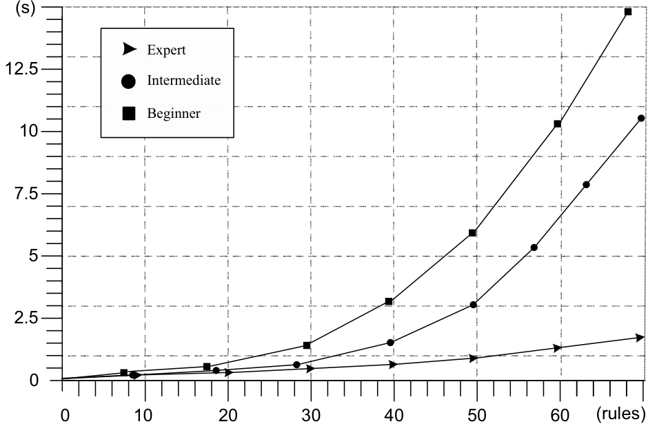
Inspired by the experiments done in [2, 3], we simulated in a first phase several sets of IPv4 filtering policies, according to the three following security officer profiles: beginner, intermediate, and expert – where the probability to have overlaps between rules increases from 5% to 90%. Then, we processed in a second phase all these sets of filtering rules within our prototype, in order to evaluate its performance and scalability.

Refer to caption — Figure 3: Memory space evaluation

The whole of these experiments were carried out on an Intel-Pentium M 1.4 GHz processor with 512 MB RAM, running Debian GNU/Linux 2.6.8, and using Apache/1.3 with PHP/4.3 interpreter configured. During these experiments, we measured the memory space and the processing time needed to perform algorithms 2, 3, and 4. The results of these measurements are plotted in Figure 3 and Figure 4. Although the plots reflect strong memory and process time requirements, we consider they are reasonable for off-line analysis, since it is not part of the critical performance of a firewall.

5 Conclusions

There are two ways to set a firewall configuration free of errors. A first approach is to apply a formal security model – such as the formal model presented in [5] – to express the security policy of the access control for the network, and to generate the specific syntax for each given firewall from this formal policy – for instance, by using XSL transformations from the formal policy to generate specific Netfilter configuration rules [10]. The main advantage of this approach is the great confidence we have in the conformity of the formal policy, and its translation into a specific firewall configuration. Nevertheless, although a great number of errors is avoided when using this formal approach, it is still not ensured that all the possible errors are discarded.

A second approach – as the one presented in this paper – is to apply an audit process to the set of filtering rules of a given firewall – which expresses a specific network security policy – in order to detect configuration errors and to properly eliminate them. In our case, the audit process is based on the existence of relationships between the condition attributes of the filtering rules, such as coincidence, disjunction, and inclusion. Then, our proposal uses a transformation process which derives from an initial set of rules – potentially misconfigured – to an equivalent one which is completely free of misconfiguration.

Some other advantages of our approach are the following. First of all, our transformation process verify that the resulting rules are completely independent between them. Otherwise, each redundant or shadowed rule considered as useless during the process is removed from the configuration. On the other hand, the discovering process provides an evidence of error to the administration console. This way, the security officer can check whether the security policy is consistent, in order to verify the correctness of the process.

The complete independence between rules, moreover, enables the possibility to perform a second rewriting of rules in a positive manner – only permissions – or in a negative manner – only prohibitions. After performing this second transformation, the security officer will have a clear view of the accepted traffic – when positive rewriting – or the rejected traffic – when negative rewriting.

Regarding a possible increase of the initial number of filtering rules, due to the applying of Algorithm 2, it is only significant whether the associated parsing algorithm of the firewall depends on the number of rules. In this case, an increase in such a parameter may degrade the performance of the firewall. Nonetheless, this is not a disadvantage since the use of a parsing algorithm independent of the number of rules becomes the best solution as much for our proposal as for the current deployment of firewall technologies. The set pruning tree algorithm is a proper example, because it only depends on the number and size of attributes to be parsed, not the number of rules [9].

The implementation of the algorithms in a software prototype demonstrate the practicability of our work. We shortly discussed this implementation, based on a general-purpose scripting language [4], and presented an evaluation of its performance. Although the experimental results show that our algorithms have strong memory and process time requirements, we believe that these requirements are reasonable for off-line analysis, since it is not part of the critical performance of a firewall.

As future work we are considering to extend our proposal to a more complex firewall setup. The work stated in this paper is based on the hypothesis that only one firewall ensures the network access control. More investigation has to be done when this role is assigned to more than one network security component, that is a distributed access control. Indeed, in particular, redundancy will not systematically be considered as an error [2]. It may be suited in order to avoid inconsistent decisions between firewalls used in the same security architecture to control the access to different zones.

In parallel to this work, we also study the anomaly problems of security rules in the case where the security architecture includes firewalls as well as IDS (Intrusion Detection Systems). The objective is to avoid redundant or shadowed filtering or/and alerting rules. Indeed, there is a real similarity between the parameters of a filtering rule and those of an alerting rules (signatures) so that we can apply algorithms presented in both Section 3.1 and Section 3.3. Of course, this will depend on whether the firewall is the first security component in the security architecture that the packets encounter or it acts after the detection intrusion component.

Acknowledgements

This work was supported by funding from the French ministry of research, under the ACI DESIRS project, the Spanish Government project TIC2003-02041, and the Catalan Government grants 2003FI126 and 2005BE77.

References

[1] Adiseshu, H., Suri, S., and Parulkar, G. (2000). Detecting and Resolving Packet Filter Conflicts. In 19th Annual Joint Conference of the IEEE Computer and Communications Societies (INFOCOM 2000), pages 1203–1212.
[2] Al-Shaer, E. S. and Hamed, H. H. (2004). Discovery of Policy Anomalies in Distributed Firewalls. In 23rd Annual Joint Conference of the IEEE Computer and Communications Societies (INFOCOM 2004).
[3] Al-Shaer, E. S., Hamed, H. H., and Masum, H. (2005). Conflict Classification and Analysis of Distributed Firewall Policies In IEEE Journal on Selected Areas in Communications, 1(1).
[4] Castagnetto, J., Rawat, H., Schumann, S., Scollo, C., and Veliath, D. (1999). Professional PHP Programming. Wrox Press Inc, ISBN 1-86100-296-3, 909 pages.
[5] Cuppens, F., Cuppens-Boulahia, N., Sans, T. and Miege, A. (2004). A formal approach to specify and deploy a network security policy. In Second Workshop on Formal Aspects in Security and Trust, pages 203–218.
[6] Cuppens, F., Cuppens-Boulahia, N., and García-Alfaro, J. (2005). Detection and Removal of Firewall Misconfiguration. In Proceedings of the 2005 IASTED International Conference on Communication, Network and Information Security (CNIS 2005).
[7] Gupta, P. (2000). Algorithms for Routing Lookups and Packet Classification. PhD Thesis, Department of Computer Science, Stanford University.
[8] Liu, A. X., Gouda, M. G., Ma, H. H., and Ngu, A. H. (2004). Firewall Queries. In Proceedings of the 8th International Conference on Principles of Distributed Systems (OPODIS-04), pages 197–212.
[9] Paul, O., Laurent, M., and Gombault, S. (2000). A full bandwidth ATM Firewall. In Proceedings of the 6th European Symposium on Research in Computer Security (ESORICS 2000), pages 206–221.
[10] Welte, H., Kadlecsik, J., Josefsson, M., McHardy, P., and et al. The netfilter project: firewalling, nat and packet mangling for linux 2.4x and 2.6.x. http://www.netfilter.org/

Appendix A Correctness Proofs

Proof of Lemma 3.2 Let us assume that:

$R_{i}[condition]=A_{1}\wedge A_{2}\wedge...\wedge A_{p}$ , and

$R_{j}[condition]=B_{1}\wedge B_{2}\wedge...\wedge B_{p}$ .

If $(A_{1}\cap B_{1})=\emptyset$ or $(A_{2}\cap B_{2})=\emptyset$ or …or $(A_{p}\cap B_{p})=\emptyset$ then $exclusion(R_{j},R_{i})\leftarrow R_{j}$ . Hence, to prove the equivalence between $\{R_{i},R_{j}\}$ and $\{R_{i},R^{\prime}_{j}\}$ is trivial in this case.

Let us now assume that:

$(A_{1}\cap B_{1})\neq\emptyset$ and $(A_{2}\cap B_{2})\neq\emptyset$ and … and $(A_{p}\cap B_{p})\neq\emptyset$ .

If we apply filtering rules $\{R_{i},R_{j}\}$ where $R_{i}$ comes before $R_{j}$ , then rule $R_{j}$ applies to a given packet if this packet satisfies $R_{j}[condition]$ but not $R_{i}[condition]$ (since rule $R_{i}$ applies first). Therefore, notice that $R_{j}[condition]-R_{i}[condition]$ is equivalent to:

$(B_{1}-A_{1})\wedge B_{2}\wedge...\wedge B_{p}$ or

$(A_{1}\cap B_{1})\wedge(B_{2}-A_{2})\wedge...\wedge B_{p}$ or

$(A_{1}\cap B_{1})\wedge(A_{2}\cap B_{2})\wedge(B_{3}-A_{3})\wedge...\wedge B_{p}$ or

$...$

$(A_{1}\cap B_{1})\wedge...\wedge(A_{p-1}\cap B_{p-1})\wedge(B_{p}-A_{p})$

which corresponds to condition of rule $R^{\prime}_{j}=exclusion(R_{j},R_{i})$ . This way, if rule $R_{j}$ applies to a given packet in $\{R_{i},R_{j}\}$ , then rule $R^{\prime}_{j}$ also applies to this packet in $\{R_{i},R^{\prime}_{j}\}$ .

Conversely, if rule $R^{\prime}_{j}$ applies to a given packet in $\{R_{i},R^{\prime}_{j}\}$ , then this means this packet satisfies $R_{j}[condition]$ but not $R_{i}[condition]$ . So, it is clear that rule $R_{j}$ also applies to this packet in $\{R_{i},R_{j}\}$ .

Since in Algorithm 2 $R^{\prime}_{j}[decision]$ becomes $R_{j}[decision]$ , this enables to conclude that $\{R_{i},R_{j}\}$ is equivalent to $\{R_{i},R^{\prime}_{j}\}$ . $\square$

Proof of Theorem 3.3 Notice that if $R$ is a set of filtering rules, then $Tr(R)$ is obtained by recursively applying transformation $exclusion(R_{j},R_{i})$ when rule $R_{i}$ comes before rule $R_{j}$ , which preserves the equivalence at each step of the transformation, previously proved for Lemma 3.2. $\square$

Proof of Lemma 3.4 Notice that rule $R^{\prime}_{j}$ only applies when rule $R_{i}$ does not apply. Thus, if rule $R^{\prime}_{j}$ comes before rule $R_{i}$ , this will not change the final decision since rule $R^{\prime}_{j}$ only applies to packets that do not match rule $R_{i}$ . $\square$

Proof of Theorem 3.5 For any pair of rules $R_{i}$ and $R_{j}$ such that $R_{i}$ comes before $R_{j}$ , $R_{j}$ is replaced by a rule $R^{\prime}_{j}$ obtained by recursively replacing $R_{j}$ by $exclusion(R_{j},R_{k})$ for any $k<j$ .

Then, by recursively applying Lemma 3.4, it is possible to commute rules $R^{\prime}_{i}$ and $R^{\prime}_{j}$ in $Tr(R)$ without changing the final decision. $\square$

Proof of Theorem 3.6 Notice that, in $Tr(R)$ , each rule is independent of all other rules. Thus, if we consider a rule $R_{i}$ in $Tr(R)$ such that $R_{i}[condition]\neq\emptyset$ , then this rule will apply to any packet that satisfies $R_{i}[condition]$ . Hence, this rule is not shadowed.

Similarly, rule $R_{i}$ is not redundant because if we remove this rule, since this rule is the only one that applies to packets that satisfy $R_{i}[condition]$ , then the filtering decision will change if we remove rule $R_{i}$ from $Tr(R)$ . $\square$

Proof of Theorem 3.7 Let $Tr^{\prime}_{1}(R)$ be the set of rules obtained after applying the first phase of Algorithm 4. Since $Tr^{\prime}_{1}(R)$ is derived from $R$ by applying $exclusion(R_{j},R_{i})$ (cf. Algorithm 2) to some rules $R_{j}$ in $R$ , it is straightforward, from Lemma 3.2, to conclude that $Tr^{\prime}_{1}(R)$ is equivalent to $R$ .

Hence, let us now move to the second phase of Algorithm 4. Let us consider a rule $R_{i}$ such that $testRedundancy(R_{i})$ (cf. Algorithm 3) is $true$ . This means that $R_{i}[condition]$ can be derived by conditions of a set of rules $S$ with the same decision and that come after in order than rule $R_{i}$ .

Since every rule $R_{j}$ with a decision different from the one of rules in $S$ has already been excluded from rules of $S$ in the first phase of the Algorithm, we can conclude that rule $R_{i}$ is definitely redundant and can be removed without changing the final filtering decision. This way, we conclude that Algorithm 4 preserves equivalence in this case.

On the other hand, if $testRedundancy(R_{i})$ is $false$ , then transformation consists in applying $exclusion(R_{j},R_{i})$ to some rules $R_{j}$ which also preserves equivalence. Thus, in both cases, $Tr^{\prime}(R)$ is equivalent to $Tr^{\prime}_{1}(R)$ which, in turn, is equivalent to $R$ . $\square$

Proof of Theorem 3.8 and Theorem 3.9 As stated out in the proof of both Theorem 3.5 and Theorem 3.6, once shadowed and redundant rules have been removed, every rule $R_{i}$ is replaced by $exclusion(R_{i},R_{j})$ where $j<i$ .

Therefore, a similar reasoning enables to prove both Theorem 3.8 and Theorem 3.9. $\square$

MISCONFIGURATION MANAGEMENT OF NETWORK SECURITY COMPONENTS

Abstract

1 Introduction

Definition 1.1

Definition 1.2

2 Related Work

3 Proposed Algorithms

3.1 Detection Process

3.1.1 Applying the Algorithms

3.2 Correctness of the Algorithms

Definition 3.1

Lemma 3.2

Theorem 3.3

Lemma 3.4

Theorem 3.5

Theorem 3.6

3.3 Complete Detection

3.3.1 Applying the Algorithms

3.4 Correctness of the Algorithms

Theorem 3.7

Theorem 3.8

Theorem 3.9

3.5 Complexity of the Algorithms

4 Performance Evaluation

5 Conclusions

Acknowledgements

References

Appendix A Correctness Proofs

MISCONFIGURATION MANAGEMENT
OF NETWORK SECURITY COMPONENTS