Single Image Deraining: From Model-Based to Data-Driven and BeyondThanks: Wenhan Yang and Shiqi Wang are with Department of Computer Science, City University of Hong Kong, Hong Kong, China, (e-mail: {wyang34, shiqwang}@cityu.edu.hk). Robby T. Tan is with Yale-NUS College and the Department of Electrical and Computer Engineering, National University of Singapore, Singapore, (e-mail: tanrobby@gmail.com). Yuming Fang is with the School of Information Management, Jiangxi University of Finance and Economics, Jiangxi, China, (e-mail: fa0001ng@e.ntu.edu.sg). Jiaying Liu is with Wangxuan Institute of Computer Technology, Peking University, Beijing, China, (e-mail: liujiaying@pku.edu.cn).
Abstract
The goal of single-image deraining is to restore the rain-free background scenes of an image degraded by rain streaks and rain accumulation. The early single-image deraining methods employ a cost function, where various priors are developed to represent the properties of rain and background layers. Since 2017, single-image deraining methods step into a deep-learning era, and exploit various types of networks, i.e. convolutional neural networks, recurrent neural networks, generative adversarial networks, etc., demonstrating impressive performance. Given the current rapid development, in this paper, we provide a comprehensive survey of deraining methods over the last decade. We summarize the rain appearance models, and discuss two categories of deraining approaches: model-based and data-driven approaches. For the former, we organize the literature based on their basic models and priors. For the latter, we discuss developed ideas related to architectures, constraints, loss functions, and training datasets. We present milestones of single-image deraining methods, review a broad selection of previous works in different categories, and provide insights on the historical development route from the model-based to data-driven methods. We also summarize performance comparisons quantitatively and qualitatively. Beyond discussing the technicality of deraining methods, we also discuss the future directions.
Index Terms:
Rain streak removal, single image, model-based, data-driven, surveyI Introduction
Rain introduces visual degradations to captured images and videos. Rain streaks particularly in heavy rain can cause severe occlusion on the background scene. Rain accumulation [1], where distant rain streaks cannot be seen individually and together with water particles form a layer of veil on the background, significantly degrades the contrast of the scene and reduce the visibility. Fig. 1 shows examples of degradation due to rain streaks and rain accumulation. Human vision and many computer vision algorithms suffer from this degradation, since most of these algorithms assume clear weather, with no interference of rain streaks and rain accumulation. Hence, restoring images from rain, called deraining or rain removal, is much desired in many practical applications.
An early study of video deraining was started in 2004 by Garg and Nayar [3]. They analyze rain dynamic appearances, and develop an approach to remove rain streaks from videos. Kang et al. [4] was a pioneer in the single image deraining by publishing a method in 2012. The method extracts the high-frequency layer of a rain image, and decomposes the layer further into rain and non-rain components using dictionary learning and sparse coding. Starting from 2017, by the publications of [1, 18], data-driven deep-learning methods that learn features automatically become dominant in the literature.


In this survey, we focus on single-image deraining, which the aim is to estimate the rain-free background layer of an image degraded by rain streaks and rain accumulation. Unlike video deraining methods, which leverage temporal redundancy and dynamics of rain, single image deraining methods exploit the spatial information of neighboring pixels and the visual properties of rain and background scenes.
The milestones of single-image deraining in the past years are presented in Fig. 2. Before 2017, the typical methods are model-based approach (or non-deep learning approach). The major developments in the model-based approach are driven by the following ideas: image decomposition (2012), sparse coding (2015), and priors based Gaussian mixture models (2016). Since 2017, single-image deraining methods enter into a period of data-driven approach (or deep learning approach). The major developments in the data-driven approach are indicated by the following ideas: deep convolutional network (2017), generative adversarial network (2019), and semi/unsupervised methods (2019). In 2017-2019, there are more than 30 papers on this deep learning approach, significantly more than the number of deraining papers before 2017.
Model-based methods rely more on the statistical analysis of rain streaks and background scenes. The methods enforce handcrafted priors on both rain and background layers, then build a cost function and optimize it. The priors are extracted from various ways: Luo et al. [5] learn dictionaries for both rain streak and background layers, Li et al. [6] build Gaussian mixture models from clean images to model background scenes, and from rain patches of the input image to model rain streaks, Zhu et al. [7] enforce a certain rain direction based on rain-dominated regions so that the background textures can be differentiated from rain streaks.
In recent years, the popularity of data-driven methods has overtaken model-based methods. These methods exploits deep networks to automatically extract hierarchical features, enabling them to model more complicated mappings from rain images to clean ones. Some rain-related constraints are usually injected into the networks to learn more effective features, such as rain masks [1], background features [8], etc. Architecture wise, some methods utilize recurrent network [1], or recursive network [9] to remove rain progressively. There are also a series of works focusing on the hierarchical information of deep features, e.g. [10, 11].
While deep networks lead to a rapid progress in deraining performance, many of these deep-learning deraining methods train the networks in a fully supervised way. This can cause a problem, since to obtain paired images of rain and rain-free images is intractable. The simplest solution is to utilize synthetic images. Yet, there are domain gaps between synthetic rain and real rain images, which can make the deraining performance not optimum. To overcome the problem, unsupervised/semi-supervised methods that exploit real rain images [12] and [13] are introduced.
Our paper aims to provide a comprehensive survey on single-image deraining methods. We believe it can provide a useful starting point to understand the main development of the field, the limitations of existing methods, and the possible future directions. The rest of the paper is organized as follows. Section II introduces the rain appearance model. Section III provides a detailed survey of single-image rain removal methods, including their synthetic rain models, deraining challenges, methods architectures, and the related technical development. A particular emphasis is placed on the deep-learning based methods as they offer the most significant progress in the recent years. Subsequently, Section IV gives detailed discussion on technical developments of network architectures, basic blocks, and summaries of loss functions and databases. Section V summarizes the quantitative comparisons of a number of single-image rain removal methods and shows qualitative comparisons. Finally, the paper is concluded in Section VI.
II Raindrop Appearance Models
The shape of a raindrop is usually approximated by a spherical shape [14]. As shown in Fig. 3, considering a point B on the surface of the raindrop with a surface normal , rays of light (, and ) are directed toward the observer via refraction, specular reflection, and internal reflection, respectively. Hence, the radiance at point B is approximated as the sum of the radiance of refracted ray, radiance of specularly reflected ray and radiance of internally reflected ray:
| (1) |
Considering that the radiances depend on the environmental radiance in the direction of the reflected or refracted ray, Eq. (1) can be expressed as:
| (2) |
where , and denote the fractions of incident environmental radiance that reaches the camera after refraction, reflection and internal reflection, respectively. We refer to these fractions as radiance transfer functions.
Moreover, we can reach the composite raindrop model written as [14]:
| (3) |
where is the incident angle, is the refractive index of the water and is the Fresnel’s reflectivity coefficient for unpolarized light. Based on the statistics from [14], the radiance of the raindrop is mainly decided by the refraction, and the appearance of the raindrop is mainly based on refraction through the drop.
For a moving raindrop, its appearance changes significantly. The raindrop becomes a rain streak, and its appearance relies on the brightness of the raindrop, background scene radiances, and camera’s exposure time. The change of pixel’s intensity value caused by a rain streak can be approximated as [14]:
| (4) |
with , and , where is the time when a drop remains within a pixel, and is the exposure time. is the time-averaged irradiance caused by the drop. Based on Eq. (4), we can reach two conclusions: 1) A raindrop causes an intensity change and moves faster than the integration time of a typical video camera; 2) the intensity change of a rain streak correlates linearly to the background intensity . Based on the derived numerical bounds [14], empirically we obtain: and . In most real cases, dominates the appearance of , thus:
| (5) |
As a result, in most rain synthetic models, rain streaks are assumed to be superimposed on the background image.
| Method | Degradation Factors | Main Features | Publication | ||
|---|---|---|---|---|---|
| Additive Composite Model (ACM) | Streak | Simple and effective | Li et al. 2016 [6] | ||
| Screen Blend Model (SBM) | Streak | Streaks and backgrounds are combined nonlinearly | Luo et al. 2015 [5] | ||
| Heavy Rain Model (HRM) | Streak, Accumulation | Overlapping streaks generating accumulation | Yang et al. 2017 [1] | ||
| Rain Model with Occlusion (ROM) | Streak, Occlusion | Considering rain occlusions | Liu et al. 2018 [15] | ||
| Comprehensive Rain Removal (CRM) |
|
Considering comprehensive visual degradation | Yang et al. 2019 [2] | ||
| Depth-Aware Rain Model (DARM) | Streak, Accumulation | Streaks and accumlation modeling correlated with depth | Hu et al. 2019 [16] |
III Literature Survey
In this section, we first review a few rain synthesis models proposed in some existing methods. Unlike in the previous section (Sec. II), the models we discuss here are only loosely based on physics and thus, to our knowledge, their correctness has not been verified both theoretically or experimentally. Despite this, the methods that use these models show, to some extent, the effectiveness of the models on real-image deraining. Having discussed various rain synthetic models, we briefly explain the challenges in image deraining, and subsequently survey on existing deraining methods comprehensively.
III-A Synthetic Rain Models
Additive Composite Model The most simple and popular rain model used in existing studies is the additive composite model [6, 4], which follows Eq. (5) and is expressed as:
| (6) |
where denotes the background layer, and is the rain streak layer. is the image degraded by rain streaks. Here, the model assumes that the appearance of rain streaks is simply superimposed to the background, and there is no rain accumulation in the rain degraded image.
Screen Blend Model Luo et al. [5] propose a non-linear composite model, called screen-blend model:
| (7) |
where denotes the operation of point-wise multiplication. Unlike the additive composite model in Eq. (6), the background and rain layers influence the appearance of each other. Luo et al. [5] claim that the screen blend model can model some visual properties of real rain images, such as the effect of internal reflections, and thus generate visually more authentic rain images. The combination of rain and background layers are signal-dependent. Implying, when the background is dim, the rain layer will dominate the appearance of the rain image; and, when the background is bright, the background layer will dominate the image.
Heavy Rain Model Yang et al. [1] propose a rain model that includes both rain streaks and rain accumulation. This is the first model in the deraining literature that includes the two rain phenomena. Rain accumulation or rain veiling effect is a result of water particles in the atmosphere and distant rain-streaks that cannot be seen individually. The visual effect of rain accumulation is similar to mist or fog, which leads to low contrast. Considering two main aspects of rain: the Koschmieder model to approximate the visual appearance of a scene in a turbid medium, and overlapping rain streaks that have different directions and shapes, a novel rain model is introduced:
| (8) |
where denotes the rain-streak layer that has the same streak direction. indexes the rain-streak layer and is the maximum number of the rain-streak layers. A is the global atmospheric light, and is the atmospheric transmission.
Rain Model with Occlusion Liu et al. [15] extend the heavy rain model to an occlusion-aware rain model for modeling rain in video. The model separates rain streaks into two types: transparent rain streaks that are added to the background layers, and opaque rain streaks that totally occlude the background layers. The locations of these opaque rain streaks are indicated by a map, called the reliance map. The formulation of this rain model is expressed as:
| (9) |
where R is the rain reliance map and is defined as:
| (10) |
where is defined as the rain occluded region.
Comprehensive Rain Model Yang et al. [2] combine all above mentioned degradation factors into a comprehensive rain model for modeling rain appearance in video. It considers the temporal properties of rain scenes, particularly the fast-changing rain accumulations that usually cause flicker. This visible intensity changes along the temporal dimension is called rain accumulation flow. Besides, it also considers other factors including rain streaks, rain accumulation, and rain occlusion, which are formulated as:
| (11) |
where is the rain accumulation flow.
Depth-Aware Rain Model Hu et al. [16] further connect to the scene depth , to create a depth-aware rain model:
| (12) |
where and are connected with the scene depth written as:
| (13) | ||||
where is an intensity image of uniformly-distributed rain streaks in the image space, and is the rain streak intensity map relying on the depth. denotes the depth and controls the rain streak intensity. determines the thickness of fog, where a larger denotes a thicker fog.
Discussions Following these different rain models, various rain degradation can be synthetically rendered. A summary of rain synthetic models in the literature is provided in Table I. In general, heavy rain models [1, 13] and depth-aware rain models [16] cover the most comprehensive rain degradation for single rain image synthesis. However, as we mentioned in the beginning of this section that all these models are heuristic; implying that they might not entirely correct physically. Nevertheless, as shown in the literature, they can be effective, at least to some extent, for image deraining.
III-B Deraining Challenges
The goal of single image deraining is to recover the clean and rain-free background scene from a rain degraded image. However, there are a few challenges to accomplish the goal:
- •
Difficulties in modeling rain images In the real world, rain can visually appear in many different ways. Rain streaks can vary in terms of sizes, shapes, scales, densities, directions, etc. Similarly, rain accumulation depends on various water-particles and atmospheric conditions. Moreover, rain appearance significantly relies also on the textures and the depth of the background scenes. All these cause difficulties in modeling the appearance of rain, which consequently cause the rendering of physically-correct rain images to be a complex task.
- •
Ill-posedness of deraining problem Even with a simple rain model that considers only rain-streaks, to estimate the background scene from a degraded image is an ill-posed problem. The reason is that we only have the pixel intensity values produced by lights carrying fused information of rain and background scenes. To make the matter worse, in some cases the background information can be totally occluded by rain streaks or dense rain accumulation or both.
- •
Difficulties in finding proper priors As rain and background information might overlap in the feature space, it is non-trivial to separate them. Background textures can be falsely deemed as rain, resulting in incorrect deraining. Hence, strong priors for background textures and rain are necessary. However, finding these priors is difficult, since background textures are diverse, and some have similarity to the appearance of rain-streaks or rain accumulation.
- •
Real paired ground-truths Most of deep-learning methods rely on paired rain and clean background images to train their networks. However, to obtain real rain images and their exact pairs of clean background images is intractable. Even for a static background, lighting conditions always change. This difficulty does not only impact on deep-learning methods, but also for evaluating the effectiveness of any method. Currently, for qualitative evaluation, all methods rely on human subjective judgment on whether the restored images are good; and for quantitative evaluation, all current methods rely on synthetic images. Unfortunately, up to now, there are significant gaps between synthetic and real images.
In the following section, we will discuss how existing deraining methods deal with these challenges.

III-C Single-image Deraining Methods
We categorize single-image deraining methods into two basic approaches: model-based (non-deep-learning) and data-driven (deep-learning) approaches. We will discuss the existing methods of the two approaches in detail in the subsequent sections. A summary of previous works is given in Table II. In addition, for the sake of completeness, we will also briefly discuss adherent raindrop removal methods, since adherent raindrops (i.e., water droplets attached to a lens or windscreen) are also part of rain degradation; although, in some situations, they can be avoided by placing the camera under a shelter.
| Method | Category | Rain Model |
|
Key Idea | Publication | ||||||||||
|---|---|---|---|---|---|---|---|---|---|---|---|---|---|---|---|
| Image Decomposition | Sparse Representation | ACM |
|
|
Kang et al. 2012 [4] | ||||||||||
| DSC | SBM |
|
|
Luo et al. 2015 [5] | |||||||||||
| Bi-Layer Optimization | ACM |
|
|
Zhu et al. 2017 [7] | |||||||||||
| Hierarchical Deraining | ACM |
|
|
Wang et al. 2017 [32] | |||||||||||
| DGSM | ACM |
|
|
Deng et al. 2018 [17] | |||||||||||
| LP | GMM | ACM |
|
|
Li et al. 2016 [6] | ||||||||||
| CNN | Deep CNN | Raindrop | Clean image. |
|
Eigen et al. 2013 [27] | ||||||||||
|
HRM |
|
|
| |||||||||||
| DetailNet | ACM | Residual. |
|
| |||||||||||
| Scale-Aware | HRM |
|
|
Li et al. 2017 [20] | |||||||||||
| NLEDN | ACM | Residual. |
|
Li et al. 2018 [10] | |||||||||||
| Residual-Guide | ACM | Residual. |
|
Fan et al. 2018 [8] | |||||||||||
| RESCAN | ACM |
|
|
Li et al. 2018 [21] | |||||||||||
| DID-MDN | ACM |
|
|
Zhang et al. 2018 [22] | |||||||||||
| DualCNN | ACM |
|
|
Pan et al. 2018 [23] | |||||||||||
| DAF-Net | DARM |
|
|
Hu et al. 2019 [16] | |||||||||||
|
ACM |
|
|
Wang et al. 2019 [34] | |||||||||||
| PReNet | ACM |
|
|
Ren et al. 2019 [9] | |||||||||||
| Scale-Free | HRM |
|
|
Yang et al. 2019 [30] | |||||||||||
| PyramidDerain | ACM |
|
|
Fu et al. 2019 [11] | |||||||||||
| UMRL | ACM |
|
|
Yasarla et al. 2019 [29] | |||||||||||
| AttGAN | GAN | Raindrop |
|
|
Qian et al. 2018 [28] | ||||||||||
| CGAN | ACM | Clean image. |
|
Zhang et al. 2019 [24] | |||||||||||
| HeavyRainRestorer | HRM |
|
|
Li et al. 2019 [13] | |||||||||||
| Semi-supervised CNN | Semi/Un- Supervised | ACM |
|
|
Wei et al. 2019 [25] | ||||||||||
| UD-GAN | ACM |
|
|
Jin et al. 2019 [12] | |||||||||||
| Benchmark | Benchmark |
|
– |
|
Li et al. 2019 [26] |
III-C1 Model-based Methods
Existing model-based methods employ optimization frameworks for deraining, as shown in the top panel of Fig. 4. These methods deal only with rain streaks and ignore the presence of rain accumulation. A general optimization framework can be expressed as:
| (14) |
where denotes the priors on the background layers, represents the priors on rain streak layers, and is the joint prior to describe the intrinsic relationship between rain streaks and background layers. Different prior terms are designed to better describe and separate the rain streak from the background layers.
Sparse Coding Methods Sparse coding [56] represents the input vectors as a sparse linear combination of basis vectors. The collection of these basis vectors is called dictionary, which is used to reconstruct the certain type of signals, e.g. rain streaks and background signals in the deraining problem. Lin et al. [4] make the first attempt on single-image deraining via image decomposition using a morphological component analysis. The initially extracted high-frequency component of a rain image is further decomposed into rain and non-rain components by dictionary learning and sparse coding. This pioneer work successfully removes sparse light rain streaks. However, it significantly relies on the bilateral filter preprocessing, and thus generates blurred background details.
In a successive work, Luo et al. [5] enforce the sparsity of rain, and introduce a mutual exclusivity property into a discriminative sparse coding (DSC) to facilitate accurately the separation of the rain/background layers from their non-linear composite. Benefiting from the mutual exclusivity property, the DSC preserves clean texture details; however, it shows some residual rain streaks in the output, particularly for large and dense rain streaks. To further improve the modeling capacity, Zhu et al. [7] construct an iterative layer separation process to remove rain streaks from the background layer, as well as to remove background’s texture details from the rain streak layer using layer-specific priors. Quantitatively, the method obtains comparable performance on some synthetic datasets with that of deep learning-based methods published in the same period of time, i.e. JORDER [1] and DDN [18]. However, qualitatively on real images, the method tends to fail in handling heavy rain cases, where rain streaks may move in different directions.
To model rain streak directions and sparsity, Deng et al. [17] formulate a directional group sparse model (DGSM), which includes three sparse terms representing the intrinsic directional and structural knowledge of rain streaks. It can effectively remove blurred rain streaks but fail to remove sharp rain streaks.
Gaussian Mixture Model Li et al. [6] apply Gaussian mixture models (GMMs) to model both rain and background layers. The GMMs of the background layer is obtained off-line from real images with diverse background scenes. A selected rain patch from the input image that has no background textures is proposed to train the GMMs of the rain layer. The total variation is utilized to remove small sparkle rains. The method is capable to effectively remove rain streaks of small and moderate scales, but fail to handle large and sharp rain streaks.
III-C2 Deep Learning Based Methods
Deep CNNs The era of deep-learning deraining starts in year 2017. Yang et al. [1] construct a joint rain detection and removal network. It can handle heavy rain, overlapping rain streaks, and rain accumulation. The network can detect rain locations by predicting the binary rain mask, and take a recurrent framework to remove rain streaks and clear up rain accumulation progressively. The method achieves good results in heavy rain cases. However, it might falsely remove vertical textures and generate underexposed illumination.
In the same year, Fu et al. [18, 19] made an attempt to remove rain streaks via a deep detail network (DetailNet). The network takes only the high frequency details as input, and predicts the residue of the rain and clean images. The paper shows that removing the background information in the network input is beneficial, as doing so makes the training easier and more stable. However, the method still cannot handle large and sharp rain streaks.
Following Yang et al. [1] and Fu et al. [18, 19], many CNN based methods [20, 10, 8, 21, 22, 23] are proposed. These methods employ more advanced network architectures and injecting new rain related priors. They achieve better results both quantitatively and qualitatively. However, due to the limitation of their fully supervised learning paradigm, namely using synthetic rain images, they tend to fail when dealing with some conditions of real rain that has never been seen during training.


Generative Adversarial Networks To capture some visual properties of rain that cannot be modeled and synthesized, the adversarial learning is introduced to reduce the domain gaps between the generated results and real clean images. The typical network architecture consists of two parts: generator and discriminator, where the discriminator attempts to assess whether a generated result is real or fake, which provides an additional feedback to regularize the generator to produce more visually pleasing results. Zhang et al. [24] directly apply the conditional generative adversarial network (CGAN) for the single image rain removal task, as shown in Fig. 5 (a). CGAN is capable of capturing the visual properties beyond the signal fidelity, and presents results with better illumination, color and contrast distribution. However, CGAN sometimes might generate visual artifacts when the background of the testing rain image is different from those in the training set.
Li et al. [13] propose a single-image deraining method that combines the physics-driven network and adversarial learning refinement network, as shown in Fig. 5 (c). The first stage learns from the synthesized data and estimates physics-related components, i.e. rain streaks, the transmission, and the atmospheric light. At the second refinement stage, a depth-guided GAN is proposed to compensate for the lost details and to suppress the introduced artifacts at the first stage. Learning from real rain data, some visual properties of the results by these methods are significantly improved, namely removing rain accumulation more thoroughly and achieving a more balanced luminance distribution. However, as GAN-based methods are not good at capturing fine-grained detail signals, the diversified appearances of real rain streaks are also not properly modeled in these methods.
Semi/Unsupervised Learning Methods Recently, semi-supervised and unsupervised learning methods make an attempt to improve the generality and scalability by learning directly from real rain data. Wei et al. [25] propose a semi-supervised learning method to make use of the priors in both synthesized paired data and unpaired real data, as shown in Fig. 6 (a). In the proposed method, the residual is formulated as a specific parametrized rain streak distribution between an input rain image and its expected network output. The model trained on synthesized paired rain images is adapted to handle diversified rain in real scenarios with the guidance of the rain-streak distribution model. The method, however, does not show effective deraining results particularly for real rain images. This might be caused by the loose loss functions they impose to the network during the training process.
In [12], an unsupervised deraining generative adversarial network (UD-GAN) is proposed by introducing self-supervised constraints, and the intrinsic priors extracted from unpaired rain and clean images, as shown in Fig. 6 (b). Two collaborative modules are designed: One module is utilized to detect the difference between real rain images (real background images) and generated rain images (generated background images); while the other is introduced to adjust the luminance of the generated results, making the results more visually pleasing. The method is capable of removing real rain from rain images, yet inevitably losing some details, particularly when the rain streaks are dense.
Benchmark Li et al. [26] provided extensive study and evaluation of existing single image deraining algorithms with a newly proposed large-scale dataset including both synthetic and real-world rain images with various rain types, i.e. rain streak, raindrops, and mist. The benchmark also includes a wide range of evaluation criteria including the results of different methods quantitatively and qualitatively.
III-C3 Adherent Raindrop Removal
Raindrops adhered to the camera lens can severely degrade visibility of a background scene in an image. The goal of adherent raindrop removal is to detect and remove raindrops from an input image. Deraining is different from adherent raindrop removal, since rain images do not always suffer from adherent raindrop degradation, and vice versa: Adherent raindrop images do not always suffer from the degradation of rain streaks or rain accumulation. Nevertheless, we discuss it briefly here for the sake of the completeness of the survey.
In [57], Yamashita et al. develop a stereo system to detect and remove raindrops. Subsequently, a method [58] is built based on the image sequence instead of stereo video. You et al. [59] propose a motion based method to detect raindrops, and apply video completion to remove the detected regions. Eigen et al. [27] make the first attempt to tackle the problem of single-image raindrop removal. A three-layer CNN is trained with pairs of raindrop degraded images and the corresponding clean ones. It can handle relatively sparse and small raindrops as well as dirt, however, it fails to produce clean results for large and dense raindrops.
Recently, Qian et al. [28] develop an attentive GAN (AttGAN) [28] by injecting visual attention into both the generative and discriminative networks, as shown in Fig. 5 (b). The visual attention does not only guide the discriminative network to focus more on local consistency of the restored raindrop regions, but also make the generative network pay more attention to the contextual information surrounding the raindrop areas.
IV Technical Development Review
In this section, we summarize the developments of existing deep-learning methods from the perspective of the network architectures, basic blocks, loss functions, and datasets. These aspects significantly influence the network’s learning capacity and thus determine the networks’ deraining performance.

IV-A Network Architectures
Since the publications of deep learning based deraining [19, 1], the successive methods aim to design more effective network architectures by relying on certain assumptions/constraints and general knowledge in image processing. In this section, we take a look at these developments.
| Side information | Methods |
|---|---|
| Rain Mask | JORDER [1] |
| Rain Density | JORDER [1], DID-MDN [22] |
| Depth | DAF-Net [16], HeavyRainRestorer [13] |
| Attention | DAF-Net [16], SPA-Net [34], AttGAN [28] |
| Intermediate Results | JORDER-E [33], PReNet [9], |
| Bands Results | Scale-Free Rain Removal [30], PyramidNet [11] |
Deraining Assumptions/Constraints Specific networks dedicated to certain problems usually perform better than generic networks. To create these specific networks, some constraints or assumptions about the problems need to be injected. For deraining, these assumptions can relate to rain, background scenes, or other information. By incorporating some of these assumptions, a network is expected to learn the characteristics of rain better, and thus to separate rain layer from the background layer more robustly.
Fu et al. [19] assume a rain image can be decomposed into detail and base layers, where the detail layer contains the image textures and rain streaks (Fig. 7 (a)), and the base layer mostly contains the background and the rain accumulation. The proposed network thus attempts to derain the the detail layer, before fusing the layer with the base layer to obtain the rain-free output.
Yang et al. [1] construct a joint rain detection and removal network as shown in Fig. 7 (b) to detect rain locations, estimate rain densities and predict rain sequentially, which boosts the capacity of the network to process rain and non-rain regions differently. Li et al. [20] focus on the scale diversity of rain streaks. A scale-aware network as shown in Fig. 7 (c) consisting of parallel subnetworks is built to make it aware of different scales of rain streaks, producing better deraining performance for real images. Zhang et al. [22] propose a density-aware rain removal method (DID-MDN) as shown in Fig. 7 (d) to automatically detect the rain-density as the guidance information for the successive deraining.
Aside from assumptions related to rain, some assumptions ar related to the background scenes. Hu et al. [16] analyze the complex visual effects in real rain and formulate a rain imaging model related to the scene depth. An end-to-end deep neural network as shown in Fig. 7 (e) is developed to extract depth-attentional features and to regress a residual map for predicting the clean image. In [23], a dual CNN as shown in Fig. 7 (f) is presented, where two branches learn the estimation of two parts of the target signal: structures and details.
Another type of constraints is the confidence information of the residual between the estimated background layer and the ground-truth. In Fig. 7 (g), the model [29] learns about rain streaks by being guided by a per-pixel confidence map. This map is used to weigh wrongly estimated pixels in the back-propagation process, so that the network can pay more attention to these pixels during the training process. A summary of deraining side information used in previous works in provided in Table III.
Image Processing Knowledge Some ideas present in the image processing literature can also useful in designing deraining network architectures, for instance: multi-scale structure, Laplacian pyramid, wavelet transform, etc.. A scale-free network [30] as shown in Fig. 8(a) pays attention to the scale variety of rain streaks in real scenes, and constructs a scale-free deraining architecture by unrolling a wavelet transform into a recurrent neural network, which can handle various kinds of rain at different scales. Guided by the hierarchical representation of the wavelet transform, a recurrent network consisting of two stages is built: 1) rain removal on the low-frequency component; 2) recurrent detail recovery on high-frequency components gudied by the recovered low-frequency component.
PyramidDerain [11] pursues a light-weighted pyramid of network as shown in Fig. 8(b) to remove rain from a single image. The decomposed Gaussian Laplacian image pyramid is combined with a deep network. The learning paradigm at each pyramid layer can be simplified, and the obtained network becomes shallow and has less parameters. The model is quite light-weighed and achieves comparable state-of-the-art performance.
Li et al. [31] propose a recurrent network to remove rain streaks progressively as shown in Fig. 8(c). The intermediate result from the last recurrence is taken as the input of the next recurrence, and the features are also forwarded and fused by RNN units, e.g. GRU and LSTM, across recurrences. Ren et al. [9] utilize recursive computation to obtain more effective processing as shown in Fig. 8(d). The PReNet performs stage-wise operations that process the input and intermediate results to generate the clean output images progressively.
IV-B Basic Blocks
With the development of deep-learning based methods, the trend of newly proposed methods is to have more complex basic blocks with more powerful modeling capacities, which are further stacked into a more complex deraining network.
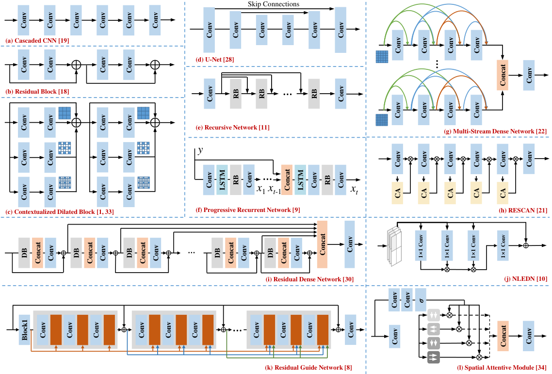
Using Existing Architectures DetailNet [18, 19] (Fig. 9 (a) and (b)) introduces a residual network and a cascaded CNN for rain removal. AttGAN [28] (Fig. 9 (d)) utilizes U-Net as the baseline of the generator, which is effective to fuse the information from different scales to obtain global information while maintaining local details. RESCAN [31] (Fig. 9 (h)) introduces channel-wise attention to adjust the relative weighting among channels for better separating rain streaks from background layers.
Multi-stream dense network [22] (Fig. 9 (g)) combines dense block and convolutional networks. Residual dense network [30] (Fig. 9 (i)) integrates dense blocks into residual networks. In [8] (Fig. 9 (k) and (e)), basic blocks are connected in the recursive way, where the input feature is also forwarded to the intermediate features of the network. In [9] (Fig. 9 (f)), residual blocks are also aggregated in the recursive way and the LSTMs are selected to connect different recurrences.
Multi-Path Architectures One of the common architectures is the multi-path network. As shown in Fig. 9 (c), (g) and (l), the networks have different paths possessing different properties, i. e. kernel sizes, dilation factors, and filter directions, to gather different kinds of information. In Fig. 9 (c) and (e), different paths have different receptive fields, and thus can obtain both global information and maintain local structural details. In Fig. 9 (l), the spatial redundancies are aggregated from different directions to form visual attention.
Recursive Architectures In [8, 31, 9, 11], recursive blocks are nested and aggregated in the recursive way as shown in Fig. 9 (f), (k), (e) and (i). The networks perform stage-wise operations that process the input and intermediate results to generate the output clean images progressively. Inter-stage recursive computation of different blocks is sometimes adopted to propagate information across the blocks.
Non-locally enhanced encoder-decoder network [10] as shown in Fig. 9 (j) incorporates nonlocal operations to the design of an end-to-end network for deraining. The non-local operation calculates the feature at a spatial position as a weighted sum of the features at a specific range of positions. In [34], a spatial attentive module as shown in Fig. 9 (l) employs recurrent neural networks with ReLU and identity matrix initialization, to accumulate global contextual information in four directions. It utilizes another branch to capture the spatial contexts to selectively highlight the transformed rain features.
IV-C Loss Functions
In existing deraining methods, several loss functions have been proposed to regularize the training of the deraining network.
Fidelity-Driven Metrics Most studies need to use signal fidelity-driven matrices as the loss functions, such as Mean Squared Error (MSE) (L2), mean squared error (MAE) (L1), and SSIM [41]. They are defined as follows:
| (15) | ||||
| (16) | ||||
| (17) |
where and are the ground truth and predicted clean images. and are the average of and , respectively. and are the variance of and , respectively. and are two numbers to stabilize the division with weak denominator.
Rain-Related Loss The rain-related variable prediction loss makes some outputs of the network predict the rain-related variable. For example, in [1], the streak and the binary streak maps are connected to the corresponding losses as follows:
| (18) | ||||
where , , and are the ground truth rain streak, predicted rain streak, ground truth rain mask, and predicted rain mask, respectively. indexes the spatial pixel location.
Multi-Scale Loss The multi-scale loss [28] constrains the deraining network at different scales, which is expressed as:
| (19) |
where indexes the scale, and and are the down-sampled versions of and with the scaling factor .
Perception-Driven Loss Applying perceptual and adversarial losses [28] improves the perceptual quality of generated results. The perceptual loss is formulated as:
| (20) |
where is a pretrained CNN transformation. The adversarial loss used for deraining network is represented as:
| (21) |
where is a discriminator network that differentiates the generated and the ground truth . A summary of loss functions used in previous works is given in Table IV.
| Loss Function | Methods | |||||
|---|---|---|---|---|---|---|
| MSE (L2) |
| |||||
| MAE (L1) |
| |||||
| SSIM |
| |||||
| Adversarial | AttGAN [28], CGAN [24] | |||||
| Perceptual | AttGAN [28], DID-MDN [22], CGAN [24] | |||||
| Multi-Scale | AttGAN [28] | |||||
| Variable |
|
| Dataset |
|
Highlight | Rain Model | Publication | |||
|---|---|---|---|---|---|---|---|
| Rain12 | 12 |
|
ACM | Li et al. [6] | |||
| Rain100L | 1,800/100 |
|
ACM | Yang et al. [1] | |||
| Rain100H | 1,800/100 |
|
ACM | Yang et al. [1] | |||
| Rain800 | 700/100 |
|
ACM | Zhang et al. [24] | |||
| Rain14000 | 9,100/4,900 |
|
ACM | Fu et al. [18] | |||
| Rain12000 | 12,000/4000 |
|
ACM | Zhang et al. [22] | |||
| RealDataset | 28,500/1,000 |
|
ACM | Wang et al. [34] | |||
| NYU-Rain | 13,500/2,700 |
|
HRM | Li et al. [13] | |||
| Outdoor-Rain | 9,000/1,500 |
|
HRM | Li et al. [13] | |||
| RainCityscapes | 9,432/1,188 |
|
DARM | Hu et al. [16] | |||
| MPID | 1,561/419 |
|
ACM + HRM | Li et al. [26] |
IV-D Datasets
There are a few benchmarking datasets for image deraining, as introduced in Table V. These datasets are useful for network training as well as for evaluation:
- •
Rain12 [6] includes 12 synthesized rain images with only one type of rain streaks.
- •
Rain100L and Rain100H [1] include the synthesized rain images with only one type and five types of rain streaks, respectively.
- •
Rain800 [24]’s training set consists of a total of 700 images, where 500 images are randomly chosen from the first 800 images in the UCID dataset [36] and 200 images are randomly chosen from the BSD500’s training set [40]. The testing set consists of a total of 100 images, where 50 images are randomly chosen from the last 500 images in the UCID dataset and 50 images are randomly chosen from the testing set of the BSD-500 dataset.
- •
- •
Rain12000 [22] consists of 12,000 images in the training set, where each image is assigned a label based on its corresponding rain-density level (i.e. light, medium and heavy). There are 4,000 images per rain-density level in the dataset. The synthesized testing set includes 1,200 images.
- •
RealDataset [34] includes 29,500 rain/rain-free image pairs that cover a wide range of natural rain scenes, where the rain-free images are synthesized based on temporal redundancy and visual properties.
- •
NYU-Rain [13] is a new synthetic rain dataset taking images from NYU-Depth V2 [37] as background and the provided depth information to generate rain streak and accumulation layers. The dataset also considers the effect of image blurring presented in the rain image. It contains 16,200 image samples, where 13,500 images are used as the training set.
- •
- •
MPID [26]’s training set includes 2400 synthetic rain streak image pairs, 861 synthetic raindrop image pairs, and 700 synthetic rain and mist image pairs. The testing set includes 200 synthetic rain streak image pairs, 149 synthetic raindrop image pairs, and 70 synthetic rain and mist image pairs, as well as 50 real rain streak images, 58 real raindrop images, and 30 real rain and mist images. The testing set also includes 2,496 and 2,048 real captured images in the driving and surveillance video conditions with human annotated object bounding boxes.
- •


| Methods | Input | ID | DSC | LP | DetailNet | Heavy | DID-MDN | RESCAN | JCAS | JORDER-E | PReNet | SPANet | or |
| NIQE | 5.38 | 4.46 | 4.55 | 5.46 | 5.34 | 4.97 | 5.07 | 3.78 | 4.97 | 3.93 | 4.78 | 3.92 | |
| PIQE | 38.36 | 39.41 | 40.04 | 64.86 | 36.50 | 52.81 | 38.97 | 24.28 | 35.64 | 29.77 | 45.72 | 30.40 | |
| BRISQUE | 34.00 | 31.44 | 32.51 | 41.01 | 32.99 | 37.32 | 30.12 | 25.70 | 32.91 | 26.51 | 30.28 | 28.38 | |
| ILNIQE | 31.09 | 31.20 | 29.16 | 41.78 | 30.72 | 31.84 | 26.32 | 30.63 | 26.53 | 28.46 | 29.70 | 30.58 | |
| SSEQ | 24.91 | 28.66 | 29.02 | 44.84 | 22.83 | 32.76 | 26.41 | 21.94 | 17.94 | 23.27 | 26.48 | 25.15 | |
| SR-Metric | 7.90 | 7.73 | 7.46 | 4.76 | 8.12 | 7.26 | 8.06 | 7.90 | 8.29 | 7.82 | 7.66 | 7.85 | |
| ENIQA | 0.1508 | 0.2012 | 0.1886 | 0.2631 | 0.1323 | 0.2091 | 0.1331 | 0.1347 | 0.1166 | 0.1394 | 0.1499 | 0.1445 | |
| BIQAA | 0.0107 | 0.0036 | 0.0051 | 0.0031 | 0.0123 | 0.0069 | 0.0085 | 0.0041 | 0.0165 | 0.0040 | 0.0043 | 0.0078 | |
| BIQI | 42.84 | 11.75 | 34.12 | 18.58 | 40.05 | -5.15 | 37.05 | 35.40 | 29.81 | 34.46 | 31.02 | 24.34 | |
| BLIINDS-II | 22.55 | 19.80 | 22.00 | 22.85 | 21.78 | 25.33 | 20.60 | 12.58 | 20.13 | 12.53 | 24.03 | 16.08 | |
| FRISQUE | 54.99 | 54.32 | 52.95 | 38.40 | 58.97 | 52.75 | 25.29 | 57.56 | 66.70 | 58.49 | 58.95 | 58.54 | |
| Average MOS | - | 0.1042 | 0.2232 | 0.2440 | 1.8377 | 1.0974 | 0.4004 | 1.2413 | 0.3527 | 3.1366 | 2.3252 | 1.0 | |
| MOS | - | 0.1466 | 0.2804 | 0.3050 | 1.8897 | 1.2510 | 0.4825 | 1.3037 | 0.4233 | 3.1988 | 2.3802 | 1.0 |
V Performance Summary
We select a number of recent deraining algorithms from different categories to be evaluated:
- 1.
Image Decomposition, ID [4],
- 2.
Discriminative Sparse Coding, DSC [5],
- 3.
Gaussian mixture model Layer Prior, LP [6],
- 4.
Joint Convolutional Analysis and Synthesis Sparse Representation, JCAS [42],
- 5.
- 6.
Directional Global Sparse Model, DGSM [17],
- 7.
Recurrent Squeeze-and-Excitation Context Aggregation Net, RESCAN [31],
- 8.
Progressive Recurrent Network, PReNet [9],
- 9.
Enhanced JOint Rain DEtection and Removal, JORDER-E [33],
- 10.
Heavy Rain Image Restoration, HeavyRainRestorer [13],
- 11.
Spatial Attentive Network, SPANet [16],
- 12.
Semi-supervised Image rain Removal, SSIR [25], and
- 13.
Density-aware Image De-raining using Multi-stream Dense Network, DID-MDN [22].
LP is built based on Gaussian mixture models. ID, DSC, and JCAS are designed based on sparse coding. JORDER-E, DetailNet, DDN, DID-MDN, PReNet, SPANet, and RESCAN are deep-learning based methods. HeavyRainRestorer integrates deep CNN and generative adversarial learning for rain removal. In our experiments, JORDER-E, DetailNet, PReNet, and RESCAN are trained on Rain100H. SPANet is trained on RealDataset. DID-MDN is is trained on Rain800. HeavyRainRestorer is trained on NYU-Rain and Outdoor-Rain.
Peak signal-to-noise ratio (PSNR) and SSIM [43] are used for performance evaluation. A few different metrics are used, particularly when we do not have ground-truths, which we call non-reference metrics: Naturalness Image Quality Evaluator (NIQE) [44], Perception-based Image Quality Evaluator (PIQE) [45], Blind/Referenceless Image Spatial Quality Evaluator (BRISQUE) [46], Integrated Local NIQE (IL-NIQE) [47], Spatial-Spectral Entropy based Quality (SSEQ) [48], SR Metrics [49], Entropy-based No-reference Image Quality Assessment (ENIQA) [50], Blind Image Quality Assessment through Anisotropy (BIQAA) [51], and Blind Image Quality Assessment (BIQA) [52], BLind Image Integrity Notator using DCT Statistics (BLIINDS-II) [53]. These metrics measure the visual quality in different ways including human perception in lightness distortion, texture preservation, spatial domain statistics, and natural preservation, etc.
V-A Quantitative Evaluation
We compare the quantitative results of different rain removal methods in Fig. 10. The numbers are obtained from [54]. To observe the trend of the performance changes over the years, we order different methods by year in Fig. 10. This figure provides some interesting information. First, most of the deep learning-based methods achieve significantly superior performance to model-based methods. For example, DDN obtains more than 3dB, 7dB, and 0.7dB on Rain100L, Rain100H, and Rain1400, respectively. Second, the best performance of different methods gradually converges. The performance gaps between RESCAN, PReNet and JORDER-E are considerably close.
V-B Qualitative Evaluation
We also show the visual results of different methods in Fig. 12. The input images shown in the figure are diversified and difficult to be handled, including large rain streaks and dense rain accumulation. The top two panels clearly show that, JORDER-E (Fig. 10 (j)) and PReNet (Fig. 10 (k)) are better at handling large rain streaks. JORDER-E (Fig. 10 (j)) and HeavyRainRemoval (Fig. 10 (f)) achieve better results in removing rain accumulation and enhancing the visibility from the bottom three panels.
We also use qualitative assessment metrics for performance comparison of different methods by evaluating the consistency between the results of deraining methods and the subjective results by Mean Opinion Score (MOS)11 1 More information about the subjective evaluation dataset, results and the evaluation website can be found at: https://flyywh.github.io/Single_rain_removal_survey/.. There are 20 rain images for the evaluation. These images are processed by the methods and their results are evaluated by human annotators. 40 participants are invited in the subjective experiment. Each of them is required to provide subjective results for 550 image pairs.
The comparison results are visualized in Fig. 11. Based on the compared pairs, we further fit a Bradley-Terry [55] model to estimate the MOS score for each method so that they can be ranked. We can infer the MOS score for each input sample, and then combine the results of different samples via geometric mean, which is denoted as the average MOS in Table VI. We can also directly infer the MOS score with the accumulated ranking results of all samples, which is denoted as MOS value in Table VI.
In general, the paper published in 2019 are on average superior to previous methods on the dataset. However, the superiority of the qualitative comparison is not the same as that of the quantitative one, which reflects the disagreements between optimizing the quantitative metrics on the synthesized data and achieving better visual quality on real images. This is due to the domain gap between the real rain images and synthesized data.
We also observe that, all non-reference metrics are not in agreement with MOS and the qualitative values. We calculate Spearman rankorder correlation coefficient (SROCC), Kendallrank-order correlation coefficient (KROCC), and Pearson linear correlation coefficient (PLCC) in Table VII, where large absolute values denote that the metric can obtain more consistent results with respect to human perception. One can see that the values for the best result are only 0.2216, 0.1473, 0.1864 for SROCC, KROCC, and PLCC, respectively.
We conclude that all the existing metrics are not suitable to measure the performance of deraining, and thus there is great potential for future works on the deraining performance evaluation.


| Methods | SROCC | KROCC | PLCC |
|---|---|---|---|
| NIQE | 0.0780 | 0.0461 | 0.0700 |
| PIQE | 0.2118 | 0.1437 | 0.1215 |
| BRISQUE | 0.1896 | 0.1297 | 0.1508 |
| ILNIQE | 0.0778 | 0.0508 | 0.1458 |
| SSEQ | 0.2216 | 0.1473 | 0.1257 |
| SR-Metric | 0.1132 | 0.0760 | 0.1129 |
| ENIQA | 0.1333 | 0.0932 | 0.1487 |
| BIQAA | 0.1365 | 0.0927 | 0.1383 |
| BIQI | 0.2001 | 0.1299 | 0.1558 |
| BLIINDS2 | 0.1705 | 0.1208 | 0.1752 |
| FRISQUE | 0.2083 | 0.1407 | 0.1864 |
| Baseline | ID | DSC | LP | UGSM | JCAS | DetailNet | DID-MDN |
|---|---|---|---|---|---|---|---|
| Time (Seconds) | 283.69 | 398.66 | 1177.3 | 2.51 | 188.28 | 0.61 | 0.53 |
| GPU/GPU | (C) | (C) | (C) | (C) | (C) | (G) | (G) |
| Para. | - | - | - | - | - | 57,369 | 372,839 |
| Baseline | JORDER-E | RESCAN | ID-CGAN | SPANet | URML | HeavyRainRemoval | PReNet |
| Time (Seconds) | 0.13 | 0.61 | 0.50 | 1.72 | 2.02 | 0.73 | 0.11 |
| GPU/GPU | (G) | (G) | (G) | (G) | (G) | (G) | (G) |
| Para. | 4,169,024 | 149,823 | 263,686 | 283,716 | 984,356 | 40,627,038 | 168,963 |
V-C Computational Complexity
Table VIII compares the runtime of different state-of-the-art methods. All sparse coding based methods are implemented in MATLAB and tested on a CPU, following the original setting of all the released codes, while other methods are accelerated by a GPU. ID-CGAN is implemented in Torch7. The rest is implemented in Pytorch. One can observe that JORDER-E, HeavyRainRemoval, and URML employ many more parameters than other methods. The comparison results on both performance and parameter number show that PReNet is an impressive method quantitatively and qualitatively, while keeping a light-weighted framework.
VI Future Directions
VI-A Integration of Physics Model and Real Images
Many existing learning-based methods rely on synthetic rain images to train the networks, since to obtain paired rain images and their exact clean ground-truths is intractable. While such a training scheme shows some degree of success, to improve the performance, we need to incorporate both real rain images the training process; otherwise, the network will never been exposed to the real rain images, impeding the network’s effectiveness in the testing stage. Incorporating real rain images, however, can pose problems, because to obtain the paired clean background images is intractable. Consequently, there is no loss for a network to learn. To address this problem, we may rely on physics-based constraints. An attempt in [13] has shown the feasibility of this direction. Specifically, it combines the power of a physics model and a generative adversarial network, which can accept unpaired ground-truths. In the future, more works are expected in this direction to make efforts to combine of physical models and real rain images.
VI-B Rain Modeling
The current synthetic rain models can only cover limited types of rain streaks, e.g. a range of scales, shapes, directions, etc. However, in practice, the appearance of rain streaks is diverse, due to many different factors that can influence rain conditions, e.g. 3D environments, distances, wind directions/speed, etc. Currently, when the distributions of captured rain streaks are different from the synthetic images in the training, the methods tend to fail to remove rain properly. The studies of [25, 12] attempt to model the rain appearance via the generation model and unpaired learning. However, observing their generated rain images, one can visibly see that they are not as diverse as real rain can be, and they are visibly not real enough. The latter can also cause problems, since it means there are significant gaps between synthetic and real rain images.
VI-C Evaluation Methodology
With a rapid growth of works on rain removal, it is still challenging to measure whether a method is sufficiently effective. As shown in Sec. V-B, existing quality assessment methods are still far from capturing real visual perception of human. Thus, there is a potential direction which the community can pay more attention to. The quality assessment of rain removal methods can be considered from two aspects. First, for human vision, the metric should be designed to model the typical distortions caused by rain and deraining methods, and to describe the human preferences to different deraining results. Second, for machine vision, we could consider the performance of high-level vision tasks in rain conditions. The MPID dataset makes the preliminary attempt by constructing task-driven evaluation sets for traffic detection. In the future, we hope that more large-scale task-driven evaluation sets with more applications in more diverse rain conditions.
VI-D More Related Tasks and Real Applications
When existing deraining methods are applied to real applications, there are a few factors that should be considered. First, the runtime of the method. Current methods are far from the requirement of real-time processing (30 fps). How to accelerate existing methods is a future challenge. Second, real rain images usually contain more complicated visual degradation. For example, the surveillance videos are compressed and also include compression distortion, e.g. blocking artifacts. Effective deraining methods also need to take care of these issues. Third, there are scenarios where composite degradation might be involved, e.g. night-time rain conditions, mixture of raindrop and rain streak, etc. It will be interesting to detect the degradation types and handle them in a unified framework adaptively.
VII Concluding Remarks
We have surveyed single-image deraining methods based on model-based and data-driven approaches. We discussed the rain models, the challenges of single-image deraining, and the basic ideas of the model-based and data-driven methods. In our discussion, the model-based methods are categorized further into: layer decomposition, sparse coding and GMMs; and, data driven based methods are grouped into: deep CNN, generative adversarial network, and semi/unsupervised learning methods. We also learned that data-driven methods generally perform better than the model-based methods. However, there are still a few open problems, particularly in the data-driven approach. Problems such as fusing physics models and real-rain images, more accurate rain models, evaluation methodology, and real applications of deraining still need further developments.
References
- [1] W. Yang, R. T. Tan, J. Feng, J. Liu, Z. Guo, and S. Yan, “Deep joint rain detection and removal from a single image,” in Proc. IEEE Int’l Conf. Computer Vision and Pattern Recognition, July 2017.
- [2] W. Yang, J. Liu, and J. Feng, “Frame-consistent recurrent video deraining with dual-level flow,” in Proc. IEEE Int’l Conf. Computer Vision and Pattern Recognition, June 2019.
- [3] K. Garg and S. K. Nayar, “Detection and removal of rain from videos,” in Proc. IEEE Int’l Conf. Computer Vision and Pattern Recognition, vol. 1, 2004, pp. I–528.
- [4] L. W. Kang, C. W. Lin, and Y. H. Fu, “Automatic single-image-based rain streaks removal via image decomposition,” IEEE Trans. on Image Processing, vol. 21, no. 4, pp. 1742–1755, April 2012.
- [5] Y. Luo, Y. Xu, and H. Ji, “Removing rain from a single image via discriminative sparse coding,” in Proc. IEEE Int’l Conf. Computer Vision, 2015, pp. 3397–3405.
- [6] Y. Li, R. T. Tan, X. Guo, J. Lu, and M. S. Brown, “Rain streak removal using layer priors,” in Proc. IEEE Int’l Conf. Computer Vision and Pattern Recognition, 2016, pp. 2736–2744.
- [7] L. Zhu, C. Fu, D. Lischinski, and P. Heng, “Joint bi-layer optimization for single-image rain streak removal,” in Proc. IEEE Int’l Conf. Computer Vision, Oct 2017, pp. 2545–2553.
- [8] Z. Fan, H. Wu, X. Fu, Y. Huang, and X. Ding, “Residual-guide network for single image deraining,” in ACM Trans. Multimedia, 2018, pp. 1751–1759.
- [9] D. Ren, W. Zuo, Q. Hu, P. Zhu, and D. Meng, “Progressive image deraining networks: A better and simpler baseline,” in Proc. IEEE Int’l Conf. Computer Vision and Pattern Recognition, June 2019.
- [10] G. Li, X. He, W. Zhang, H. Chang, L. Dong, and L. Lin, “Non-locally enhanced encoder-decoder network for single image de-raining,” in ACM Trans. Multimedia. ACM, 2018, pp. 1056–1064.
- [11] X. Fu, B. Liang, Y. Huang, X. Ding, and J. Paisley, “Lightweight pyramid networks for image deraining,” IEEE Trans. on Neural Networks and Learning Systems, pp. 1–14, 2019.
- [12] X. Jin, Z. Chen, J. Lin, Z. Chen, and W. Zhou, “Unsupervised single image deraining with self-supervised constraints,” in Proc. IEEE Int’l Conf. Image Processing, Sep. 2019, pp. 2761–2765.
- [13] R. Li, L.-F. Cheong, and R. T. Tan, “Heavy rain image restoration: Integrating physics model and conditional adversarial learning,” in Proc. IEEE Int’l Conf. Computer Vision and Pattern Recognition, June 2019.
- [14] K. Garg and S. K. Nayar, “Vision and rain,” Int. J. Comput. Vision, vol. 75, no. 1, pp. 3–27, October 2007.
- [15] J. Liu, W. Yang, S. Yang, and Z. Guo, “Erase or fill? deep joint recurrent rain removal and reconstruction in videos,” in Proc. IEEE Int’l Conf. Computer Vision and Pattern Recognition, June 2018, pp. 3233–3242.
- [16] X. Hu, C.-W. Fu, L. Zhu, and P.-A. Heng, “Depth-attentional features for single-image rain removal,” in Proc. IEEE Int’l Conf. Computer Vision and Pattern Recognition, June 2019.
- [17] L.-J. Deng, T.-Z. Huang, X.-L. Zhao, and T.-X. Jiang, “A directional global sparse model for single image rain removal,” Applied Mathematical Modelling, vol. 59, pp. 662 – 679, 2018.
- [18] X. Fu, J. Huang, X. Ding, Y. Liao, and J. Paisley, “Removing rain from single images via a deep detail network,” in Proc. IEEE Int’l Conf. Computer Vision and Pattern Recognition, Honolulu, Hawaii, USA, July 2017.
- [19] ——, “Clearing the skies: A deep network architecture for single-image rain removal,” IEEE Trans. on Image Processing, vol. 26, no. 6, pp. 2944–2956, June 2017.
- [20] R. Li, L.-F. Cheong, and R. T. Tan, “Single Image Deraining using Scale-Aware Multi-Stage Recurrent Network,” arXiv e-prints, p. arXiv:1712.06830, Dec 2017.
- [21] X. Li, J. Wu, Z. Lin, H. Liu, and H. Zha, “Recurrent squeeze-and-excitation context aggregation net for single image deraining,” in Proc. IEEE European Conf. Computer Vision, 2018, pp. 262–277.
- [22] H. Zhang and V. M. Patel, “Density-aware single image de-raining using a multi-stream dense network,” in Proc. IEEE Int’l Conf. Computer Vision and Pattern Recognition, June 2018.
- [23] J. Pan, S. Liu, D. Sun, J. Zhang, Y. Liu, J. Ren, Z. Li, J. Tang, H. Lu, Y.-W. Tai, and M.-H. Yang, “Learning dual convolutional neural networks for low-level vision,” in Proc. IEEE Int’l Conf. Computer Vision and Pattern Recognition, June 2018.
- [24] H. Zhang, V. Sindagi, and V. M. Patel, “Image De-raining Using a Conditional Generative Adversarial Network,” arXiv e-prints, p. arXiv:1701.05957, Jan 2017.
- [25] W. Wei, D. Meng, Q. Zhao, Z. Xu, and Y. Wu, “Semi-supervised transfer learning for image rain removal,” in Proc. IEEE Int’l Conf. Computer Vision and Pattern Recognition, June 2019.
- [26] S. Li, I. B. Araujo, W. Ren, Z. Wang, E. K. Tokuda, R. H. Junior, R. Cesar-Junior, J. Zhang, X. Guo, and X. Cao, “Single image deraining: A comprehensive benchmark analysis,” in Proc. IEEE Int’l Conf. Computer Vision and Pattern Recognition, June 2019.
- [27] D. Eigen, D. Krishnan, and R. Fergus, “Restoring an image taken through a window covered with dirt or rain,” in Proc. IEEE Int’l Conf. Computer Vision, December 2013.
- [28] R. Qian, R. T. Tan, W. Yang, J. Su, and J. Liu, “Attentive generative adversarial network for raindrop removal from a single image,” in Proc. IEEE Int’l Conf. Computer Vision and Pattern Recognition, June 2018.
- [29] R. Yasarla and V. M. Patel, “Uncertainty guided multi-scale residual learning-using a cycle spinning cnn for single image de-raining,” in Proc. IEEE Int’l Conf. Computer Vision and Pattern Recognition, June 2019.
- [30] W. Yang, J. Liu, S. Yang, and Z. Guo, “Scale-free single image deraining via visibility-enhanced recurrent wavelet learning,” IEEE Trans. on Image Processing, vol. 28, no. 6, pp. 2948–2961, June 2019.
- [31] X. Li, J. Wu, Z. Lin, H. Liu, and H. Zha, “Rescan: Recurrent squeeze-and-excitation context aggregation net,” in Proc. IEEE European Conf. Computer Vision, Oct. 2018.
- [32] Y. Wang, S. Liu, C. Chen, and B. Zeng, “A hierarchical approach for rain or snow removing in a single color image,” IEEE Trans. on Image Processing, vol. 26, no. 8, pp. 3936–3950, Aug 2017.
- [33] W. Yang, R. T. Tan, J. Feng, J. Liu, S. Yan, and Z. Guo, “Joint rain detection and removal from a single image with contextualized deep networks,” IEEE Trans. on Pattern Analysis and Machine Intelligence, pp. 1–1, 2019.
- [34] T. Wang, X. Yang, K. Xu, S. Chen, Q. Zhang, and R. W. Lau, “Spatial attentive single-image deraining with a high quality real rain dataset,” in Proc. IEEE Int’l Conf. Computer Vision and Pattern Recognition, June 2019.
- [35] R. Li, L.-F. Cheong, and R. T. Tan, “Single Image Deraining using Scale-Aware Multi-Stage Recurrent Network,” ArXiv e-prints, December 2017.
- [36] M. S. Gerald Schaefer, “Ucid: an uncompressed color image database,” 2003.
- [37] P. K. Nathan Silberman, Derek Hoiem and R. Fergus, “Indoor segmentation and support inference from rgbd images,” in Proc. IEEE European Conf. Computer Vision, 2012.
- [38] C. Godard, O. Mac Aodha, and G. J. Brostow, “Unsupervised monocular depth estimation with left-right consistency,” 2017.
- [39] M. Cordts, M. Omran, S. Ramos, T. Rehfeld, M. Enzweiler, R. Benenson, U. Franke, S. Roth, and B. Schiele, “The cityscapes dataset for semantic urban scene understanding,” in Proc. IEEE Int’l Conf. Computer Vision and Pattern Recognition, 2016.
- [40] P. Arbelaez, M. Maire, C. Fowlkes, and J. Malik, “Contour detection and hierarchical image segmentation,” IEEE Trans. Pattern Anal. Mach. Intell., vol. 33, no. 5, pp. 898–916, May 2011.
- [41] Zhou Wang, A. C. Bovik, H. R. Sheikh, and E. P. Simoncelli, “Image quality assessment: from error visibility to structural similarity,” IEEE Trans. on Image Processing, vol. 13, no. 4, pp. 600–612, April 2004.
- [42] S. Gu, D. Meng, W. Zuo, and L. Zhang, “Joint convolutional analysis and synthesis sparse representation for single image layer separation,” in Proc. IEEE Int’l Conf. Computer Vision, Oct 2017, pp. 1717–1725.
- [43] A. C. Brooks, X. Zhao, and S. Member, “Structural similarity quality metrics in a coding context: Exploring the space of realistic distortions,” IEEE Trans. on Image Processing, pp. 1261–1273, 2008.
- [44] A. Mittal, R. Soundararajan, and A. C. Bovik, “Making a “completely blind” image quality analyzer,” IEEE Signal Processing Letters, vol. 20, no. 3, pp. 209–212, March 2013.
- [45] N. Venkatanath, D. Praneeth, B. M. Chandrasekhar, S. S. Channappayya, and S. S. Medasani, “Blind image quality evaluation using perception based features,” in Proc. IEEE National Conf. Communications, 2008.
- [46] A. Mittal, A. K. Moorthy, and A. C. Bovik, “Blind/referenceless image spatial quality evaluator,” in Conf. Record of Asilomar Conf. on Signals, Systems and Computers, Nov 2011, pp. 723–727.
- [47] L. Zhang, L. Zhang, and A. C. Bovik, “A feature-enriched completely blind image quality evaluator,” IEEE Trans. on Image Processing, vol. 24, no. 8, pp. 2579–2591, Aug 2015.
- [48] L. Liu, B. Liu, H. Huang, and A. C. Bovik, “No-reference image quality assessment based on spatial and spectral entropies,” Signal Processing: Image Communication, vol. 29, no. 8, pp. 856 – 863, 2014.
- [49] C. Ma, C.-Y. Yang, X. Yang, and M.-H. Yang, “Learning a no-reference quality metric for single-image super-resolution,” Comput. Vis. Image Underst., vol. 158, pp. 1–16, May 2017.
- [50] X. Chen, Q. Zhang, M. Lin, G. Yang, and C. He, “No-reference color image quality assessment: from entropy to perceptual quality,” EURASIP Journal on Image and Video Processing, vol. 2019, no. 1, p. 77, Sep 2019. [Online]. Available: https://doi.org/10.1186/s13640-019-0479-7
- [51] S. Gabarda and G. Cristóbal, “Blind image quality assessment through anisotropy,” J. Opt. Soc. Am. A, vol. 24, no. 12, pp. B42–B51, Dec 2007.
- [52] L. Zhang, L. Zhang, and A. C. Bovik, “A feature-enriched completely blind image quality evaluator,” IEEE Trans. on Image Processing, vol. 24, no. 8, pp. 2579–2591, Aug 2015.
- [53] M. A. Saad, A. C. Bovik, and C. Charrier, “A dct statistics-based blind image quality index,” IEEE Signal Processing Letters, vol. 17, no. 6, pp. 583–586, June 2010.
- [54] H. Wang, Y. Wu, M. Li, Q. Zhao, and D. Meng, “A Survey on Rain Removal from Video and Single Image,” arXiv e-prints, p. arXiv:1909.08326, Sep 2019.
- [55] R. A. Bradley and M. E. Terry, “Rank analysis of incomplete block designs: The method of paired comparisons,” Biometrika, vol. 39, no. 3-4, pp. 324–345, 12 1952.
- [56] M. Elad and M. Aharon, “Image denoising via learned dictionaries and sparse representation,” in Proc. IEEE Int’l Conf. Computer Vision and Pattern Recognition, June 2006, pp. 895–900.
- [57] A. Yamashita, Y. Tanaka, and T. Kaneko, “Removal of adherent waterdrops from images acquired with stereo camera,” in IEEE/RSJ Int’l Conf. on Intelligent Robots and Systems, Aug 2005, pp. 400–405.
- [58] A. Yamashita, I. Fukuchi, and T. Kaneko, “Noises removal from image sequences acquired with moving camera by estimating camera motion from spatio-temporal information,” in IEEE/RSJ Int’l Conf. on Intelligent Robots and Systems, Oct 2009, pp. 3794–3801.
- [59] S. You, R. T. Tan, R. Kawakami, Y. Mukaigawa, and K. Ikeuchi, “Adherent raindrop modeling, detectionand removal in video,” IEEE Trans. on Pattern Analysis and Machine Intelligence, vol. 38, no. 9, pp. 1721–1733, Sep. 2016.