Resolving Conflicts and Electing Leaders

Steven Finch

December 9, 2019

Abstract

We review distributed algorithms for transmitting data ( $n$ real numbers) under a broadcast communication model, as well as for maximum finding and for sorting. Our interest is in the basics of recursive formulas and corresponding asymptotics as $n\rightarrow\infty$ . The emphasis is on concrete examples rather than general theory.

Assume that $n$ persons communicate via a single channel and each individual possesses a real number that he/she urgently wishes to share with everyone else. Unfortunately the channel can transmit only one item at a time; although communication is instantaneous, it is limited by the discrete nature of time. Everyone attempts to broadcast at the beginning, of course. A conflict arises. No transmission can occur until the conflict is resolved. The persons involved in any conflict (large or small) toss independent random fair coins; those who obtain heads step out of the game and wait until those who obtained tails proceed with a new round of coin tosses. If no tails were obtained, then the old round must be repeated. Eventually a unique person emerges, the leader of an election, and is allowed to transmit his/her number. There are still $n-1$ individuals left at this point. Starting afresh is a possible next step, but this would be needlessly inefficient. The strongly binary tree already constructed in the preceding rounds (a natural history of consecutive coin tosses) can be efficiently further grown, permitting all $n-1$ transmissions to ultimately occur one-by-one [1, 2, 3]. Quantifying the final number of vertices in the tree is important, along with the length of the root-to-leaf path that initially gave the leader.

We discuss details in Sections 1, 2 and 3. Relevant distributed or parallel algorithms for finding the maximum of the $n$ numbers and for sorting the $n$ numbers are covered in Sections 4 and 5. Note throughout that knowledge of the integer $n$ is not required for the algorithms to execute; while the analyst is aware of the value of $n$ , the $n$ individuals do not.

1 Conflict Resolutions

Consider the R program:

\begin{array}[c]{l}\text{{f $<$- function(L,k)}}\\ \text{{\lx@text@lbrace}}\\ \text{{\ \ if(NROW(L)$<$=1) \lx@text@lbrace}}\\ \text{{\ \ \ \ k}}\\ \text{{\ \ \lx@text@rbrace else \lx@text@lbrace}}\\ \text{{\ \ \ \ b $<$- rbinom(NROW(L),1,0.5)}}\\ \text{{\ \ \ \ L1 $<$- L[(1:NROW(L))*(1-b)]}}\\ \text{{\ \ \ \ k $<$- f(L1,k $<$- k+1)}}\\ \text{{\ \ \ \ L2 $<$- L[(1:NROW(L))*b]}}\\ \text{{\ \ \ \ k $<$- f(L2,k $<$- k+1)}}\\ \text{{\ \ \lx@text@rbrace}}\\ \text{{\ \ k}}\\ \text{{\lx@text@rbrace}}\end{array}

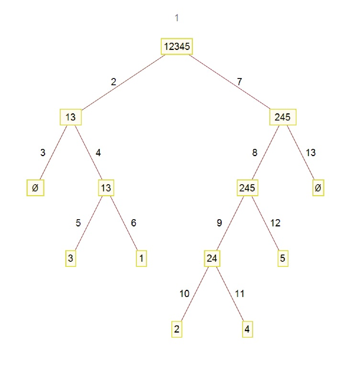
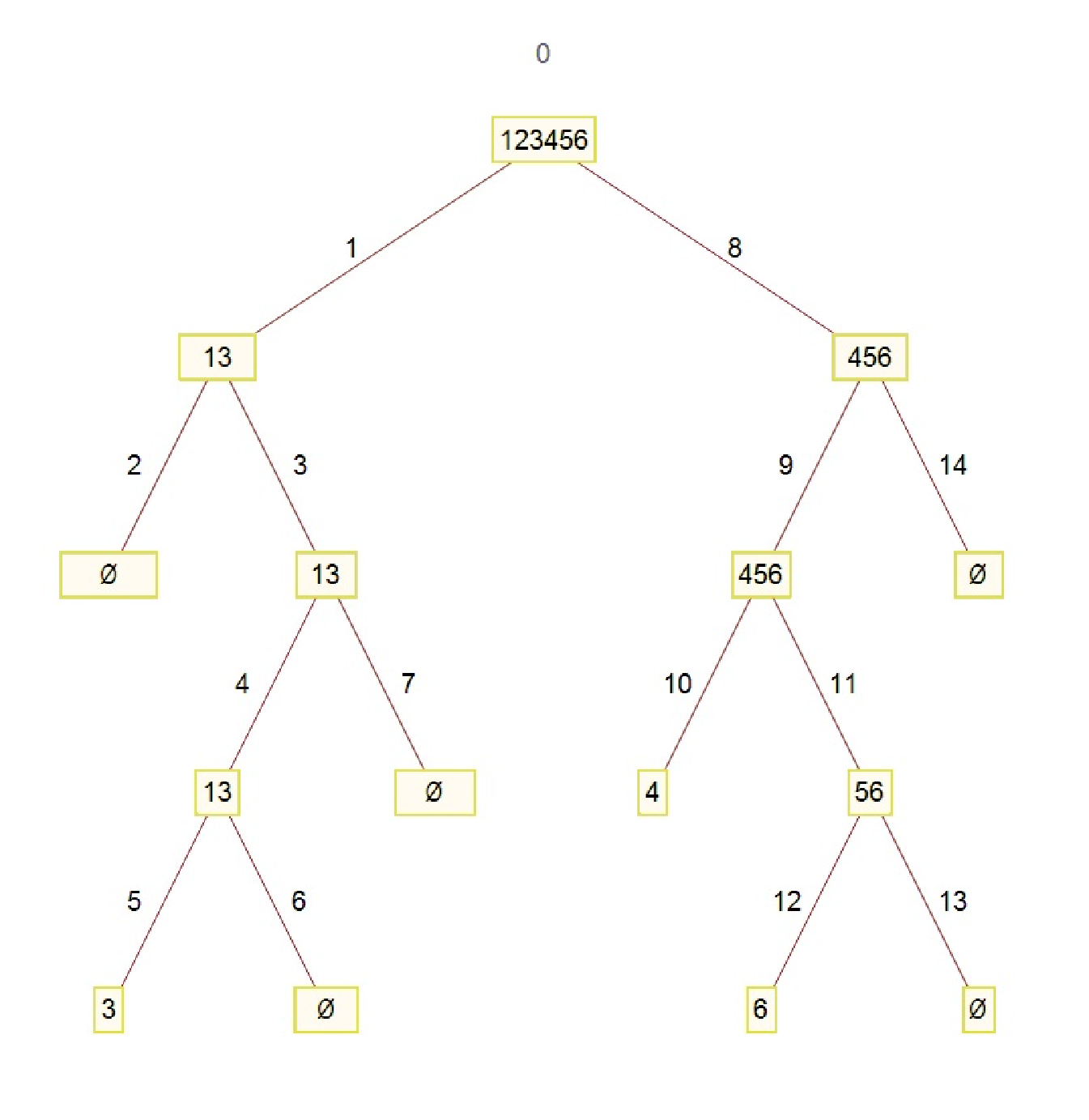
where the integer $k$ is initially $1$ , the list $L$ is initially $\{1,2,\ldots,n\}$ for simplicity’s sake, and $\operatorname{rbinom}(\cdot,1,0.5)$ is the built-in R unbiased random Bernoulli $\{0,1\}$ generator. Figure 1 exhibits a sample binary tree for $n=5$ . The first round of coin tosses yields $b=(0,1,0,1,1)$ , where $0=\operatorname{tail}$ and $1=\operatorname{head}$ , and thus $L_{1}=(1,3)$ , $L_{2}=(2,4,5)$ . On the left side, focusing on $L_{1}$ only, the next round of tosses yields $b^{\prime}=(1,1)$ and thus $L_{1}^{\prime}=\emptyset$ , $L_{2}^{\prime}=\{1,3\}$ . On the right side, focusing on $L_{2}$ only, the next round of tosses yields $b^{\prime\prime}=(0,0,0)$ and thus $L_{1}^{\prime\prime}=\{2,4,5\}$ , $L_{2}^{\prime\prime}=\emptyset$ . Also, focusing on $L_{1}^{\prime\prime}$ only, the next round of tosses yields $b^{\prime\prime\prime}=(0,0,1)$ and thus $L_{1}^{\prime\prime\prime}=\{2,4\}$ , $L_{2}^{\prime\prime\prime}=\{5\}$ . Termination occurs at the next level: any twig of the tree ceases to grow when its leaf contains $\leq 1$ items. The number of vertices (including empty vertices) is $13$ . We write $X_{5}=13$ . The labeled ordering of vertices is determined by watching $k$ increase, from $1$ to $13$ , as the algorithm progresses. Smaller values of $k$ occur on the left side because recursive splitting starts with $L_{1}$ , $L_{2}^{\prime}$ , … and thereafter continues with $L_{2}$ , $L_{1}^{\prime\prime}$ , $L_{1}^{\prime\prime\prime}$ , ….

Refer to caption — Figure 1: Strongly binary tree for conflict resolution.

The probability generating function for $X_{n}$ , given $n$ , is likewise recursive [3]:

\begin{array}[c]{ccc}f_{n}(z)=z2^{-n}{\displaystyle\sum\limits_{k=0}^{n}}\dbinom{n}{k}f_{k}(z)f_{n-k}(z),&&n\geq 2;\end{array}

f_{0}(z)=f_{1}(z)=z.

Note that $f_{n}(1)=1$ always. Differentiating with respect to $z$ :

f_{n}^{\prime}(z)=2^{-n}{\displaystyle\sum\limits_{k=0}^{n}}\dbinom{n}{k}f_{k}(z)f_{n-k}(z)+z2^{-n}{\displaystyle\sum\limits_{k=0}^{n}}\dbinom{n}{k}\left[f_{k}^{\prime}(z)f_{n-k}(z)+f_{k}(z)f_{n-k}^{\prime}(z)\right]

we have first moment

	$\displaystyle\mathbb{E}(X_{n})$	$\displaystyle=f_{n}^{\prime}(1)=1+2^{-n}{\displaystyle\sum\limits_{k=0}^{n}}\dbinom{n}{k}\left[f_{k}^{\prime}(1)+f_{n-k}^{\prime}(1)\right]$
		$\displaystyle=1+2^{1-n}{\displaystyle\sum\limits_{k=0}^{n}}\dbinom{n}{k}f_{k}^{\prime}(1),$

that is,

	$\displaystyle g_{n}$	$\displaystyle=1+2^{1-n}{\displaystyle\sum\limits_{k=0}^{n}}\dbinom{n}{k}g_{k}$
		$\displaystyle=\frac{1}{1-2^{1-n}}\left[1+2^{1-n}{\displaystyle\sum\limits_{k=0}^{n-1}}\dbinom{n}{k}g_{k}\right]$

where $g_{k}=f_{k}^{\prime}(1)$ and $g_{0}=g_{1}=1$ . Clearly $g_{2}=5$ and $g_{3}=23/3$ . Differentiating again:

	$\displaystyle f_{k}^{\prime\prime}(z)$	$\displaystyle=2^{1-n}{\displaystyle\sum\limits_{k=0}^{n}}\dbinom{n}{k}\left[f_{k}^{\prime}(z)f_{n-k}(z)+f_{k}(z)f_{n-k}^{\prime}(z)\right]$
		$\displaystyle+2^{-n}{\displaystyle\sum\limits_{k=0}^{n}}\dbinom{n}{k}\left[f_{k}^{\prime\prime}(z)f_{n-k}(z)+2f_{k}^{\prime}(z)f_{n-k}^{\prime}(z)+f_{k}(z)f_{n-k}^{\prime\prime}(z)\right]$

we have second factorial moment

	$\displaystyle\mathbb{E}(X_{n}(X_{n}-1))$	$\displaystyle=f_{n}^{\prime\prime}(1)$
		$\displaystyle=-2+2f_{n}^{\prime}(1)+2^{1-n}{\displaystyle\sum\limits_{k=0}^{n}}\dbinom{n}{k}f_{k}^{\prime}(1)f_{n-k}^{\prime}(1)+2^{1-n}{\displaystyle\sum\limits_{k=0}^{n}}\dbinom{n}{k}f_{k}^{\prime\prime}(1),$

that is,

	$\displaystyle h_{n}$	$\displaystyle=-2+2g_{n}+2^{1-n}{\displaystyle\sum\limits_{k=0}^{n}}\dbinom{n}{k}g_{k}g_{n-k}+2^{1-n}{\displaystyle\sum\limits_{k=0}^{n}}\dbinom{n}{k}h_{k}$
		$\displaystyle=\frac{1}{1-2^{1-n}}\left[-2+2g_{n}+2^{1-n}{\displaystyle\sum\limits_{k=0}^{n}}\dbinom{n}{k}g_{k}g_{n-k}+2^{1-n}{\displaystyle\sum\limits_{k=0}^{n-1}}\dbinom{n}{k}h_{k}\right]$

where $h_{k}=f_{k}^{\prime\prime}(1)$ and $h_{0}=h_{1}=0$ . Clearly $h_{2}=28$ and $h_{3}=548/9$ . Finally, we have variance

\mathbb{V}(X_{n})=h_{n}-g_{n}^{2}+g_{n}

which is $8$ when $n=2$ and $88/9$ when $n=3$ .

Such recursions are helpful for small $n$ , but give no asymptotic information as $n\rightarrow\infty$ . It can be proved that [4, 5]

	$\displaystyle\frac{\mathbb{E}(X_{n})}{n}$	$\displaystyle=\frac{2}{\ln(2)}+\delta_{1}\left(\frac{\ln(n)}{\ln(2)}\right)+o(1)$
		$\displaystyle\approx(2.8853900817...)+\,\delta_{1}\left(\log_{2}(n)\right),$

	$\displaystyle\frac{\mathbb{V}(X_{n})}{n}$	$\displaystyle=\frac{1}{\ln(2)}\left(1+8{\displaystyle\sum\limits_{k=1}^{\infty}}\frac{1}{(2^{k}+1)^{2}}\right)+\delta_{2}\left(\frac{\ln(n)}{\ln(2)}\right)+o(1)$
		$\displaystyle\approx(3.3834344923...)+\,\delta_{2}\left(\log_{2}(n)\right)$

where $\delta_{j}(x)$ is a periodic function of period $1$ with tiny amplitude and zero mean, for $j=1$ , $2$ . Functions like these appear throughout the analysis of algorithms. We shall not specify these here nor later, but merely indicate their presence when required. An infinite series representation of the mean for arbitrary $n$ is [6, 7]

\mathbb{E}(X_{n})=1+2{\displaystyle\sum\limits_{m=0}^{\infty}}2^{m}\left[1-\left(1-2^{-m}\right)^{n}-n2^{-m}\left(1-2^{-m}\right)^{n-1}\right].

Also, the constant $0.8458586230...$ (one-quarter of the variance as $n\rightarrow\infty$ ) appears in [8, 9, 10].

2 Leader Elections

Two parameters are examined in this section: height (length of the root-to-leaf path that gives the leader) and size (number of vertices in the associated weakly binary tree). We further discuss a variation of the election in which draws (involving exactly two competitors) constitute an additional way to stop the process.

2.1 Height

Consider the R program:

\begin{array}[c]{l}\text{{f $<$- function(L,k)}}\\ \text{{\lx@text@lbrace}}\\ \text{{\ \ if(NROW(L)$<$=1) \lx@text@lbrace}}\\ \text{{\ \ \ \ k}}\\ \text{{\ \ \lx@text@rbrace else \lx@text@lbrace}}\\ \text{{\ \ \ \ b $<$- rbinom(NROW(L),1,0.5)}}\\ \text{{\ \ \ \ L1 $<$- L[(1:NROW(L))*(1-b)]}}\\ \text{{\ \ \ \ k $<$- f(L1,k $<$- k+1)}}\\ \text{{\ \ \ \ if(NROW(L1)==0) \lx@text@lbrace}}\\ \text{{\ \ \ \ \ \ L2 $<$- L[(1:NROW(L))*b]}}\\ \text{{\ \ \ \ \ \ k $<$- f(L2,k)}}\\ \text{{\ \ \ \ \lx@text@rbrace}}\\ \text{{\ \ \lx@text@rbrace}}\\ \text{{\ \ k}}\\ \text{{\lx@text@rbrace}}\end{array}

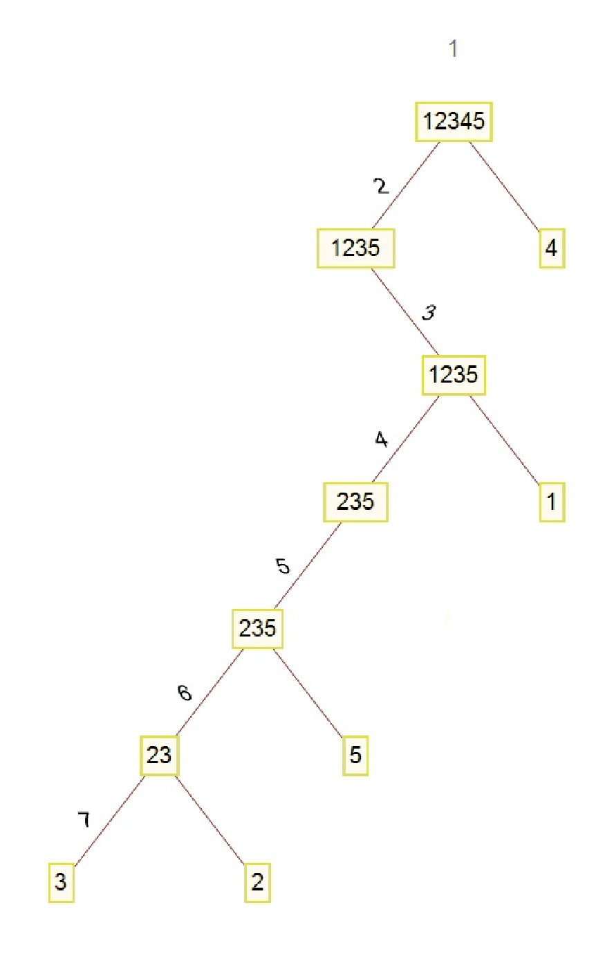
where the integer $k$ is initially $0$ (unlike before) and the list $L$ is initially $\{1,2,\ldots,n\}$ . Figure 2 exhibits a sample binary tree for $n=5$ . The first round of coin tosses yields $b=(0,0,0,1,0)$ , where $0=\operatorname{tail}$ and $1=\operatorname{head}$ , and thus $L_{1}=(1,2,3,5)$ , $L_{2}=(4)$ . Focusing on $L_{1}$ only, the next round of tosses yields $b^{\prime}=(1,1,1,1)$ and thus $L_{1}^{\prime}=\emptyset$ , $L_{2}^{\prime}=\{1,2,3,5\}$ . Note that we do not indicate nor count the empty vertex. Focusing on $L_{2}^{\prime}$ only, the next round of tosses yields $b^{\prime\prime}=(1,0,0,0)$ and thus $L_{1}^{\prime\prime}=\{2,3,5\}$ , $L_{2}^{\prime\prime}=\{1\}$ . Focusing on $L_{1}^{\prime\prime}$ only, the next round of tosses yields $b^{\prime\prime\prime}=(0,0,0)$ and thus $L_{1}^{\prime\prime\prime}=\{2,3,5\}$ , $L_{2}^{\prime\prime\prime}=\emptyset$ . Focusing on $L_{1}^{\prime\prime\prime}$ only, the next round of tosses yields $b^{\prime\prime\prime\prime}=(0,0,1)$ and thus $L_{1}^{\prime\prime\prime\prime}=\{2,3\}$ , $L_{2}^{\prime\prime\prime\prime}=\{5\}$ . Termination occurs at the next level: the leftmost twig of the tree contains exactly $1$ item. The height (number of steps separating the vertices labeled $1$ and $7$ ) is $6$ . We write $H_{5}=6$ .

The probability generating function for $H_{n}$ , given $n$ , is [11]:

\begin{array}[c]{ccc}f_{n}(z)=-z2^{-n}+z2^{-n}f_{n}(z)+z2^{-n}{\displaystyle\sum\limits_{k=0}^{n}}\dbinom{n}{k}f_{k}(z),&&n\geq 2;\end{array}

f_{0}(z)=f_{1}(z)=1.

Note that $f_{n}(1)=1$ always. Differentiating with respect to $z$ :

f_{n}^{\prime}(z)=-2^{-n}+2^{-n}f_{n}(z)+z2^{-n}f_{n}^{\prime}(z)+2^{-n}{\displaystyle\sum\limits_{k=0}^{n}}\dbinom{n}{k}f_{k}(z)+z2^{-n}{\displaystyle\sum\limits_{k=0}^{n}}\dbinom{n}{k}f_{k}^{\prime}(z)

we have first moment

	$\displaystyle\mathbb{E}(H_{n})$	$\displaystyle=f_{n}^{\prime}(1)=-2^{-n}+2^{-n}+2^{-n}f_{n}^{\prime}(1)+1+2^{-n}{\displaystyle\sum\limits_{k=0}^{n}}\dbinom{n}{k}f_{k}^{\prime}(1)$
		$\displaystyle=1+2^{-n}f_{n}^{\prime}(1)+2^{-n}{\displaystyle\sum\limits_{k=0}^{n}}\dbinom{n}{k}f_{k}^{\prime}(1),$

that is,

	$\displaystyle g_{n}$	$\displaystyle=1+2^{-n}g_{n}+2^{-n}{\displaystyle\sum\limits_{k=0}^{n}}\dbinom{n}{k}g_{k}$
		$\displaystyle=\frac{1}{1-2^{1-n}}\left[1+2^{-n}{\displaystyle\sum\limits_{k=0}^{n-1}}\dbinom{n}{k}g_{k}\right]$

where $g_{k}=f_{k}^{\prime}(1)$ and $g_{0}=g_{1}=0$ . Clearly $g_{2}=2$ and $g_{3}=7/3$ . Differentiating again:

f_{n}^{\prime\prime}(z)=2^{1-n}f_{n}^{\prime}(z)+z2^{-n}f_{n}^{\prime\prime}(z)+2^{1-n}{\displaystyle\sum\limits_{k=0}^{n}}\dbinom{n}{k}f_{k}^{\prime}(z)+z2^{-n}{\displaystyle\sum\limits_{k=0}^{n}}\dbinom{n}{k}f_{k}^{\prime\prime}(z)

we have second factorial moment

	$\displaystyle\mathbb{E}(H_{n}(H_{n}-1))$	$\displaystyle=f_{n}^{\prime\prime}(1)$
		$\displaystyle=-2+2f_{n}^{\prime}(1)+2^{-n}f_{n}^{\prime\prime}(1)+2^{-n}{\displaystyle\sum\limits_{k=0}^{n}}\dbinom{n}{k}f_{k}^{\prime\prime}(1),$

that is,

	$\displaystyle h_{n}$	$\displaystyle=-2+2g_{n}+2^{-n}h_{n}+2^{-n}{\displaystyle\sum\limits_{k=0}^{n}}\dbinom{n}{k}h_{k}$
		$\displaystyle=\frac{1}{1-2^{1-n}}\left[-2+2g_{n}+2^{-n}{\displaystyle\sum\limits_{k=0}^{n-1}}\dbinom{n}{k}h_{k}\right]$

where $h_{k}=f_{k}^{\prime\prime}(1)$ and $h_{0}=h_{1}=0$ . Clearly $h_{2}=4$ and $h_{3}=50/9$ . Finally, we have variance $\mathbb{V}(H_{n})$ which is $2$ when $n=2$ and $22/9$ when $n=3$ .

It can be proved that [12, 13, 14]

	$\displaystyle\mathbb{E}(H_{n})$	$\displaystyle=\frac{\ln(n)}{\ln(2)}+\frac{1}{2}+\delta_{3}\left(\frac{\ln(n)}{\ln(2)}\right)+o(1)$
		$\displaystyle\approx\log_{2}(n)+(0.5)+\delta_{3}(\log_{2}(n)),$

	$\displaystyle\mathbb{V}(H_{n})$	$\displaystyle=\frac{1}{12}+\frac{\pi^{2}}{6\ln(2)^{2}}-\frac{\gamma^{2}+2\gamma_{1}}{\ln(2)^{2}}+\varepsilon\left(\frac{\ln(n)}{\ln(2)}\right)+o(1)$
		$\displaystyle\approx(3.1166951643...)+\,\varepsilon\left(\log_{2}(n)\right)$

as $n\rightarrow\infty$ , where $\gamma_{1}$ is the first Stieltjes constant [15] and fluctuations provided by $\varepsilon(x)$ are symmetrical not about $0$ , but instead about [16]

{\displaystyle\int\limits_{0}^{1}}\varepsilon(x)dx=-\frac{1}{\ln(2)^{2}}{\displaystyle\sum\limits_{\begin{subarray}{c}k=-\infty\\ k\neq 0\end{subarray}}^{\infty}}\left|\zeta\left(1-\frac{2\pi ik}{\ln(2)}\right)\Gamma\left(1-\frac{2\pi ik}{\ln(2)}\right)\right|^{2}\approx-1.856\times 10^{-10}.

Needless to say, the evaluation of $\mathbb{V}(H_{n})$ is an impressive and difficult achievement.

2.2 Size

Consider the R program:

\begin{array}[c]{l}\text{{f $<$- function(L,k)}}\\ \text{{\lx@text@lbrace}}\\ \text{{\ \ if(NROW(L)$<$=1) \lx@text@lbrace}}\\ \text{{\ \ \ \ k}}\\ \text{{\ \ \lx@text@rbrace else \lx@text@lbrace}}\\ \text{{\ \ \ \ b $<$- rbinom(NROW(L),1,0.5)}}\\ \text{{\ \ \ \ L1 $<$- L[(1:NROW(L))*(1-b)]}}\\ \text{{\ \ \ \ L2 $<$- L[(1:NROW(L))*b]}}\\ \text{{\ \ \ \ k $<$- f(L1,k $<$- k+(NROW(L1)!=0)+(NROW(L2)!=0))}}\\ \text{{\ \ \ \ if(NROW(L1)==0) \lx@text@lbrace}}\\ \text{{\ \ \ \ \ \ k $<$- f(L2,k)}}\\ \text{{\ \ \ \ \lx@text@rbrace}}\\ \text{{\ \ \lx@text@rbrace}}\\ \text{{\ \ k}}\\ \text{{\lx@text@rbrace}}\end{array}

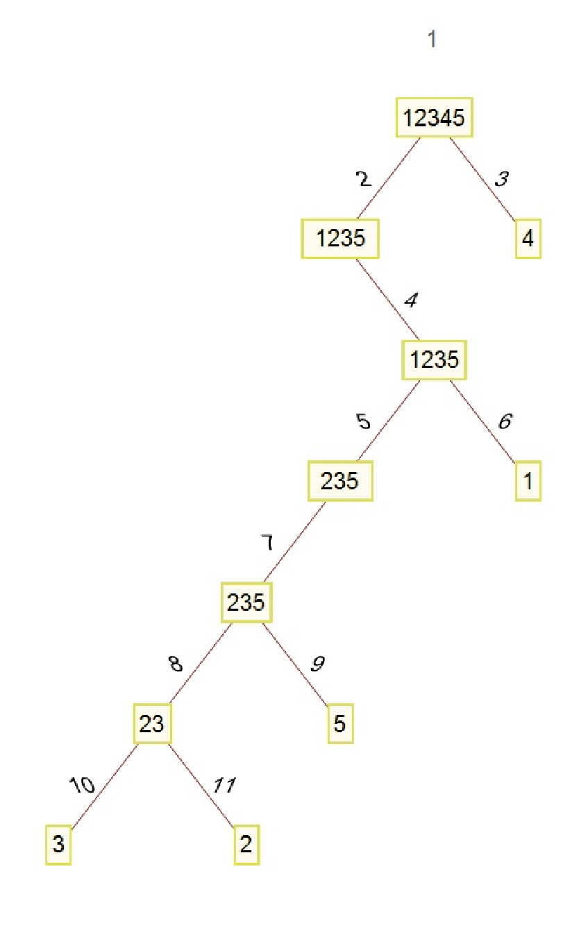
where the integer $k$ is initially $1$ and the list $L$ is initially $\{1,2,\ldots,n\}$ . Figure 3 is almost identical to Figure 2 – it contains the same binary tree for $n=5$ – but the labeling is different. The number of vertices (excluding empty vertices) is $11$ . We write $Y_{5}=11$ . The labeled ordering of vertices is determined by watching $k$ increase, from $1$ to $11$ , as the algorithm progresses. We sweep across the tree horizontally (in rows) rather than hierarchically. In particular, the command

\begin{array}[c]{l}\text{{k $<$- k+(NROW(L1)!=0)+(NROW(L2)!=0)}}\end{array}

increases $k$ by $2$ if both vertices are non-empty and by only $1$ if otherwise.

The probability generating function for $Y_{n}$ , given $n$ , is [11]:

\begin{array}[c]{ccc}f_{n}(z)=-z^{2}2^{-n}+\left(2z-z^{2}\right)2^{-n}f_{n}(z)+z^{2}2^{-n}{\displaystyle\sum\limits_{k=0}^{n}}\dbinom{n}{k}f_{k}(z),&&n\geq 2;\end{array}

\begin{array}[c]{ccc}f_{0}(z)=1,&&f_{1}(z)=z.\end{array}

Note that $f_{n}(1)=1$ always. Differentiating with respect to $z$ :

	$\displaystyle f_{n}^{\prime}(z)$	$\displaystyle=-z2^{1-n}+\left(1-z\right)2^{1-n}f_{n}(z)+\left(2z-z^{2}\right)2^{-n}f_{n}^{\prime}(z)$
		$\displaystyle+z2^{1-n}{\displaystyle\sum\limits_{k=0}^{n}}\dbinom{n}{k}f_{k}(z)+z^{2}2^{-n}{\displaystyle\sum\limits_{k=0}^{n}}\dbinom{n}{k}f_{k}^{\prime}(z)$

we have first moment

	$\displaystyle\mathbb{E}(Y_{n})$	$\displaystyle=f_{n}^{\prime}(1)=-2^{1-n}+0+2^{-n}f_{n}^{\prime}(1)+2+2^{-n}{\displaystyle\sum\limits_{k=0}^{n}}\dbinom{n}{k}f_{k}^{\prime}(1)$
		$\displaystyle=2-2^{1-n}+2^{-n}f_{n}^{\prime}(1)+2^{-n}{\displaystyle\sum\limits_{k=0}^{n}}\dbinom{n}{k}f_{k}^{\prime}(1),$

that is,

	$\displaystyle g_{n}$	$\displaystyle=\left(1-2^{1-n}\right)+1+2^{-n}g_{n}+2^{-n}{\displaystyle\sum\limits_{k=0}^{n}}\dbinom{n}{k}g_{k}$
		$\displaystyle=1+\frac{1}{1-2^{1-n}}\left[1+2^{-n}{\displaystyle\sum\limits_{k=0}^{n-1}}\dbinom{n}{k}g_{k}\right]$

where $g_{k}=f_{k}^{\prime}(1)$ and $g_{0}=0$ , $g_{1}=1$ . Clearly $g_{2}=4$ and $g_{3}=29/6$ . Differentiating again:

	$\displaystyle f_{n}^{\prime\prime}(z)$	$\displaystyle=-2^{1-n}-2^{1-n}f_{n}(z)+(1-z)2^{2-n}f_{n}^{\prime}(z)+\left(2z-z^{2}\right)2^{-n}f_{n}^{\prime\prime}(z)$
		$\displaystyle+2^{1-n}{\displaystyle\sum\limits_{k=0}^{n}}\dbinom{n}{k}f_{k}(z)+z2^{2-n}{\displaystyle\sum\limits_{k=0}^{n}}\dbinom{n}{k}f_{k}^{\prime}(z)+z^{2}2^{-n}{\displaystyle\sum\limits_{k=0}^{n}}\dbinom{n}{k}f_{k}^{\prime\prime}(z)$

we have second factorial moment

	$\displaystyle\mathbb{E}(Y_{n}(Y_{n}-1))$	$\displaystyle=f_{n}^{\prime\prime}(1)$
		$\displaystyle=-2^{2-n}+0+2^{-n}f_{n}^{\prime\prime}(1)+2+2^{2-n}{\displaystyle\sum\limits_{k=0}^{n}}\dbinom{n}{k}f_{k}^{\prime}(1)+2^{-n}{\displaystyle\sum\limits_{k=0}^{n}}\dbinom{n}{k}f_{k}^{\prime\prime}(1),$

that is,

	$\displaystyle h_{n}$	$\displaystyle=2\left(1-2^{1-n}\right)+2^{-n}h_{n}+2^{2-n}{\displaystyle\sum\limits_{k=0}^{n}}\dbinom{n}{k}g_{k}+2^{-n}{\displaystyle\sum\limits_{k=0}^{n}}\dbinom{n}{k}h_{k}$
		$\displaystyle=2+\frac{1}{1-2^{1-n}}\left[2^{2-n}{\displaystyle\sum\limits_{k=0}^{n}}\dbinom{n}{k}g_{k}+2^{-n}{\displaystyle\sum\limits_{k=0}^{n-1}}\dbinom{n}{k}h_{k}\right]$

where $h_{k}=f_{k}^{\prime\prime}(1)$ and $h_{0}=h_{1}=0$ . Clearly $h_{2}=14$ and $h_{3}=200/9$ . Finally, we have variance $\mathbb{V}(Y_{n})$ which is $2$ when $n=2$ and $133/36$ when $n=3$ .

It can be proved that [11]

	$\displaystyle\mathbb{E}(Y_{n})$	$\displaystyle=\frac{2\ln(n)}{\ln(2)}+\left(2-\frac{\ln(\pi)-\gamma}{\ln(2)}\right)+\delta_{4}\left(\frac{\ln(n)}{\ln(2)}\right)+o(1)$
		$\displaystyle\approx 2\log_{2}(n)+(1.1812500478...)+\delta_{4}(\log_{2}(n))$

as $n\rightarrow\infty$ , but a comparable asymptotic expression for $\mathbb{V}(Y_{n})$ remains unknown.

We wonder about the cross-covariance of $H_{n}$ and $Y_{n}$ , whose calculation would require a bivariate generating function.

2.3 Draws

Let us alter the rules so that a draw between two persons is allowed (if precisely two persons are left, then they both are declared leaders). The third line of the two preceding R programs is simply replaced by

\begin{array}[c]{l}\text{{if(NROW(L)$<$=2) \lx@text@lbrace}}\end{array}

and the initial conditions of the two preceding $\{g_{n},h_{n}\}$ recurrences are also changed. For height, we now have $g_{0}=g_{1}=g_{2}=0$ (implying $g_{3}=4/3)$ and $h_{0}=h_{1}=h_{2}=0$ (implying $h_{3}=8/9$ ); thus

	$\displaystyle\mathbb{E}(\tilde{H}_{n})$	$\displaystyle=\frac{\ln(n)}{\ln(2)}+\left(\frac{1}{2}-\frac{\pi^{2}}{12\ln(2)}\right)+\delta_{5}\left(\frac{\ln(n)}{\ln(2)}\right)+o(1)$
		$\displaystyle\approx\log_{2}(n)-(0.6865691104...)+\delta_{5}(\log_{2}(n)).$

For size, we now have $g_{0}=0$ , $g_{1}=g_{2}=1$ (implying $g_{3}=10/3)$ and $h_{0}=h_{1}=h_{2}=0$ (implying $h_{3}=74/9$ ); thus

	$\displaystyle\mathbb{E}(\tilde{Y}_{n})$	$\displaystyle=\frac{2\ln(n)}{\ln(2)}+\left(2-\frac{\ln(\pi)-\gamma+\frac{\pi^{2}}{8}}{\ln(2)}\right)+\delta_{6}\left(\frac{\ln(n)}{\ln(2)}\right)+o(1)$
		$\displaystyle\approx 2\log_{2}(n)-(0.5986036178...)+\delta_{6}(\log_{2}(n)).$

It would seem that the fraction $\pi^{2}/16$ given within the formula for $\mathbb{E}(\tilde{Y}_{n})$ in [11] is incorrect and should be $\pi^{2}/8$ instead.

3 Coin Tosses

Before moving on to more complicated examples, it may be worthwhile to contemplate the most elementary recursive program imaginable:

\begin{array}[c]{l}\text{{f $<$- function(L,k)}}\\ \text{{\lx@text@lbrace}}\\ \text{{\ \ if(NROW(L)==0) \lx@text@lbrace}}\\ \text{{\ \ \ \ k}}\\ \text{{\ \ \lx@text@rbrace else \lx@text@lbrace}}\\ \text{{\ \ \ \ b $<$- rbinom(NROW(L),1,0.5)}}\\ \text{{\ \ \ \ L1 $<$- L[(1:NROW(L))*(1-b)]}}\\ \text{{\ \ \ \ k $<$- f(L1,k $<$- k+1)}}\\ \text{{\ \ \lx@text@rbrace}}\\ \text{{\ \ k}}\\ \text{{\lx@text@rbrace}}\end{array}

mentioned at the end of [17], where $k$ is initially $0$ . Note that the third line here is

\begin{array}[c]{l}\text{{if(NROW(L)$<$=0) \lx@text@lbrace}}\end{array}

unlike what we have seen before. People iteratively toss all coins which show tails until only heads are visible. Omitting details, it follows that the procedural height has generating function

\begin{array}[c]{ccc}f_{n}(z)=z2^{-n}{\displaystyle\sum\limits_{k=0}^{n}}\dbinom{n}{k}f_{k}(z),&&n\geq 1;\end{array}

f_{0}(z)=1

therefore

g_{n}=1+2^{-n}{\displaystyle\sum\limits_{k=0}^{n}}\dbinom{n}{k}g_{k}=\frac{1}{1-2^{-n}}\left[1+2^{-n}{\displaystyle\sum\limits_{k=0}^{n-1}}\dbinom{n}{k}g_{k}\right],

h_{n}=-2+2g_{n}+2^{-n}{\displaystyle\sum\limits_{k=0}^{n}}\dbinom{n}{k}h_{k}=\frac{1}{1-2^{-n}}\left[-2+2g_{n}+2^{-n}{\displaystyle\sum\limits_{k=0}^{n-1}}\dbinom{n}{k}h_{k}\right]

where $g_{0}=0$ (implying $g_{1}=2$ , $g_{2}=8/3$ , $g_{3}=22/7)$ and $h_{0}=0$ (implying $h_{1}=4$ , $h_{2}=64/9$ , $h_{3}=1420/147$ ). From this [18]

	$\displaystyle\mathbb{E}(\hat{H}_{n})$	$\displaystyle=\frac{\ln(n)}{\ln(2)}+\left(\frac{1}{2}+\frac{\gamma}{\ln(2)}\right)+\delta_{7}\left(\frac{\ln(n)}{\ln(2)}\right)+o(1)$
		$\displaystyle\approx\log_{2}(n)+(1.3327461772...)+\delta_{7}(\log_{2}(n)),$

	$\displaystyle\mathbb{V}(\hat{H}_{n})$	$\displaystyle=\left(\frac{1}{12}+\frac{\pi^{2}}{6\ln(2)^{2}}\right)+\delta_{8}\left(\frac{\ln(n)}{\ln(2)}\right)+o(1)$
		$\displaystyle\approx(3.5070480758...)+\,\delta_{8}\left(\log_{2}(n)\right)$

as $n\rightarrow\infty$ .

4 Finding the Maximum

Consider the R program:

\begin{array}[c]{l}\text{{f $<$- function(L,k,r)}}\\ \text{{\lx@text@lbrace}}\\ \text{{\ \ if(NROW(L)==0) \lx@text@lbrace}}\\ \text{{\ \ \ \ c(k,r)}}\\ \text{{\ \ \lx@text@rbrace else if(NROW(L)==1) \lx@text@lbrace}}\\ \text{{\ \ \ \ c(k,r $<$- max(L,r))}}\\ \text{{\ \ \lx@text@rbrace else \lx@text@lbrace}}\\ \text{{\ \ \ \ b $<$- rbinom(NROW(L),1,0.5)}}\\ \text{{\ \ \ \ L0 $<$- L[(1:NROW(L))*b]}}\\ \text{{\ \ \ \ L1 $<$- L[(1:NROW(L))*(1-b)]}}\\ \text{{\ \ \ \ V $<$- f(L1,k $<$- k+1,r)}}\\ \text{{\ \ \ \ k $<$- V[1]; r $<$- V[2]}}\\ \text{{\ \ \ \ L2 $<$- L0[L0$>$r]}}\\ \text{{\ \ \ \ V $<$- f(L2,k $<$- k+1,r)}}\\ \text{{\ \ \ \ k $<$- V[1]; r $<$- V[2]}}\\ \text{{\ \ \lx@text@rbrace}}\\ \text{{\ \ c(k,r)}}\\ \text{{\lx@text@rbrace}}\end{array}

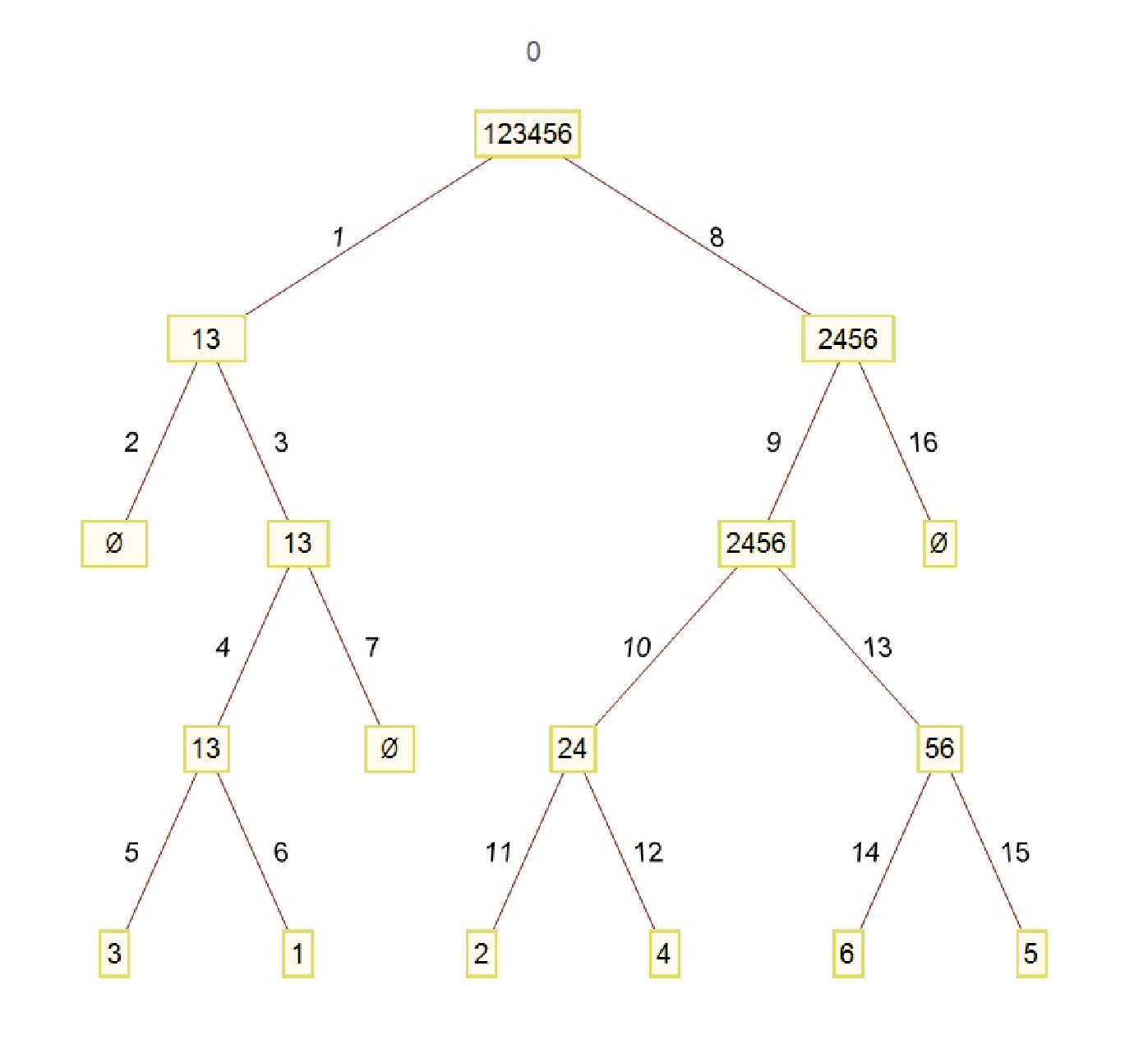
where the integer $k$ is initially $0$ and the list $L$ is initially $\{1,2,\ldots,n\}$ . We find a comparison of a conflict resolution tree in Figure 4 and its corresponding maximum-finding tree in Figure 5 to be helpful. Note that the vertex count for the latter is only $14$ , which is less than the vertex count of $16$ determined for the former. The discrepancy arises because, at the instant the $5^{\text{th}}$ vertex $3$ becomes the leader and $r$ consequently increases from $0$ to $3$ , both the $6^{\text{th}}$ vertex $1$ becomes empty and the $8^{\text{th}}$ & $9^{\text{th}}$ vertices $2456$ are reduced to $456$ . It follows that the $10^{\text{th}}$ vertex $24$ is reduced to $4$ , which cannot have any descendants, eliminating two twigs. Also, $r$ increases from $3$ to $4$ and, subsequently, from $4$ to $6$ ; while the penultimate vertex becomes empty, this does not further alter the count. We write $X_{6}=14$ .

The probability generating function for $X_{n}$ , given $n$ , is [19, 20, 21, 22]:

\begin{array}[c]{ccc}f_{n}(z)=z^{2}2^{-n}f_{n}(z)+z2^{-n}{\displaystyle\sum\limits_{k=1}^{n}}f_{n-k}(z){\displaystyle\sum\limits_{j=1}^{k}}\dbinom{k-1}{j-1}f_{j}(z),&&n\geq 2;\end{array}

f_{0}(z)=f_{1}(z)=z.

Note that $f_{n}(1)=1$ always. When differentiating with respect to $z$ :

	$\displaystyle f_{n}^{\prime}(z)$	$\displaystyle=z2^{1-n}f_{n}(z)+z^{2}2^{-n}f_{n}^{\prime}(z)+2^{-n}{\displaystyle\sum\limits_{k=1}^{n}}f_{n-k}(z){\displaystyle\sum\limits_{j=1}^{k}}\dbinom{k-1}{j-1}f_{j}(z)$
		$\displaystyle+z2^{-n}{\displaystyle\sum\limits_{k=1}^{n}}f_{n-k}^{\prime}(z){\displaystyle\sum\limits_{j=1}^{k}}\dbinom{k-1}{j-1}f_{j}(z)+z2^{-n}{\displaystyle\sum\limits_{j=1}^{n}}f_{j}^{\prime}(z){\displaystyle\sum\limits_{k=j}^{n}}\dbinom{k-1}{j-1}f_{n-k}(z)$

we make use of the identity

{\displaystyle\sum\limits_{k=1}^{n}}{\displaystyle\sum\limits_{j=1}^{k}}a_{kj}={\displaystyle\sum\limits_{j=1}^{n}}{\displaystyle\sum\limits_{k=j}^{n}}a_{kj}.

From this follows the first moment:

	$\displaystyle\mathbb{E}(X_{n})$	$\displaystyle=f_{n}^{\prime}(1)=2^{1-n}+2^{-n}f_{n}^{\prime}(1)+2^{-n}\left(-1+2^{n}\right)+2^{-n}{\displaystyle\sum\limits_{k=1}^{n}}2^{-1+k}f_{n-k}^{\prime}(1)+2^{-n}{\displaystyle\sum\limits_{j=1}^{n}}\dbinom{n}{j}f_{j}^{\prime}(1)$
		$\displaystyle=1-2^{-n}+2^{1-n}+2^{-n}f_{n}^{\prime}(1)+{\displaystyle\sum\limits_{k=1}^{n}}2^{-1-n+k}f_{n-k}^{\prime}(1)+2^{-n}{\displaystyle\sum\limits_{j=0}^{n-1}}\dbinom{n}{j}f_{j}^{\prime}(1)-2^{-n}+2^{-n}f_{n}^{\prime}(1)$
		$\displaystyle=1+2^{1-n}f_{n}^{\prime}(1)+{\displaystyle\sum\limits_{i=0}^{n-1}}2^{-i-1}f_{i}^{\prime}(1)+2^{-n}{\displaystyle\sum\limits_{j=0}^{n-1}}\dbinom{n}{j}f_{j}^{\prime}(1)$

setting $i=n-k$ , hence $i+1=1+n-k$ and $0\leq i\leq n-1$ when $1\leq k\leq n$ . That is,

	$\displaystyle g_{n}$	$\displaystyle=1+2^{1-n}g_{n}+{\displaystyle\sum\limits_{i=0}^{n-1}}\left[2^{-n}\dbinom{n}{i}+2^{-i-1}\right]g_{i}$
		$\displaystyle=\frac{1}{1-2^{1-n}}\left\{1+{\displaystyle\sum\limits_{i=0}^{n-1}}\left[2^{-n}\dbinom{n}{i}+2^{-i-1}\right]g_{i}\right\}$

where $g_{i}=f_{i}^{\prime}(1)$ and $g_{0}=g_{1}=1$ . Clearly $g_{2}=5$ and $g_{3}=19/3$ . Differentiating again:

	$\displaystyle f_{n}^{\prime\prime}(z)$	$\displaystyle=2^{1-n}f_{n}(z)+z2^{2-n}f_{n}^{\prime}(z)+z^{2}2^{-n}f_{n}^{\prime\prime}(z)$
		$\displaystyle+2^{1-n}{\displaystyle\sum\limits_{k=1}^{n}}f_{n-k}^{\prime}(z){\displaystyle\sum\limits_{j=1}^{k}}\dbinom{k-1}{j-1}f_{j}(z)+2^{1-n}{\displaystyle\sum\limits_{j=1}^{n}}f_{j}^{\prime}(z){\displaystyle\sum\limits_{k=j}^{n}}\dbinom{k-1}{j-1}f_{n-k}(z)$
		$\displaystyle+z2^{-n}{\displaystyle\sum\limits_{k=1}^{n}}f_{n-k}^{\prime\prime}(z){\displaystyle\sum\limits_{j=1}^{k}}\dbinom{k-1}{j-1}f_{j}(z)+z2^{-n}{\displaystyle\sum\limits_{j=1}^{n}}f_{j}^{\prime\prime}(z){\displaystyle\sum\limits_{k=j}^{n}}\dbinom{k-1}{j-1}f_{n-k}(z)$
		$\displaystyle+z2^{1-n}{\displaystyle\sum\limits_{k=1}^{n}}f_{n-k}^{\prime}(z){\displaystyle\sum\limits_{j=1}^{k}}\dbinom{k-1}{j-1}f_{j}^{\prime}(z)$

and employing

	$\displaystyle 2^{-n}{\displaystyle\sum\limits_{k=1}^{n}}2^{-1+k}f_{n-k}^{\prime}(1)+2^{-n}{\displaystyle\sum\limits_{j=1}^{n}}\dbinom{n}{j}f_{j}^{\prime}(1)$	$\displaystyle=f_{n}^{\prime}(1)-\left[1-2^{-n}+2^{1-n}+2^{-n}f_{n}^{\prime}(1)\right]$
		$\displaystyle=-1-2^{-n}+\left(1-2^{-n}\right)f_{n}^{\prime}(1),$

we have second factorial moment

	$\displaystyle\mathbb{E}(X_{n}(X_{n}-1))$	$\displaystyle=f_{n}^{\prime\prime}(1)$
		$\displaystyle=2^{1-n}+2^{2-n}f_{n}^{\prime}(1)+2^{-n}f_{n}^{\prime\prime}(1)+2\left[-1-2^{-n}+\left(1-2^{-n}\right)f_{n}^{\prime}(1)\right]$
		$\displaystyle+{\displaystyle\sum\limits_{i=0}^{n-1}}2^{-i-1}f_{i}^{\prime\prime}(1)+{\displaystyle\sum\limits_{i=0}^{n-1}}2^{-n}\dbinom{n}{i}f_{i}^{\prime\prime}(1)+2^{-n}f_{n}^{\prime\prime}(1)+2^{1-n}{\displaystyle\sum\limits_{k=1}^{n}}f_{n-k}^{\prime}(1){\displaystyle\sum\limits_{j=1}^{k}}\dbinom{k-1}{j-1}f_{j}^{\prime}(1)$

that is,

	$\displaystyle h_{n}$	$\displaystyle=-2+2\left(1+2^{-n}\right)g_{n}+2^{1-n}h_{n}+{\displaystyle\sum\limits_{i=0}^{n-1}}\left[2^{-n}\dbinom{n}{i}+2^{-i-1}\right]h_{i}+2^{1-n}{\displaystyle\sum\limits_{k=1}^{n}}g_{n-k}{\displaystyle\sum\limits_{j=1}^{k}}\dbinom{k-1}{j-1}g_{j}$
		$\displaystyle=\frac{1}{1-2^{1-n}}\left\{-2+2\left(1+2^{-n}\right)g_{n}+{\displaystyle\sum\limits_{i=0}^{n-1}}\left[2^{-n}\dbinom{n}{i}+2^{-i-1}\right]h_{i}+2^{1-n}{\displaystyle\sum\limits_{k=1}^{n}}{\displaystyle\sum\limits_{j=1}^{k}}\dbinom{k-1}{j-1}g_{j}g_{n-k}\right\}$

where $h_{k}=f_{k}^{\prime\prime}(1)$ and $h_{0}=h_{1}=0$ . Clearly $h_{2}=28$ and $h_{3}=400/9$ . Finally, we have variance $\mathbb{V}(X_{n})$ which is $8$ when $n=2$ and $32/3$ when $n=3$ .

It can be proved that [21, 22]

	$\displaystyle\mathbb{E}(X_{n})$	$\displaystyle=\frac{\pi^{2}}{3\ln(2)}\ln(n)+\delta_{9}\left(\frac{\ln(n)}{\ln(2)}\right)+o(1)$
		$\displaystyle\approx(4.7462764416...)\ln(n)+\delta_{9}(\log_{2}(n)),$

	$\displaystyle\mathbb{V}(X_{n})$	$\displaystyle=\frac{1}{\ln(2)}\left(\pi^{2}-2-\frac{\pi^{4}}{9}+{\displaystyle\sum\limits_{i=0}^{\infty}}2^{-i-1}h_{i}\right)\ln(n)+O(1)$
		$\displaystyle\approx(11.7013270183...)\ln(n)+\,O(1)$

as $n\rightarrow\infty$ . Although the leading coefficient for $\mathbb{V}(X_{n})$ is recursive (involving $h_{i}$ ), the series converges rapidly enough for numerical purposes.

Shiau & Yang [23] mentioned a slight revision of the preceding algorithm, but details are unclear. To discuss this, we write $Y_{n}$ for the vertex count rather than $X_{n}$ . In particular, they gave $\mathbb{E}(Y_{2})=9/2$ . We hypothesize that, in the maximization R code given earlier, replacing the line

\begin{array}[c]{l}\text{{V $<$- f(L2,k $<$- k+1,r)}}\end{array}

by the two lines:

\begin{array}[c]{l}\text{{if(NROW(L1)$>$=1) k $<$- k+1}}\\ \text{{V $<$- f(L2,k,r)}}\end{array}

might duplicate the revised procedure. This has the effect of eliminating the $2^{\text{nd}}$ vertex $\emptyset$ in Figure 5 (because the $3^{\text{rd}}$ vertex $13$ will be assigned the same label $2$ ). It makes sense to remove left-empty vertices from consideration for efficiency (as would removing right-empty vertices, or both). Simulation suggests that, indeed, the average vertex count is $9/2$ when $n=2$ . We have not further pursued this issue.

Chen & Hwang [22] analyzed a different algorithm, based on leader elections, that starts afresh with every iteration. It is not surprising that vertex counts are $O\left(\ln(n)^{2}\right)$ for the mean and $O\left(\ln(n)^{3}\right)$ for the variance, notably slower than the conflict resolution-based approach.

5 Sorting a List

Consider the R programs:

\begin{array}[c]{l}\text{{phi $<$- function(L,k,s)}}\\ \text{{\lx@text@lbrace}}\\ \text{{\ \ if(NROW(L)==0) \lx@text@lbrace}}\\ \text{{\ \ \ \ c(k,s)}}\\ \text{{\ \ \lx@text@rbrace else if(NROW(L)==1) \lx@text@lbrace}}\\ \text{{\ \ \ \ c(k,s $<$- L[1])}}\\ \text{{\ \ \lx@text@rbrace else \lx@text@lbrace}}\\ \text{{\ \ \ \ b $<$- rbinom(NROW(L),1,0.5)}}\\ \text{{\ \ \ \ L1 $<$- L[(1:NROW(L))*(1-b)]}}\\ \text{{\ \ \ \ V $<$- phi(L1,k $<$- k+1,s)}}\\ \text{{\ \ \ \ k $<$- V[1]; s $<$- V[2]}}\\ \text{{\ \ \ \ if(NROW(L1)==0) \lx@text@lbrace}}\\ \text{{\ \ \ \ \ \ L2 $<$- L[(1:NROW(L))*b]}}\\ \text{{\ \ \ \ \ \ V $<$- phi(L2,k,s)}}\\ \text{{\ \ \ \ \ \ k $<$- V[1]; s $<$- V[2]}}\\ \text{{\ \ \ \ \lx@text@rbrace}}\\ \text{{\ \ \lx@text@rbrace}}\\ \text{{\ \ c(k,s)}}\\ \text{{\lx@text@rbrace}}\end{array}

and

\begin{array}[c]{l}\text{{psi $<$- function(L)}}\\ \text{{\lx@text@lbrace}}\\ \text{{\ \ if(NROW(L)$<$=1) \lx@text@lbrace}}\\ \text{{\ \ \ \ k $<$- 1}}\\ \text{{\ \ \lx@text@rbrace else \lx@text@lbrace}}\\ \text{{\ \ \ \ V $<$- phi(L,0,0)}}\\ \text{{\ \ \ \ k $<$- 1+V[1]; s $<$- V[2]}}\\ \text{{\ \ \ \ k $<$- k+psi(L[L$<$s])+psi(L[L$>$s])}}\\ \text{{\ \ \lx@text@rbrace}}\\ \text{{\ \ k}}\\ \text{{\lx@text@rbrace}}\end{array}

where the list $L$ is initially $\{1,2,\ldots,n\}$ . The function $\varphi$ accomplishes the same task as $f$ does in Section 2.1, but additionally monitors the leader $s$ , whose value acts as a pivot for the recursive splitting of $L$ within the function $\psi$ . Define $K_{n}$ to be the “height” of the sorting algorithm captured by $\psi$ , that is, the sum (over all elections) of required time lengths plus one.

The probability generating function for $K_{n}$ , given $n$ , is

\begin{array}[c]{ccc}\psi_{n}(z)=\dfrac{zf_{n}(z)}{n}{\displaystyle\sum\limits_{k=0}^{n-1}}\psi_{k}(z)\psi_{n-k-1}(z),&&n\geq 2;\end{array}

\psi_{0}(z)=\psi_{1}(z)=z

where $f_{n}$ is exactly as in Section 2.1. Note that $\psi_{n}(1)=1$ always. Differentiating with respect to $z$ :

\psi_{n}^{\prime}(z)=\dfrac{f_{n}(z)+zf_{n}^{\prime}(z)}{n}{\displaystyle\sum\limits_{k=0}^{n-1}}\psi_{k}(z)\psi_{n-k-1}(z)+\dfrac{zf_{n}(z)}{n}{\displaystyle\sum\limits_{k=0}^{n-1}}\left[\psi_{k}^{\prime}(z)\psi_{n-k-1}(z)+\psi_{k}(z)\psi_{n-k-1}^{\prime}(z)\right]

we have first moment

	$\displaystyle\mathbb{E}(K_{n})$	$\displaystyle=\psi_{n}^{\prime}(1)=\dfrac{1+f_{n}^{\prime}(1)}{n}{\displaystyle\sum\limits_{k=0}^{n-1}}1+\dfrac{1}{n}{\displaystyle\sum\limits_{k=0}^{n-1}}\left[\psi_{k}^{\prime}(1)+\psi_{n-k-1}^{\prime}(1)\right]$
		$\displaystyle=1+f_{n}^{\prime}(1)+\dfrac{2}{n}{\displaystyle\sum\limits_{k=0}^{n-1}}\psi_{k}^{\prime}(1),$

that is [24, 25],

\xi_{n}=1+g_{n}+\dfrac{2}{n}{\displaystyle\sum\limits_{k=0}^{n-1}}\xi_{k}

where $g_{k}=f_{k}^{\prime}(1)$ , $\xi_{k}=\psi_{k}^{\prime}(1)$ and $\xi_{0}=\xi_{1}=1$ . Clearly $\xi_{2}=5$ and $\xi_{3}=8$ . Differentiating again:

	$\displaystyle\psi_{n}^{\prime\prime}(z)$	$\displaystyle=\dfrac{2f_{n}^{\prime}(z)+zf_{n}^{\prime\prime}(z)}{n}{\displaystyle\sum\limits_{k=0}^{n}}\psi_{k}(z)\psi_{n-k-1}(z)$
		$\displaystyle+\dfrac{2f_{n}(z)+2zf_{n}^{\prime}(z)}{n}{\displaystyle\sum\limits_{k=0}^{n-1}}\left[\psi_{k}^{\prime}(z)\psi_{n-k-1}(z)+\psi_{k}(z)\psi_{n-k-1}^{\prime}(z)\right]$
		$\displaystyle+\dfrac{zf_{n}(z)}{n}{\displaystyle\sum\limits_{k=0}^{n-1}}\left[\psi_{k}^{\prime\prime}(z)\psi_{n-k-1}(z)+2\psi_{k}^{\prime}(z)\psi_{n-k-1}^{\prime}(z)+\psi_{k}(z)\psi_{n-k-1}^{\prime\prime}(z)\right]$

we have second factorial moment

	$\displaystyle\mathbb{E}(K_{n}(K_{n}-1))$	$\displaystyle=\psi_{n}^{\prime\prime}(1)$
		$\displaystyle=\dfrac{2f_{n}^{\prime}(1)+f_{n}^{\prime\prime}(1)}{n}{\displaystyle\sum\limits_{k=0}^{n}}1+\dfrac{2+2f_{n}^{\prime}(1)}{n}{\displaystyle\sum\limits_{k=0}^{n-1}}\left[\psi_{k}^{\prime}(1)+\psi_{n-k-1}^{\prime}(1)\right]$
		$\displaystyle+\dfrac{1}{n}{\displaystyle\sum\limits_{k=0}^{n-1}}\left[\psi_{k}^{\prime\prime}(1)+2\psi_{k}^{\prime}(1)\psi_{n-k-1}^{\prime}(1)+\psi_{n-k-1}^{\prime\prime}(1)\right]$
		$\displaystyle=2f_{n}^{\prime}(1)+f_{n}^{\prime\prime}(1)+\dfrac{4+4f_{n}^{\prime}(1)}{n}{\displaystyle\sum\limits_{k=0}^{n-1}}\psi_{k}^{\prime}(1)+\dfrac{2}{n}{\displaystyle\sum\limits_{k=0}^{n-1}}\left[\psi_{k}^{\prime\prime}(1)+\psi_{k}^{\prime}(1)\psi_{n-k-1}^{\prime}(1)\right]$

that is,

\eta_{n}=2g_{n}+h_{n}-2\left(1+g_{n}\right)\left(1+g_{n}-\xi_{n}\right)+\dfrac{2}{n}{\displaystyle\sum\limits_{k=0}^{n-1}}\left(\eta_{k}+\xi_{k}\xi_{n-k-1}\right)

where $h_{k}=f_{k}^{\prime\prime}(1)$ , $\eta_{k}=\psi_{k}^{\prime\prime}(1)$ and $\eta_{0}=\eta_{1}=0$ . As far as is known, this recurrence has not previously appeared in the literature. Clearly $\eta_{2}=22$ and $\eta_{3}=190/3$ . Finally, we have variance $\mathbb{V}(K_{n})$ which is $2$ when $n=2$ and $22/3$ when $n=3$ . It can be proved that [25]

	$\displaystyle\frac{\mathbb{E}(K_{n})}{n}$	$\displaystyle=\frac{8}{3}+2{\displaystyle\sum\limits_{\ell=3}^{\infty}}\frac{g_{\ell}-g_{\ell-1}}{\ell+1}+o(1)$
		$\displaystyle\approx 3.5455178132...\approx 8/3+2(0.4394255733...)$

as $n\rightarrow\infty$ , but a comparable limit for $\mathbb{V}(K_{n})$ remains unknown.

Grabner & Prodinger [25] examined a different sorting algorithm [23, 26], based on the preceding maximization strategy, that is somewhat more involved yet does not perform quite as well:

	$\displaystyle\frac{\mathbb{E}(\tilde{K}_{n})}{n}$	$\displaystyle=\frac{13}{6}+{\displaystyle\sum\limits_{\ell=3}^{\infty}}\frac{g_{\ell}-g_{\ell-1}}{\ell+1}+o(1)$
		$\displaystyle\approx 3.6798261095...\approx 13/6+2(0.7565797214...)$

as $n\rightarrow\infty$ , where $g_{n}$ is exactly as in Section 4. A third, naive algorithm was also examined that is $O\left(n\ln(n)\right)$ ; an interesting constant

	$\displaystyle 2+{\displaystyle\sum\limits_{\ell=1}^{\infty}}\left(1-2^{\ell}{\displaystyle\sum\limits_{m=2^{\ell}}^{\infty}}\frac{1}{m^{2}}\right)$	$\displaystyle=1.4463764113...$
		$\displaystyle=-\frac{3}{4}+\frac{1}{\ln(2)}+0.7536813704...$

arises and plays a role in the fifth term of the performance asymptotics. We observe a passing resemblance between this and another constant [27, 28, 29]

2{\displaystyle\sum\limits_{\ell=0}^{\infty}}\left(1+\frac{1}{2^{\ell}}{\displaystyle\sum\limits_{m=1}^{2^{\ell}}}\ln\left(\frac{m}{2^{\ell}}\right)\right)=5.2793782410...

that occurs elsewhere; a concise expression for an associated quantity $8.2073088638...$ remains open.

6 Closing Words

Can algorithmic optimality can be demonstrated for any of the topics discussed in this paper? We suspect that such a proof might be more feasible for conflict resolution than for maximum finding or list sorting. A related topic has to do with initialization, that is, the assignment of a unique identifier to each of the $n$ individuals [30, 31, 32], which we omit for reasons of time and space.

Instead of the pool of $n$ persons being fixed, let us imagine it as variable. Assume that people appear gradually according to a Poisson process in continuous time with arrival rate $\lambda$ . Upon appearance, they attempt to broadcast their data at the start of the next available integer time slot, i.e., access for newcomers is free. What is the largest value $\lambda$ for which all ensuing conflicts are resolved in finite time almost surely? The critical point $\lambda_{c}$ is called the maximum stable throughput of the algorithm. It is known to satisfy a transcendental equation [33, 34, 35]

\frac{q(1-\lambda)-1}{\lambda q^{2}}\exp\left[\frac{q\lambda}{q-1}\right]={\displaystyle\sum\limits_{k=1}^{\infty}}\frac{k}{k+1}\left(k\frac{1-q^{-1}}{1-q^{-k}}-\frac{1}{q}\right)\left(\frac{q}{q-1}\right)^{k}\frac{\lambda^{k}}{k!}

with $q=2$ and $\lambda_{c}=0.3601770279...$ . Also, if the coins are 3-sided rather than 2-sided, then the equation is applicable with $q=3$ and $\lambda_{c}=0.4015993701...$ ; if instead they are 4-sided, then $q=4$ applies and $\lambda_{c}=0.3992228263...$ . Hence ternary trees are better than both binary trees and quaternary trees with regard to maximum throughput. The same is true when access is blocked for newcomers: $\hat{\lambda}_{c}=\ln(q)/q$ is largest when the integer $q$ is $3$ . A wealth of numerical information is given in [33], but we must stop here.

7 Acknowledgements

Helpful correspondence with Hsien-Kuei Hwang, Shyue-Horng Shiau, Helmut Prodinger and Svante Janson is greatly appreciated.

References

[1] J. L. Massey, Collision resolution algorithms and random-access communication, Multi-User Communication Systems, ed. G. Longo, Springer-Verlag, 1981, pp. 73–137.
[2] C.-B. Yang, Reducing conflict resolution time for solving graph problems in broadcast communications, Inform. Process. Lett. 40 (1991) 295–302; MR1156822.
[3] M. L. Molle and G. Polyzos, Conflict Resolution Algorithms and their Performance Analysis, technical report CS93-300, Univ. of Toronto, 1993.
[4] H. Prodinger and W. Szpankowski, A note on binomial recurrences arising in the analysis of algorithms, Inform. Process. Lett. 46 (1993) 309–311; MR1231833.
[5] M. Fuchs, H.-K. Hwang and V. Zacharovas, An analytic approach to the asymptotic variance of trie statistics and related structures, Theoret. Comput. Sci. 527 (2014) 1–36; arXiv:1303.4244; MR3174133.
[6] P. Flajolet and P. Jacquet, Analytic models for tree communication protocols, Flow Control of Congested Networks, ed. A.R. Odoni, L. Bianco, and G. Szegö, Springer-Verlag, 1987, pp. 223–234.
[7] P. Robert, On the asymptotic behavior of some algorithms, Random Structures Algorithms 27 (2005) 235–250; arXiv:cs/0502014; MR2155708.
[8] M. Régnier and P. Jacquet, New results on the size of tries, IEEE Trans. Inform. Theory 35 (1989) 203–205; MR0995343.
[9] P. Kirschenhofer and H. Prodinger, On some applications of formulae of Ramanujan in the analysis of algorithms, Mathematika 38 (1991) 14–33; MR1116681.
[10] P. Kirschenhofer and H. Prodinger, $b$ -tries: a paradigm for the use of number-theoretic methods in the analysis of algorithms, Contributions to General Algebra, 6, ed. D. Dorninger, G. Eigenthaler, H. K. Kaiser and W. B. Müller, Hölder-Pichler-Tempsky, 1988, pp. 141–154;. MR1078033.
[11] H. Prodinger, How to select a loser, Discrete Math. 120 (1993) 149–159; MR1235902.
[12] J. A. Fill, H. M. Mahmoud and W. Szpankowski, On the distribution for the duration of a randomized leader election algorithm, Annals Appl. Probab. 6 (1996) 1260–1283; MR1422986 (97k:05053).
[13] S. Janson and W. Szpankowski, Analysis of an asymmetric leader election algorithm, Elec. J. Combin. 4 (1997) R17; MR1464071.
[14] C. Knessl, Asymptotic and numerical studies of the leader election algorithm, European J. Appl. Math. 12 (2001) 645–664; MR1877345 (2002k:60033).
[15] S. R. Finch, Stieltjes constants, Mathematical Constants, Cambridge Univ. Press, 2003, pp. 339–342; MR2003519.
[16] S. R. Finch, Electing a leader, Mathematical Constants II, Cambridge Univ. Press, 2019, pp. 594–599; MR3887550.
[17] S. R. Finch, Feller’s coin tossing constants, Mathematical Constants, Cambridge Univ. Press, 2003, pp. 339–342; MR2003519.
[18] W. Szpankowski and V. Rego, Yet another application of a binomial recurrence. Order statistics, Computing 43 (1990) 401–410; MR1045071.
[19] S.-H. Shiau and C.-B. Yang, A fast maximum finding algorithm on broadcast communication, Computing and Combinatorics (COCOON), Proc. 1995 Xi’an conf., ed. D.-Z. Du and M. Li, Lect. Notes in Comput. Sci. 959, Springer-Verlag, 1995, pp. 472–481; MR1450150.
[20] S.-H. Shiau and C.-B. Yang, A fast maximum finding algorithm on broadcast communication, Inform. Process. Lett. 60 (1996) 81–89; MR1424854.
[21] P. Grabner and H. Prodinger, An asymptotic study of a recursion occurring in the analysis of an algorithm on broadcast communication, Inform. Process. Lett. 65 (1998) 89–93; MR1607982.
[22] W.-M. Chen and H.-K. Hwang, Analysis in distribution of two randomized algorithms for finding the maximum in a broadcast communication model, J. Algorithms 46 (2003) 140–177; MR1969717.
[23] S.-H. Shiau and C.-B. Yang, Generalization of sorting in single hop wireless networks, IEICE Trans. Inform. & Systems E89-D (2006) 1432–1439.
[24] S.-H. Shiau and C.-B. Yang, A fast sorting algorithm on broadcast communications, Parallel Computing Systems (PCS), Proc. 1999 Ensenada conf., pp. 87–92; http://par.cse.nsysu.edu.tw/˜cbyang/person/publish/c99sort.pdf.
[25] P. Grabner and H. Prodinger, Sorting algorithms for broadcast communications: mathematical analysis, Theoret. Comput. Sci. 289 (2002) 51–67; MR1932889.
[26] S.-H. Shiau and C.-B. Yang, A fast sorting algorithm and its generalization on broadcast communications, Computing and Combinatorics (COCOON), Proc. 2000 Sydney conf., ed. D.-Z. Du, P. Eades, V. Estivill-Castro, X. Lin and A. Sharma, Lect. Notes in Comput. Sci. 1858, Springer-Verlag, 2000, pp. 252–261; MR1866133.
[27] J. A. Fill and T. Nakama, Analysis of the expected number of bit comparisons required by Quickselect, Algorithmica 58 (2010) 730–769; arXiv:0706.2437; MR2672478.
[28] P. J. Grabner and H. Prodinger, On a constant arising in the analysis of bit comparisons in Quickselect, Quaest. Math. 31 (2008) 303–306; MR2527443.
[29] J. Clément, J. A. Fill, N. Thi, T. Hien and B. Vallée, Towards a realistic analysis of the QuickSelect algorithm, Theory Comput. Syst. 58 (2016) 528–578; MR3483904.
[30] N. Nakano and S. Olariu, Randomized initialization protocols for radio networks, Handbook of Wireless Networks and Mobile Computing, ed. I. Stojmenović, Wiley, 2002, pp. 195–218.
[31] S.-H. Shiau and C.-B. Yang, A fast initialization algorithm for single-hop wireless networks, IEICE Trans. Inform. & Systems E88-B (2005) 4285–4292.
[32] N. Inaba and K. Wada, Efficient initialization algorithms on single-hop radio networks, IEICE Trans. Inform. & Systems E90-D (2007) 915–922.
[33] P. Mathys and P. Flajolet, $Q$ -ary collision resolution algorithms in random-access systems with free or blocked channel access, IEEE Trans. Inform. Theory 31 (1985) 217–243; MR0793093.
[34] G. Fayolle, P. Flajolet, M. Hofri and P. Jacquet, Analysis of a stack algorithm for random multiple-access communication, IEEE Trans. Inform. Theory 31 (1985) 244–254; MR0793094.
[35] G. T. Peeters and B. Van Houdt, On the maximum stable throughput of tree algorithms with free access, IEEE Trans. Inform. Theory 55 (2009) 5087–5099; MR2596962.

Steven Finch

MIT Sloan School of Management

Cambridge, MA, USA

steven_finch@harvard.edu

	Steven Finch
	MIT Sloan School of Management
	Cambridge, MA, USA
	steven_finch@harvard.edu