Gravitational transition form factors of $N(1535)\rightarrow N$

U. Özdem^1,3,∗ and K. Azizi^2,3,†
¹ Health Services Vocational School of Higher Education, Istanbul Aydin University, Sefakoy-Kucukcekmece, 34295 Istanbul, Turkey
² Department of Physics, University of Tehran, North Karegar Avenue, Tehran 14395-547, Iran
³ Department of Physics, Dogus University, Acibadem-Kadikoy, 34722 Istanbul, Turkey
^∗e-mail:ulasozdem@aydin.edu.tr
^†e-mail:kazem.azizi@ut.ac.ir

August 11, 2026

Abstract

We employ the quark part of the symmetric energy-momentum tensor current to calculate the transition gravitational form factors of the $N(1535)\rightarrow N$ by means of the light cone QCD sum rule formalism. In numerical analysis, we use two different sets of the shape parameters in the distribution amplitudes of the $N(1535)$ baryon and the general form of the nucleon’s interpolating current. It is seen that the momentum squared dependence of the gravitational form factors can be well described by the p-pole fit function. The results obtained by using two sets of parameters are found to be quite different from each other and the $N(1535)\rightarrow N$ transition gravitational form factors depend highly on the shape parameters of the distribution amplitudes of the $N(1535)$ state that parametrize the relative orbital angular momentum of the constituent quarks.

Keywords:

Gravitational form factors, Nucleon, N(1535), Light-cone QCD sum rules

I Introduction

The form factors (FFs) are essential parameters for gaining knowledge on the internal organization of the composit particles at low energies. Using various FFs, one can get important information on many quantities such as size, shape, radius, electrical and magnetic charge distributions, axial and tensor charges and other mechanical and electromagnetical parameters of hadrons. The gravitational FFs (GFFs) or energy-momentum tensor FFs (EMTFFs) are described by the help of the matrix elements of the symmetric energy-momentum tensor. Just, as the Fourier transform of the electromagnetic form factors can be explicated with regard to the spatial distribution of electrical charge and magnetization, the Fourier transform of the gravitational form factors can be explicated with regard to the spatial distribution of momentum, energy, pressure etc. Hence, the investigation of these FFs attracts significant interest for comprehension of the internal structure of the nucleon. The GFFs of the nucleon have been examined within different theoretical models such as, chiral quark soliton model ( $\chi$ QSM) Petrov:1998kf; Schweitzer:2002nm; Ossmann:2004bp; Wakamatsu:2005vk; Wakamatsu:2006dy; Goeke:2007fq; Goeke:2007fp; Jung:2013bya; Jung:2014jja; Jung:2015piw; Wakamatsu:2007uc, lattice QCD Hagler:2003jd; mathur:1999uf; Gockeler:2003jfa; Bratt:2010jn; Hagler:2007xi; Brommel:2007sb; Negele:2004iu; Deka:2013zha, light-cone QCD sum rules (LCSR) Anikin:2019kwi; Azizi:2019ytx, Skyrme model Cebulla:2007ei; Kim:2012ts, chiral perturbation theory ( $\chi$ PT) chen:2001pva; Belitsky:2002jp; Ando:2006sk; Diehl:2006ya; Diehl:2006js; Dorati:2007bk, Bag model Neubelt:2019sou, and, instant and front forms (IFF) Lorce:2018egm. Interested readers can find more details about these studies in a recent review Polyakov:2018zvc.

In this study, we extend our previous work on the nucleon’s EMTFFs Azizi:2019ytx and calculate for the first time (to our best knowledge) the transitional gravitational form factors of $N(1535)\rightarrow N$ due to the energy-momentum tensor current in the framework of the light-cone QCD sum rule Braun:1988qv; Balitsky:1989ry; Chernyak:1990ag using the general form of the interpolating current of nucleon and distribution amplitudes of $N(1535)$ (Hereafter we shall represent $N(1535)$ particle as $N^{*}$ ). The main advantage of this method is that it is an analytical method and includes direct QCD parameters. The method involves a two-stage approach. First, the corresponding correlation function is calculated in terms of the quark-gluon properties. Second, it is obtained in terms of the hadron properties such as GFFs. When calculating the quark-gluon properties, a connection is established between the low energy processes and the QCD vacuum, which is expressed in terms of distribution amplitudes. In this approach, the hadrons are represented by interpolating currents carrying the same quantum number as the hadrons. These interpolating currents are inserted into the correlation function and the short (perturbative) and long distance (nonperturbative) interactions are separated using the operator product expansion (OPE). The hadronic and OPE representations of the same correlation function are then matched. To suppress the unwanted contributions coming from the higher states and continuum, the Borel transformation and continuum subtraction supplied by the quark-hadron duality assumption are applied. By choosing some independent Lorentz structures from both sides of the resultant equations the desired sum rules for the FFs are obtained in terms of hadronic parameters as well as QCD degrees of freedom. The light cone QCD sum rule approach has been successfully applied to calculate different form factors of hadrons as well as the transition form factors among baryons due to the electromagnetic, axial and tensor currents at high $Q^{2}$ (see e.g. Aliev:2004ju; Aliev:2007qu; Wang:2006su; Braun:2006hz; Erkol:2011iw; Erkol:2011qh; Aliev:2011ku; kucukarslan:2016xhx; Kucukarslan:2015urd; Kucukarslan:2014bla; Kucukarslan:2014mfa; Aliev:2019tmk; Aliev:2008cs).

The presentation of the manuscript is organized as follows. In section II, we briefly discuss the formalism and calculate the LCSR for the transition gravitational form factors under investigation. In section III, we numerically analyze the $N^{*}\rightarrow N$ transition GFFs. We fix the auxiliary parameters entering the calculations according to the standard prescriptions of the method. We also use the wave functions and all the including parameters recently available for the DAs of the $N^{*}$ state to find the $Q^{2}$ behavior of the form factors in this section. Section IV is dedicated to a discussion of the results achieved for the GFFs. The distribution amplitudes of the $N^{*}$ state and explicit expressions of the $N^{*}\rightarrow N$ transition GFFs are presented in the appendixes.

II Formalism

The following correlation function is used in the analytical calculations to compute the GFFs of the $N^{*}\rightarrow N$ transition by means of the LCSR:

\Pi_{\mu\nu}(p,q)=i\int d^{4}xe^{iqx}\langle 0|\mathcal{T}[J_{N}(0)T_{\mu\nu}^{q}(x)]|N^{*}(p)\rangle,

(1)

where $J_{N}(0)$ is interpolating current of the nucleon, the $T_{\mu\nu}^{q}(x)$ is the quark part of the energy-momentum tensor current and $\mathcal{T}$ is the time ordering operator.

The main goal in this section is to calculate the above-mentioned correlation function in two different languages and apply the prescriptions previously discussed. Thus, the calculations of the hadronic and OPE (QCD) representations of the correlation function are in order.

II.1 Hadronic representation of the correlation function

We begin to compute the correlator with regards to the hadronic degrees of freedom with the inclusion of the physical features of the hadrons under examination. To that end, we embed intermediate states of nucleon with the same quantum number of $J_{N}(0)$ into the correlator. As a result, we get

	$\displaystyle\Pi_{\mu\nu}^{Had}(p,q)$	$\displaystyle=\sum_{s{{}^{\prime}}}\frac{\langle 0\|J_{N}\|{N(p^{\prime},s^{\prime})}\rangle\langle{N(p^{\prime},s^{\prime})}\|T_{\mu\nu}^{q}\|N^{*}(p,s)\rangle}{m^{2}_{N}-p^{\prime 2}}$
		$\displaystyle+...,$		(2)

where the contributions coming from the higher states and continuum are denoted by dots. The expression shown in Eq. (II.1) can be more simplified by introducing the following matrix elements Polyakov:2018zvc:

$\displaystyle\langle 0\|J_{N}\|{N(p^{\prime},s^{\prime})}\rangle$	$\displaystyle=\lambda_{N}u_{N}(p^{\prime},s^{\prime}),$	(3)
$\displaystyle\langle N(p^{\prime},s^{\prime})\|T_{\mu\nu}^{q}\|N^{*}(p,s)\rangle$	$\displaystyle=\bar{u}_{N}(p^{\prime},s^{\prime})\bigg[A^{N^{}-N}(Q^{2})\frac{\tilde{P}_{\mu}\tilde{P}_{\nu}}{2(m_{N^{}}+m_{N})}+~iJ^{N^{}-N}(Q^{2})\frac{(\tilde{P}_{\mu}\sigma_{\nu\rho}+\tilde{P}_{\nu}\sigma_{\mu\rho})\Delta^{\rho}}{2(m_{N^{}}+m_{N})}$
	$\displaystyle+~D^{N^{}-N}(Q^{2})\frac{\Delta_{\mu}\Delta_{\nu}-g_{\mu\nu}\Delta^{2}}{2(m_{N^{}}+m_{N})}+~\bar{c}^{N^{}-N}(Q^{2})\frac{m_{N^{}}+m_{N}}{2}g_{\mu\nu}\bigg]\gamma_{5}u_{N^{*}}(p,s),$	(4)

where $\lambda_{N}$ is residue of the nucleon, $\tilde{P}=p^{\prime}+p$ , $\Delta=p^{\prime}-p$ , $\sigma_{\mu\nu}=\frac{i}{2}[\gamma_{\mu},\gamma_{\nu}]$ and $Q^{2}=-\Delta^{2}$ . Here, $A^{N^{*}-N}(Q^{2})$ , $J^{N^{*}-N}(Q^{2})$ , $D^{N^{*}-N}(Q^{2})$ and $\bar{c}^{N^{*}-N}(Q^{2})$ are the GFFs. Summation over spin of nucleon is carried out by

\displaystyle\sum_{s^{\prime}}u_{N}(p^{\prime},s^{\prime})\,\bar{u}_{N}(p^{\prime},s^{\prime})

\displaystyle=

\displaystyle p\!\!\!/\penalty^{\prime}+m_{N}.

(5)

Substituting Eqs. (3)-(5) in Eq. (II.1), we achieve the hadronic representation of the correlation function with respect to the hadronic parameters as

	$\displaystyle\Pi_{\mu\nu}^{Had}(p,q)$	$\displaystyle=\frac{\lambda_{N}}{m^{2}_{N}-p^{\prime 2}}(p\!\!\!/\penalty^{\prime}+m_{N})\bigg[A^{N^{}-N}(Q^{2})\frac{\tilde{P}_{\mu}\tilde{P}_{\nu}}{2(m_{N^{}}+m_{N})}+~iJ^{N^{}-N}(Q^{2})\frac{(\tilde{P}_{\mu}\sigma_{\nu\rho}+\tilde{P}_{\nu}\sigma_{\mu\rho})\Delta^{\rho}}{2(m_{N^{}}+m_{N})}$
		$\displaystyle+~D^{N^{}-N}(Q^{2})\frac{\Delta_{\mu}\Delta_{\nu}-g_{\mu\nu}\Delta^{2}}{2(m_{N^{}}+m_{N})}+~\bar{c}^{N^{}-N}(Q^{2})\frac{m_{N^{}}+m_{N}}{2}g_{\mu\nu}\bigg]\gamma_{5}u_{N^{*}}(p,s).$		(6)

From the Eq. (II.1), we can decompose the hadronic side of the correlator in terms of different invariant functions and independent Lorentz structures:

$\displaystyle\Pi_{\mu\nu}^{Had}(p,q)$	$\displaystyle=\Pi_{1}^{Had}(Q^{2})\,p^{\prime}_{\mu}p^{\prime}_{\nu}\gamma_{5}+\Pi_{2}^{Had}(Q^{2})\,p^{\prime}_{\mu}p^{\prime}_{\nu}q\!\!\!/\penalty\gamma_{5}$
	$\displaystyle+\Pi_{3}^{Had}(Q^{2})\,g_{\mu\nu}q\!\!\!/\penalty\gamma_{5}+\Pi_{4}^{Had}(Q^{2})\,g_{\mu\nu}\gamma_{5}$
	$\displaystyle+....$	(7)

II.2 QCD representation of the correlation function

To achieve the expression of the correlator in terms of the QCD parameters, the explicit forms for the interpolating currents of the $J_{N}(0)$ and $T_{\mu\nu}^{q}(x)$ are needed. These currents are defined by the following expressions with respect to quark fields:

$\displaystyle J_{N}(0)$	$\displaystyle=2\,\epsilon^{abc}\bigg[\big[u^{aT}(0)Cd^{b}(0)\big]\gamma_{5}u^{c}(0)$
	$\displaystyle+t\,\big[u^{aT}(0)C\gamma_{5}d^{b}(0)\big]u^{c}(0)\bigg],$
$\displaystyle T_{\mu\nu}^{q}(x)$	$\displaystyle=\frac{i}{2}\bigg[\bar{u}^{d}(x)\overleftrightarrow{D}_{\mu}(x)\gamma_{\nu}u^{d}(x)$
	$\displaystyle+\bar{d}^{e}(x)\overleftrightarrow{D}_{\mu}(x)\gamma_{\nu}d^{e}(x)+(\mu\leftrightarrow\nu)\bigg],$	(8)

where the charge conjugation operator, arbitrary mixing parameter; and color indices are denoted as $C$ , $t$ ; and $a$ , $b$ , $c$ , $d$ , $e$ , respectively. The two-sided covariant derivative is defined as

\displaystyle\overleftrightarrow{D}_{\mu}(x)

\displaystyle=\frac{1}{2}\Big[\overrightarrow{D}_{\mu}(x)-\overleftarrow{D}_{\mu}(x)\Big],

(9)

with

	$\displaystyle\overrightarrow{D}_{\mu}(x)$	$\displaystyle=\overrightarrow{\partial}_{\mu}(x)+igA_{\mu}(x),$		(10)
	$\displaystyle\overleftarrow{D}_{\mu}(x)$	$\displaystyle=\overleftarrow{\partial}_{\mu}(x)-igA_{\mu}(x),$		(11)

where $A_{\mu}$ is the gluon field. We neglect the gluon fields contributions, i.e the gluonic part of the EMT since considering these contributions needs information of quark-gluon mixed DAs of the $N^{*}$ state which unluckily are not available. Therefore, in this work, we will take notice of the quark part of the energy-momentum tensor current in Eq. (II.2). We insert the interpolating currents $J_{N}(0)$ and $T_{\mu\nu}^{q}(x)$ into the correlator and carry out the necessary contractions by the help of the Wick theorem. Consequently, we obtain

$\displaystyle\Pi_{\mu\nu}^{QCD}(p,q)$	$\displaystyle=-\int d^{4}xe^{iqx}\Bigg[\bigg\{(\gamma_{5})_{\gamma\delta}\,C_{\alpha\beta}\,(\overleftrightarrow{D}_{\mu}(x)\gamma_{\nu})_{\omega\rho}+t\,(I)_{\gamma\delta}\,(C\gamma_{5})_{\alpha\beta}\,(\overleftrightarrow{D}_{\mu}(x)\gamma_{\nu})_{\omega\rho}$
	$\displaystyle+(\gamma_{5})_{\gamma\delta}\,C_{\alpha\beta}\,(\overleftrightarrow{D}_{\nu}(x)\gamma_{\mu})_{\omega\rho}+t\,(I)_{\gamma\delta}\,(C\gamma_{5})_{\alpha\beta}\,(\overleftrightarrow{D}_{\nu}(x)\gamma_{\mu})_{\omega\rho}\bigg\}$
	$\displaystyle\times\bigg\{\Big(\delta_{\sigma}^{\alpha}\delta_{\theta}^{\rho}\delta_{\phi}^{\beta}S_{u}(-x)_{\delta\omega}+\,\delta_{\sigma}^{\delta}\delta_{\theta}^{\rho}\delta_{\phi}^{\beta}S_{u}(-x)_{\alpha\omega}\Big)\langle 0\|\epsilon^{abc}u_{\sigma}^{a}(0)u_{\theta}^{b}(x)d_{\phi}^{c}(0)\|N^{*}(p)\rangle$
	$\displaystyle+\delta_{\sigma}^{\alpha}\delta_{\theta}^{\delta}\delta_{\phi}^{\rho}S_{d}(-x)_{\beta\omega}\,\langle 0\|\epsilon^{abc}u_{\sigma}^{a}(0)u_{\theta}^{b}(0)d_{\phi}^{c}(x)\|N^{*}(p)\rangle\bigg\}\Bigg],$	(12)

where $S_{q}(x)$ is propagator of the light $q=u,d$ quarks and it is identified as

$\displaystyle S_{q}(x)$	$\displaystyle=\frac{1}{2\pi^{2}x^{2}}\Big(i\frac{{x\!\!\!/\penalty}}{x^{2}}-\frac{m_{q}}{2}\Big)-\frac{\langle\bar{q}q\rangle}{12}\Big(1-i\frac{m_{q}x\!\!\!/\penalty}{4}\Big)$
	$\displaystyle-\frac{\langle\bar{q}\sigma.Gq\rangle}{192}x^{2}\Big(1-i\frac{m_{q}x\!\!\!/\penalty}{6}\Big)$
	$\displaystyle-\frac{ig_{s}}{32\pi^{2}x^{2}}~G^{\mu\nu}(x)\bigg[\hbox to0.0pt{/\hss}{x}\sigma_{\mu\nu}+\sigma_{\mu\nu}\hbox to0.0pt{/\hss}{x}\bigg].$	(13)

It should be noted here that we work on $m_{q}=0$ limit, therefore the terms proportional with quark mass do not give any contribution. The terms proportional with quark ( $\langle\bar{q}q\rangle$ ) and mixed ( $\langle\bar{q}\sigma.Gq\rangle$ ) condensates are killed by performing Borel transformation. The contributions coming from the terms corresponding to the gluon strength field tensor ( $G_{\mu\nu}$ ) are expected to be small Diehl:1998kh, which are relevant to the distribution amplitudes of four- and five-particles. Therefore, we can neglect the contributions of these terms in calculations as well. As a result, just the first term of the light quark propagator contributes to our computations. The $\langle 0|\epsilon^{abc}u_{\sigma}^{a}(a_{1}x)u_{\theta}^{b}(a_{2}x)d_{\phi}^{c}(a_{3}x)|N^{*}(p)\rangle$ matrix element is the expression containing the distribution amplitudes of the $N^{*}$ state and it is required for further calculations. The explicit form of this matrix element in terms of the related DAs together with the explicit forms of DAs for $N^{*}$ are given in the Appendix A. Using the distribution amplitudes of $N^{*}$ state and applying the integration over x, the QCD representation of the correlation function is acquired as

$\displaystyle\Pi_{\mu\nu}^{QCD}(p,q)$	$\displaystyle=\Pi_{1}^{QCD}(Q^{2})\,p^{\prime}_{\mu}p^{\prime}_{\nu}\gamma_{5}+\Pi_{2}^{QCD}(Q^{2})\,p^{\prime}_{\mu}p^{\prime}_{\nu}q\!\!\!/\penalty\gamma_{5}$
	$\displaystyle+\Pi_{3}^{QCD}(Q^{2})\,g_{\mu\nu}q\!\!\!/\penalty\gamma_{5}+\Pi_{4}^{QCD}(Q^{2})\,g_{\mu\nu}\gamma_{5}$
	$\displaystyle+....$	(14)

The explicit expressions of the $\Pi_{1}^{QCD}(Q^{2})$ , $\Pi_{2}^{QCD}(Q^{2})$ , $\Pi_{3}^{QCD}(Q^{2})$ and $\Pi_{4}^{QCD}(Q^{2})$ are presented in the Appendix B.

II.3 Light-cone QCD sum rules for the $N^{*}\rightarrow N$ transition

The required light-cone QCD sum rules for the $N^{*}\rightarrow N$ transition GFFs are obtained by matching the coefficients of different Lorentz structures from both the hadronic and QCD representations of the correlator.

We shall note that we employ the structures $p^{\prime}_{\mu}p^{\prime}_{\nu}\gamma_{5}$ , $p^{\prime}_{\mu}p^{\prime}_{\nu}q\!\!\!/\penalty\gamma_{5}$ , $q_{\mu}q_{\nu}q\!\!\!/\penalty\gamma_{5}$ and $g_{\mu\nu}\gamma_{5}$ to find the light-cone QCD sum rules for the transition GFFs, $A^{N^{*}-N}(Q^{2})$ , $J^{N^{*}-N}(Q^{2})$ , $D^{N^{*}-N}(Q^{2})$ and $\bar{c}^{N^{*}-N}(Q^{2})$ , respectively. Hence,

$\displaystyle\frac{\lambda_{N}}{{m^{2}_{N}-p^{\prime 2}}}\,A^{N^{*}-N}(Q^{2})$	$\displaystyle=-\frac{m_{N}+m_{N^{}}}{2m_{N^{}}}\varPi_{1}^{QCD}(Q^{2}),$	(15)
$\displaystyle\frac{\lambda_{N}}{{m^{2}_{N}-p^{\prime 2}}}\,J^{N^{*}-N}(Q^{2})$	$\displaystyle=\frac{m_{N}+m_{N^{*}}}{2}\varPi_{2}^{QCD}(Q^{2}),$	(16)
$\displaystyle\frac{\lambda_{N}}{{m^{2}_{N}-p^{\prime 2}}}\,D^{N^{*}-N}(Q^{2})$	$\displaystyle=-2(m_{N}+m_{N^{*}})\varPi_{3}^{QCD}(Q^{2}),$	(17)
$\displaystyle\frac{\lambda_{N}}{{m^{2}_{N}-p^{\prime 2}}}\,\bar{c}^{N^{*}-N}(Q^{2})$	$\displaystyle=-\frac{2}{m^{2}_{N^{*}}}\varPi_{4}^{QCD}(Q^{2}).$	(18)

For the calculation of the $N^{*}\rightarrow N$ transition GFFs the residue of nucleon, $\lambda_{N}$ is needed, as well. The residue of the nucleon is determined from two point sum rules Aliev:2011ku:

$\displaystyle\lambda_{N}^{2}e^{-\frac{m_{N}^{2}}{M^{2}}}$	$\displaystyle=~\frac{M^{6}}{256\pi^{4}}(5+2t+t^{2})E_{2}(z)-\frac{\langle\bar{q}q\rangle^{2}}{6}$
	$\displaystyle\times\bigg\{6(1-t^{2})-(1-t)^{2}-\frac{m_{0}^{2}}{4M^{2}}\Big[12(1-t^{2})$
	$\displaystyle-(1-t)^{2}\Big]\bigg\},$	(19)

where

\displaystyle z

\displaystyle=

\displaystyle s_{0}/M^{2},

and

\displaystyle E_{n}(z)

\displaystyle=

\displaystyle 1-e^{-z}\sum_{i=0}^{n}\frac{z^{i}}{i!}~.

III Numerical Results

This section is dedicated to the numerical analysis of the $N^{*}\rightarrow N$ transition GFFs. To this end we need distribution amplitudes of $N^{*}$ state. The explicit expressions of these distribution amplitudes are given in the Appendix A. For further calculations we need the shape parameters of the distribution amplitudes of the $N^{*}$ state, which are presented in Table 1. Additionally, we use: $m_{N}=0.94$ GeV, $m_{N^{*}}=1.51\pm 0.01$ GeV Tanabashi:2018oca, $m_{q}=0$ , $\langle\bar{q}q\rangle=(-0.24\pm 0.01)^{3}$ GeV³ and $m_{0}^{2}=0.8\pm 0.1$ GeV² Ioffe:2005ym.

Table 1: Numerical values of the shape parameters of the distribution amplitudes for the

N^{*}

state at renormalization scale

\mu^{2}=2.0~\mathrm{GeV}^{2}

. Besides these values, we use

\lambda_{1}^{N}m_{N}=-3.88(2)(19)\times 10^{-2}

GeV³ and

\lambda_{2}^{N^{*}}m_{N^{*}}=8.97(45)\times 10^{-2}

GeV³, given in Ref. Braun:2014wpa at renormalization

\mu^{2}=4.0

GeV², by rescaling to

\mu^{2}=2.0~\mathrm{GeV}^{2}

\begin{array}[]{|c|c|c|c|c|c|c|c|c|c|}\hline\cr\hline\cr\mbox{Model}&\mid\lambda_{1}^{N^{\ast}}/\lambda_{1}^{N}\mid&f_{N^{\ast}}/\lambda_{1}^{N^{\ast}}&\varphi_{10}&\varphi_{11}&\varphi_{20}&\varphi_{21}&\varphi_{22}&\eta_{10}&\eta_{11}\\ \hline\cr\mbox{ LCSR--1}&0.633&0.027&0.36&-0.95&0&0&0&0&0.94\\ \mbox{LCSR--2}&0.633&0.027&0.37&-0.96&0&0&0&-0.29&0.23\\ \hline\cr\hline\cr\end{array}

The LCSR for the $N^{*}\rightarrow N$ transition GFFs also include some auxiliary parameters: the mixing parameter $t$ , the continuum threshold $s_{0}$ and the Borel mass parameter square $M^{2}$ . The GFFs should not be affected by the changes of these parameters much. Hence, we search for working windows for these auxiliary parameters such that in these working windows the GFFs relatively weakly depend on these parameters. The mixing parameter $t$ is chosen such that, the estimation of the GFFs is independent of the value of $t$ in its working region. From the numerical calculations, it is obtained that in the region -0.2 $\leq cos\theta\leq$ -0.45 the GFFs weakly depend on $t$ , where tan $\theta$ = $t$ . The working region for continuum threshold $s_{0}$ is acquired taking into account the fact that the GFFs are almost insensitive with respect to its changes, as well. We choose the $s_{0}$ in the interval $2.5$ GeV² $\leq s_{0}\leq 3.0$ GeV². We use the following steps to achieve the working interval for the Borel mass parameter $M^{2}$ . The lower cutoff of $M^{2}$ is obtained demanding that the perturbative part exceeds the nonperturbative one and the series of nonperturbative terms are convergent. The upper cutoff of $M^{2}$ is acquired by the condition that the contributions of higher states and continuum should be less than the ground states contribution. These requirements are both fulfilled when $M^{2}$ varies in the interval $2.0$ GeV² $\leq M^{2}\leq 3.5$ GeV².

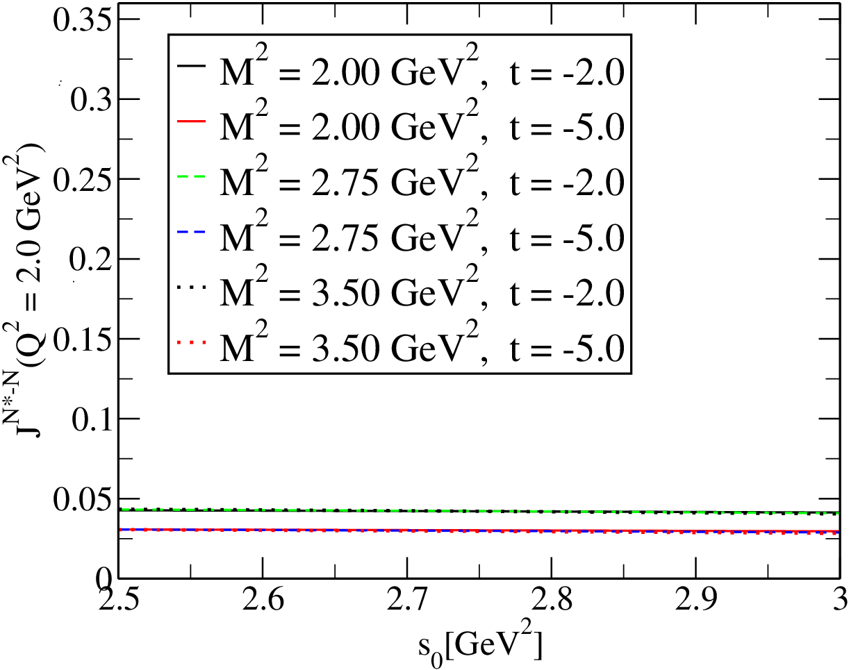
In Figs. (1)-(3), we plot the dependence of the GFFs $A^{N^{*}-N}$ ( $Q^{2}$ ), $J^{N^{*}-N}$ ( $Q^{2}$ ), $D^{N^{*}-N}$ ( $Q^{2}$ ) and $\bar{c}^{N^{*}-N}$ ( $Q^{2}$ ) on different parameters for the various values of the arbitrary mixing parameter $t$ and other parameters in their working regions for two sets of the distribution amplitudes for the $N^{*}$ baryon. As it can be seen from Figs. (1) and (2), the obtained values of the GFFs are approximately independent of the continuum threshold $s_{0}$ and Borel mass parameter $M^{2}$ on their working regions. Therefore, for numerical calculations of the central values of GFFs we will use the central values of the $M^{2}$ and $s_{0}$ . The LCSR method is reliable only $Q^{2}>1.0$ GeV². However, the mass corrections of the distribution amplitudes $\sim m^{2}_{N^{*}}/Q^{2}$ become quite large for $Q^{2}<2.0$ GeV² namely the LCSR turn out to be unreliable. Therefore, for GFFs, we expect the LCSR to operate efficiently and effectively in the $2.0$ GeV ${}^{2}\leq Q^{2}\leq 6.0$ GeV² region. In Fig. 3, we present the $Q^{2}$ dependency of the GFFs on the fixed Borel mass parameter and continuum threshold and various values of the arbitrary mixing parameter $t$ . We see that GFFs smoothly vary in terms of $Q^{2}$ as expected. We also observe that the GFFs $A^{N^{*}-N}$ ( $Q^{2}$ ), $J^{N^{*}-N}$ ( $Q^{2}$ ) and $D^{N^{*}-N}$ ( $Q^{2}$ ) are sensitive to the variations of the mixing parameter $t$ for both sets. The $\bar{c}^{N^{*}-N}$ ( $Q^{2}$ ) form factor is obtained using only the first set of the distribution amplitudes. The second set of the distribution amplitudes gives unphysical results for this form factor (the form factor changes its sign in the region under consideration), therefore it is not presented.

To extend the behavior of GFFs to the region $0\leq Q^{2}<2$ we need to use some fit parametrizations. Our numerical calculations show that the GFFs of the $N^{*}\rightarrow N$ transition can be properly characterized using the p-pole fit function

\displaystyle{\cal F}(Q^{2})=\frac{{\cal F}(0)}{\Big(1+Q^{2}/(p\,m^{2}_{p})\Big)^{p}}.

(20)

Our results for the fit parameters of the $N^{*}\rightarrow N$ transition GFFs are presented in Table 2. The results, obtained by using two sets, are found to be quite different from each other. As it can be see from the Table 1, the main difference between two sets of the distribution amplitudes is the numerical values for the shape parameters $\eta_{10}$ and $\eta_{11}$ , which are connected to the three quark wave functions of the p-wave $N^{*}$ baryon. As a result we find that the $N^{*}\rightarrow N$ transition GFFs depend strongly to the input parameters of the distribution amplitudes of the $N^{*}$ baryon that parametrize the relative orbital angular momentum of the quarks. There are no theoretical predictions for the transition GFFs under study in the literature to be compared with our results. The $D(Q^{2})$ GFF of the $N^{*}$ has recently been obtained by means of the Bag model, $D(Q^{2}=0)=-12.97$ Neubelt:2019sou. Any future experimental data will help us gain useful knowledge on the DAs of the $N^{*}$ state and its nature and internal structure.

Table 2: The obtained numerical results for the parameters of the GFFs by using the p-pole fit functions.

LCSR-1

LCSR-2

Form Factors

{\cal F}(0)

m_{p}

(GeV)

{\cal F}(0)

m_{p}

(GeV)

A^{N^{*}-N}

(

Q^{2}

)

~~1.33\pm 0.13

1.30\pm 0.10

3.0-3.4

~~0.63\pm 0.10

1.32\pm 0.10

3.0-3.4

J^{N^{*}-N}

(

Q^{2}

)

~~0.27\pm 0.07

1.13\pm 0.10

3.0-3.4

~~0.13\pm 0.05

1.17\pm 0.11

2.9-3.3

D^{N^{*}-N}

(

Q^{2}

)

-8.20\pm 2.02

1.14\pm 0.10

3.6-4.0

-6.91\pm 1.80

1.02\pm 0.09

3.2-3.6

\bar{c}^{N^{*}-N}

(

Q^{2}

)

-0.40\pm 0.06

1.18\pm 0.10

3.0-3.5

-

-

-

IV Summary and Concluding Remarks

We applied the quark part of the symmetric energy-momentum tensor current to compute, for the first time, the GFFs of the $N(1535)\rightarrow N$ transition with the help of the LCSR approach. Studying the GFFs of the particles give valuable knowledge about the total angular momentum, spatial distribution of energy, pressure and shear forces inside the particles, etc. In numerical analysis, we used two different sets of shape parameters in the distribution amplitudes of the $N(1535)$ state and took into account the most general form of the nucleon’s interpolating current. It is seen that the momentum squared dependence of the gravitational form factors can be well described by a p-pole fit function. The results obtained by using two sets have been found to be quite different from each other. We found that the values of the $N(1535)\rightarrow N$ transition GFFs highly depend on the input parameters of the distribution amplitudes of the $N(1535)$ state that parameterize relative orbital angular momentum of the quarks. As previously mentioned, we calculated the $N(1535)\rightarrow N$ transition GFFs for the first time in the literature. Therefore, there are no experimental data or theoretical predictions to be compared with the results obtained in this study. Calculations of the GFFs from different methods and approaches are of great importance. Such calculations and comparison of the obtained results with each other will not only help us get useful information on the DAs of the $N^{*}$ state, but also experimental groups for measuring the values of the related GFFs.

V Acknowledgments

U. Ö. acknowledges the support of the Scientific and Technological Research Council of Turkey (TUBITAK) provided through the 2218-National Postdoctoral Research Scholarship Program.

Appendix A: Distribution amplitudes of $N^{\ast}$ state

In this appendix, we present the explicit forms of $N^{*}$ DAs maxiphd:

			$\displaystyle 4\langle 0\left\|\epsilon^{abc}u_{\alpha}^{a}(a_{1}x)d_{\beta}^{b}(a_{2}x)d_{\gamma}^{c}(a_{3}x)\right\|N^{\ast}(p)\rangle$
		$\displaystyle=$	$\displaystyle\!\!\!\mathcal{S}_{1}m_{N^{\ast}}C_{\alpha\beta}N_{\gamma}^{\ast}-\mathcal{S}_{2}m_{N^{\ast}}^{2}C_{\alpha\beta}(\hbox to0.0pt{/\hss}xN^{\ast})_{\gamma}$
		$\displaystyle+$	$\displaystyle\!\!\!\mathcal{P}_{1}m_{N^{\ast}}(\gamma_{5}C)_{\alpha\beta}(\gamma_{5}N^{\ast})_{\gamma}+\mathcal{P}_{2}m_{N^{\ast}}^{2}(\gamma_{5}C)_{\alpha\beta}(\gamma_{5}\hbox to0.0pt{/\hss}xN^{\ast})_{\gamma}-\left(\mathcal{V}_{1}+\frac{x^{2}m_{N^{\ast}}^{2}}{4}\mathcal{V}_{1}^{M}\right)(\hbox to0.0pt{/\hss}pC)_{\alpha\beta}N_{\gamma}^{\ast}$
		$\displaystyle+$	$\displaystyle\!\!\!\mathcal{V}_{2}m_{N^{\ast}}(\hbox to0.0pt{/\hss}pC)_{\alpha\beta}(\hbox to0.0pt{/\hss}xN^{\ast})_{\gamma}+\mathcal{V}_{3}m_{N^{\ast}}(\gamma_{\mu}C)_{\alpha\beta}(\gamma^{\mu}N^{\ast})_{\gamma}-\mathcal{V}_{4}m_{N^{\ast}}^{2}(\hbox to0.0pt{/\hss}xC)_{\alpha\beta}N_{\gamma}^{\ast}$
		$\displaystyle-$	$\displaystyle\!\!\!\mathcal{V}_{5}m_{N^{\ast}}^{2}(\gamma_{\mu}C)_{\alpha\beta}(i\sigma^{\mu\nu}x_{\nu}N^{\ast})_{\gamma}+\mathcal{V}_{6}m_{N^{\ast}}^{3}(\hbox to0.0pt{/\hss}xC)_{\alpha\beta}(\hbox to0.0pt{/\hss}xN^{\ast})_{\gamma}$
		$\displaystyle-$	$\displaystyle\!\!\!\left(\mathcal{A}_{1}+\frac{x^{2}m_{N^{\ast}}^{2}}{4}\mathcal{A}_{1}^{M}\right)(\hbox to0.0pt{/\hss}p\gamma_{5}C)_{\alpha\beta}(\gamma N^{\ast})_{\gamma}+\mathcal{A}_{2}m_{N^{\ast}}(\hbox to0.0pt{/\hss}p\gamma_{5}C)_{\alpha\beta}(\hbox to0.0pt{/\hss}x\gamma_{5}N^{\ast})_{\gamma}+\mathcal{A}_{3}m_{N^{\ast}}(\gamma_{\mu}\gamma_{5}C)_{\alpha\beta}(\gamma^{\mu}\gamma_{5}N^{\ast})_{\gamma}$
		$\displaystyle-$	$\displaystyle\!\!\!\mathcal{A}_{4}m_{N^{\ast}}^{2}(\hbox to0.0pt{/\hss}x\gamma_{5}C)_{\alpha\beta}(\gamma_{5}N^{\ast})_{\gamma}-\mathcal{A}_{5}m_{N^{\ast}}^{2}(\gamma_{\mu}\gamma_{5}C)_{\alpha\beta}(i\sigma^{\mu\nu}x_{\nu}\gamma_{5}N^{\ast})_{\gamma}+\mathcal{A}_{6}m_{N^{\ast}}^{3}(\hbox to0.0pt{/\hss}x\gamma_{5}C)_{\alpha\beta}(\hbox to0.0pt{/\hss}x\gamma_{5}N^{\ast})_{\gamma}$
		$\displaystyle-$	$\displaystyle\!\!\!\left(\mathcal{T}_{1}+\frac{x^{2}m_{N^{\ast}}^{2}}{4}\mathcal{T}_{1}^{M}\right)(i\sigma_{\mu\nu}p_{\nu}C)_{\alpha\beta}(\gamma^{\mu}N^{\ast})_{\gamma}+\mathcal{T}_{2}m_{N^{\ast}}(i\sigma_{\mu\nu}x^{\mu}p^{\nu}C)_{\alpha\beta}N_{\gamma}^{\ast}$
		$\displaystyle+$	$\displaystyle\!\!\!\mathcal{T}_{3}m_{N^{\ast}}(\sigma_{\mu\nu}C)_{\alpha\beta}(\sigma^{\mu\nu}N^{\ast})_{\gamma}+\mathcal{T}_{4}m_{N^{\ast}}(\sigma_{\mu\nu}p^{\nu}C)_{\alpha\beta}(\sigma^{\mu\rho}x_{\rho}N^{\ast})_{\gamma}$
		$\displaystyle-$	$\displaystyle\!\!\!\mathcal{T}_{5}m_{N^{\ast}}^{2}(i\sigma_{\mu\nu}x^{\nu}C)_{\alpha\beta}(\gamma^{\mu}N^{\ast})_{\gamma}-\mathcal{T}_{6}m_{N^{\ast}}^{2}(i\sigma_{\mu\nu}x^{\mu}p^{\nu}C)_{\alpha\beta}(\hbox to0.0pt{/\hss}xN^{\ast})_{\gamma}$
		$\displaystyle-$	$\displaystyle\!\!\!\mathcal{T}_{7}m_{N^{\ast}}^{2}(\sigma_{\mu\nu}C)_{\alpha\beta}(\sigma^{\mu\nu}\hbox to0.0pt{/\hss}xN^{\ast})_{\gamma}+\mathcal{T}_{8}m_{N^{\ast}}^{3}(\sigma_{\mu\nu}x^{\nu}C)_{\alpha\beta}(\sigma^{\mu\rho}x_{\rho}N^{\ast})_{\gamma}~.$

The “calligraphic” functions can be represented with respect to the functions of the specific twists as:

	$\displaystyle\mathcal{S}_{1}=$	$\displaystyle S_{1},\hskip 99.58464pt2p.x\mathcal{S}_{2}=S_{1}-S_{2},$
	$\displaystyle\mathcal{P}_{1}=$	$\displaystyle P_{1},\hskip 99.58464pt2p.x\mathcal{P}_{2}=P_{1}-P_{2},$
	$\displaystyle\mathcal{V}_{1}=$	$\displaystyle V_{1},\hskip 99.58464pt2p.x\mathcal{V}_{2}=V_{1}-V_{2}-V_{3},$
	$\displaystyle 2\mathcal{V}_{3}=$	$\displaystyle V_{3},\hskip 99.58464pt4p.x\mathcal{V}_{4}=-2V_{1}+V_{3}+V_{4}+2V_{5},$
	$\displaystyle 4p.x\mathcal{V}_{5}=$	$\displaystyle V_{4}-V_{3},\hskip 71.13188pt4(p.x)^{2}\mathcal{V}_{6}=-V_{1}+V_{2}+V_{3}+V_{4}+V_{5}-V_{6}$
	$\displaystyle\mathcal{A}_{1}=$	$\displaystyle A_{1},\hskip 99.58464pt2p.x\mathcal{A}_{2}=-A_{1}+A_{2}-A_{3},$
	$\displaystyle 2\mathcal{A}_{3}=$	$\displaystyle A_{3},\hskip 99.58464pt4p.x\mathcal{A}_{4}=-2A_{1}-A_{3}-A_{4}+2A_{5},$
	$\displaystyle 4p.x\mathcal{A}_{5}=$	$\displaystyle A_{3}-A_{4},\hskip 71.13188pt4(p.x)^{2}\mathcal{A}_{6}=A_{1}-A_{2}+A_{3}+A_{4}-A_{5}+A_{6}$
	$\displaystyle\mathcal{T}_{1}=$	$\displaystyle T_{1},\hskip 99.58464pt2p.x\mathcal{T}_{2}=T_{1}+T_{2}-2T_{3},$
	$\displaystyle 2\mathcal{T}_{3}=$	$\displaystyle T_{7},\hskip 99.58464pt2p.x\mathcal{T}_{4}=T_{1}-T_{2}-2T_{7},$
	$\displaystyle 2p.x\mathcal{T}_{5}=$	$\displaystyle-T_{1}+T_{5}+2T_{8},\hskip 28.45274pt4(p.x)^{2}\mathcal{T}_{6}=2T_{2}-2T_{3}-2T_{4}+2T_{5}+2T_{7}+2T_{8},$
	$\displaystyle 4p.x\mathcal{T}_{7}=$	$\displaystyle T_{7}-T_{8},\hskip 71.13188pt4(p.x)^{2}\mathcal{T}_{8}=-T_{1}+T_{2}+T_{5}-T_{6}+2T_{7}+2T_{8},$

where $V_{i},A_{i},T_{i},S_{i}$ and $P_{i}$ are vector, axialvector, tensor, scalar and pesudoscalar distribution amplitudes, respectively. The explicit expressions of these functions are given as follows

$\displaystyle V_{1}(x_{i},\mu)$	$\displaystyle=$	$\displaystyle 120x_{1}x_{2}x_{3}[\phi_{3}^{0}(\mu)+\phi_{3}^{+}(\mu)(1-3x_{3})],$
$\displaystyle V_{2}(x_{i},\mu)$	$\displaystyle=$	$\displaystyle 24x_{1}x_{2}[\phi_{4}^{0}(\mu)+\phi_{4}^{+}(\mu)(1-5x_{3})],$
$\displaystyle V_{3}(x_{i},\mu)$	$\displaystyle=$	$\displaystyle 12x_{3}\{\psi_{4}^{0}(\mu)(1-x_{3})+\psi_{4}^{-}(\mu)[x_{1}^{2}+x_{2}^{2}-x_{3}(1-x_{3})]$
		$\displaystyle+\psi_{4}^{+}(\mu)(1-x_{3}-10x_{1}x_{2})\},$
$\displaystyle V_{4}(x_{i},\mu)$	$\displaystyle=$	$\displaystyle 3\{\psi_{5}^{0}(\mu)(1-x_{3})+\psi_{5}^{-}(\mu)[2x_{1}x_{2}-x_{3}(1-x_{3})]$
		$\displaystyle+\psi_{5}^{+}(\mu)[1-x_{3}-2(x_{1}^{2}+x_{2}^{2})]\},$
$\displaystyle V_{5}(x_{i},\mu)$	$\displaystyle=$	$\displaystyle 6x_{3}[\phi_{5}^{0}(\mu)+\phi_{5}^{+}(\mu)(1-2x_{3})],$
$\displaystyle V_{6}(x_{i},\mu)$	$\displaystyle=$	$\displaystyle 2[\phi_{6}^{0}(\mu)+\phi_{6}^{+}(\mu)(1-3x_{3})],$
$\displaystyle A_{1}(x_{i},\mu)$	$\displaystyle=$	$\displaystyle 120x_{1}x_{2}x_{3}\phi_{3}^{-}(\mu)(x_{2}-x_{1}),$
$\displaystyle A_{2}(x_{i},\mu)$	$\displaystyle=$	$\displaystyle 24x_{1}x_{2}\phi_{4}^{-}(\mu)(x_{2}-x_{1}),$
$\displaystyle A_{3}(x_{i},\mu)$	$\displaystyle=$	$\displaystyle 12x_{3}(x_{2}-x_{1})\{(\psi_{4}^{0}(\mu)+\psi_{4}^{+}(\mu))+\psi_{4}^{-}(\mu)(1-2x_{3})\},$
$\displaystyle A_{4}(x_{i},\mu)$	$\displaystyle=$	$\displaystyle 3(x_{2}-x_{1})\{-\psi_{5}^{0}(\mu)+\psi_{5}^{+}(\mu)(1-2x_{3})+\psi_{5}^{-}(\mu)x_{3}\},$
$\displaystyle A_{5}(x_{i},\mu)$	$\displaystyle=$	$\displaystyle 6x_{3}(x_{2}-x_{1})\phi_{5}^{-}(\mu)$
$\displaystyle A_{6}(x_{i},\mu)$	$\displaystyle=$	$\displaystyle 2(x_{2}-x_{1})\phi_{6}^{-}(\mu),$
$\displaystyle T_{1}(x_{i},\mu)$	$\displaystyle=$	$\displaystyle 120x_{1}x_{2}x_{3}[\phi_{3}^{0}(\mu)+\frac{1}{2}(\phi_{3}^{-}-\phi_{3}^{+})(\mu)(1-3x_{3})],$
$\displaystyle T_{2}(x_{i},\mu)$	$\displaystyle=$	$\displaystyle 24x_{1}x_{2}[\xi_{4}^{0}(\mu)+\xi_{4}^{+}(\mu)(1-5x_{3})],$
$\displaystyle T_{3}(x_{i},\mu)$	$\displaystyle=$	$\displaystyle 6x_{3}\{(\xi_{4}^{0}+\phi_{4}^{0}+\psi_{4}^{0})(\mu)(1-x_{3})+(\xi_{4}^{-}+\phi_{4}^{-}-\psi_{4}^{-})(\mu)[x_{1}^{2}+x_{2}^{2}-x_{3}$
		$\displaystyle(1-x_{3})]+(\xi_{4}^{+}+\phi_{4}^{+}+\psi_{4}^{+})(\mu)(1-x_{3}-10x_{1}x_{2})\},$
$\displaystyle T_{4}(x_{i},\mu)$	$\displaystyle=$	$\displaystyle\frac{3}{2}\{(\xi_{5}^{0}+\phi_{5}^{0}+\psi_{5}^{0})(\mu)(1-x_{3})+(\xi_{5}^{-}+\phi_{5}^{-}-\psi_{5}^{-})(\mu)[2x_{1}x_{2}-x_{3}(1-x_{3})]$
		$\displaystyle+(\xi_{5}^{+}+\phi_{5}^{+}+\psi_{5}^{+})(\mu)(1-x_{3}-2(x_{1}^{2}+x_{2}^{2}))\},$
$\displaystyle T_{5}(x_{i},\mu)$	$\displaystyle=$	$\displaystyle 6x_{3}[\xi_{5}^{0}(\mu)+\xi_{5}^{+}(\mu)(1-2x_{3})],$
$\displaystyle T_{6}(x_{i},\mu)$	$\displaystyle=$	$\displaystyle 2[\phi_{6}^{0}(\mu)+\frac{1}{2}(\phi_{6}^{-}-\phi_{6}^{+})(\mu)(1-3x_{3})],$
$\displaystyle T_{7}(x_{i},\mu)$	$\displaystyle=$	$\displaystyle 6x_{3}\{(-\xi_{4}^{0}+\phi_{4}^{0}+\psi_{4}^{0})(\mu)(1-x_{3})+(-\xi_{4}^{-}+\phi_{4}^{-}-\psi_{4}^{-})(\mu)[x_{1}^{2}+x_{2}^{2}$
		$\displaystyle-x_{3}(1-x_{3})](1-x_{3})]+(-\xi_{4}^{+}+\phi_{4}^{+}+\psi_{4}^{+})(\mu)(1-x_{3}-10x_{1}x_{2})\},$
$\displaystyle T_{8}(x_{i},\mu)$	$\displaystyle=$	$\displaystyle\frac{3}{2}\{(-\xi_{5}^{0}+\phi_{5}^{0}+\psi_{5}^{0})(\mu)(1-x_{3})+(-\xi_{5}^{-}+\phi_{5}^{-}-\psi_{5}^{-})(\mu)[2x_{1}x_{2}-$
		$\displaystyle+x_{3}(1-x_{3})](1-x_{3})]+(-\xi_{5}^{+}+\phi_{5}^{+}+\psi_{5}^{+})(\mu)(1-x_{3}-2(x_{1}^{2}+x_{2}^{2}))\},$
$\displaystyle S_{1}(x_{i},\mu)$	$\displaystyle=$	$\displaystyle 6x_{3}(x_{2}-x_{1})\left[(\xi_{4}^{0}+\phi_{4}^{0}+\psi_{4}^{0}+\xi_{4}^{+}+\phi_{4}^{+}+\psi_{4}^{+})(\mu)\right.$
		$\displaystyle\left.+(\xi_{4}^{-}+\phi_{4}^{-}-\psi_{4}^{-})(\mu)(1-2x_{3})\right]$
$\displaystyle S_{2}(x_{i},\mu)$	$\displaystyle=$	$\displaystyle\frac{3}{2}(x_{2}-x_{1})\left[-\left(\psi_{5}^{0}+\phi_{5}^{0}+\xi_{5}^{0}\right)(\mu)+\left(\xi_{5}^{-}+\phi_{5}^{-}-\psi_{5}^{-}\right)(\mu)x_{3}\right.$
		$\displaystyle\left.+\left(\xi_{5}^{+}+\phi_{5}^{+}+\psi_{5}^{0}\right)(\mu)(1-2x_{3})\right]$
$\displaystyle P_{1}(x_{i},\mu)$	$\displaystyle=$	$\displaystyle 6x_{3}(x_{2}-x_{1})\left[(\xi_{4}^{0}-\phi_{4}^{0}-\psi_{4}^{0}+\xi_{4}^{+}-\phi_{4}^{+}-\psi_{4}^{+})(\mu)\right.$
		$\displaystyle\left.+(\xi_{4}^{-}-\phi_{4}^{-}+\psi_{4}^{-})(\mu)(1-2x_{3})\right]$
$\displaystyle P_{2}(x_{i},\mu)$	$\displaystyle=$	$\displaystyle\frac{3}{2}(x_{2}-x_{1})\left[\left(\psi_{5}^{0}+\psi_{5}^{0}-\xi_{5}^{0}\right)(\mu)+\left(\xi_{5}^{-}-\phi_{5}^{-}+\psi_{5}^{-}\right)(\mu)x_{3}\right.$
		$\displaystyle\left.+\left(\xi_{5}^{+}-\phi_{5}^{+}-\psi_{5}^{+}\right)(\mu)(1-2x_{3})\right]\,.$
$\displaystyle{\cal V}_{1}^{M}(x_{2})$	$\displaystyle=$	$\displaystyle\int\limits_{0}^{1-x_{2}}dx_{1}V_{1}^{M}(x_{1},x_{2},1-x_{1}-x_{2})=\frac{x_{2}^{2}}{24}\left[f_{N^{\ast}}C_{f}^{u}(x_{2})+\lambda_{1}^{N^{\ast}}C_{\lambda}^{u}(x_{2})\right],$
$\displaystyle{\cal A}_{1}^{M}(x_{2})$	$\displaystyle=$	$\displaystyle\int_{0}^{1-x_{2}}dx_{1}A_{1}^{M}(x_{1},x_{2},1-x_{1}-x_{2})=\frac{x_{2}^{2}}{24}(1-x_{2})^{3}\left[f_{N^{\ast}}D_{f}^{u}(x_{2})+\lambda_{1}^{N^{\ast}}D_{\lambda}^{u}(x_{2})\right],$
$\displaystyle{\cal T}_{1}^{M}(x_{2})$	$\displaystyle=$	$\displaystyle\int_{0}^{1-x_{2}}dx_{1}T_{1}^{M}(x_{1},x_{2},1-x_{1}-x_{2})=\frac{x^{2}}{48}\left[f_{N^{\ast}}E_{f}^{u}(x_{2})+\lambda_{1}^{N^{\ast}}E_{\lambda}^{u}(x_{2})\right].$

The subsequent functions come across to the above DAs and they can be parametrized with respect to the independent parameters, such as $f_{N^{\ast}}$ , $\lambda_{1}$ , $\lambda_{2}$ , $f_{1}^{u}$ , $f_{1}^{d}$ , $f_{2}^{d}$ , $A_{1}^{u}$ and $V_{1}^{d}$ :

		$\displaystyle\phi_{3}^{0}=\phi_{6}^{0}=f_{N^{\ast}}$
		$\displaystyle\phi_{4}^{0}=\phi_{5}^{0}={1\over 2}(f_{N^{\ast}}+\lambda_{1}^{N^{\ast}})$
		$\displaystyle\xi_{4}^{0}=\xi_{5}^{0}={1\over 6}\lambda_{2}^{N^{\ast}}$
		$\displaystyle\psi_{4}^{0}=\psi_{5}^{0}={1\over 2}(f_{N^{\ast}}-\lambda_{1}^{N^{\ast}}),$
		$\displaystyle\phi_{3}^{-}={21\over 2}f_{N^{\ast}}A_{1}^{u},~~\phi_{3}^{+}={7\over 2}f_{N^{\ast}}(1-V_{1}^{d}),$
		$\displaystyle\phi_{4}^{+}={1\over 4}\left[f_{N^{\ast}}(3-10V_{1}^{d})+\lambda_{1}^{N^{\ast}}(3-10f_{1}^{d})\right],$
		$\displaystyle\phi_{4}^{-}=-{5\over 4}\left[f_{N^{\ast}}(1-2A_{1}^{u})-\lambda_{1}^{N^{\ast}}(1-2f_{1}^{d}-4f_{1}^{u})\right],$
		$\displaystyle\psi_{4}^{+}=-{1\over 4}\left[f_{N^{\ast}}(2+5A_{1}^{u}-5V_{1}^{d})-\lambda_{1}^{N^{\ast}}(2-5f_{1}^{d}-5f_{1}^{u})\right],$
		$\displaystyle\psi_{4}^{-}={5\over 4}\left[f_{N^{\ast}}(2-A_{1}^{u}-3V_{1}^{d})-\lambda_{1}^{N^{\ast}}(2-7f_{1}^{d}+f_{1}^{u})\right],$
		$\displaystyle\xi_{4}^{+}={1\over 16}\lambda_{2}^{N^{\ast}}(4-15f_{2}^{d}),$
		$\displaystyle\xi_{4}^{-}={5\over 16}\lambda_{2}^{N^{\ast}}(4-15f_{2}^{d}),$
		$\displaystyle\phi_{5}^{+}=-{5\over 6}\left[f_{N^{\ast}}(3+4V_{1}^{d})-\lambda_{1}^{N^{\ast}}(1-4f_{1}^{d})\right],$
		$\displaystyle\phi_{5}^{-}=-{5\over 3}\left[f_{N^{\ast}}(1-2A_{1}^{u})-\lambda_{1}^{N^{\ast}}(f_{1}^{d}-f_{1}^{u})\right],$
		$\displaystyle\psi_{5}^{+}=-{5\over 6}\left[f_{N^{\ast}}(5+2A_{1}^{u}-2V_{1}^{d})-\lambda_{1}^{N^{\ast}}(1-2f_{1}^{d}-2f_{1}^{u})\right],$
		$\displaystyle\psi_{5}^{-}={5\over 3}\left[f_{N^{\ast}}(2-A_{1}^{u}-3V_{1}^{d})+\lambda_{1}^{N^{\ast}}(f_{1}^{d}-f_{1}^{u})\right],$
		$\displaystyle\xi_{5}^{+}={5\over 36}\lambda_{2}^{N^{\ast}}(2-9f_{2}^{d})~,$
		$\displaystyle\xi_{5}^{-}=-{5\over 4}\lambda_{2}^{N^{\ast}}f_{2}^{d},$
		$\displaystyle\phi_{6}^{+}={1\over 2}\left[f_{N^{\ast}}(1-4V_{1}^{d})-\lambda_{1}^{N^{\ast}}(1-2f_{1}^{d})\right],$
		$\displaystyle\phi_{6}^{-}={1\over 2}\left[f_{N^{\ast}}(1+4A_{1}^{d})+\lambda_{1}^{N^{\ast}}(1-4f_{1}^{d}-2f_{1}^{u})\right],$
		$\displaystyle C_{f}^{u}(x_{2})=(1-x_{2})^{3}\Big[113+495x_{2}-552x_{2}^{2}-10A_{1}^{u}(1-3x_{2})+2V_{1}^{d}(113-951x_{2}+828x_{2}^{2})\Big]~,$
		$\displaystyle C_{\lambda}^{u}(x_{2})=-(1-x_{2})^{3}\Big[13-20f_{1}^{d}+3x_{2}+10f_{1}^{u}(1\!-\!3x_{2})\Big]~.$
		$\displaystyle D_{f}^{u}(x_{2})=11+45x_{2}-2A_{1}^{u}(113-951x_{2}+828x_{2}^{2})+10V_{1}^{d}(1-30x_{2})~,$
		$\displaystyle D_{\lambda}^{u}(x_{2})=29-45x_{2}-10f_{1}^{u}(7-9x_{2})-20f_{1}^{d}(5-6x_{2})~.$
		$\displaystyle E_{f}^{u}(x_{2})=-\Big\{(1-x_{2})\Big[3(439+71x_{2}-621x_{2}^{2}+587x_{2}^{3}-184x_{2}^{4})+4A_{1}^{u}(1-x_{2})^{2}(59-483x_{2}+414x_{2}^{2})$
		$\displaystyle-4V_{1}^{d}(1301-619x_{2}-769x_{2}^{2}+1161x_{2}^{3}-414x_{2}^{4})\Big]\Big\}-12(73-220V_{1}^{d})\ln[x_{2}]~,$
		$\displaystyle E_{\lambda}^{u}(x_{2})=-\Big\{(1-x_{2})\Big[5-211x_{2}+281x_{2}^{2}-111x_{2}^{3}+10(1+61x_{2}-83x_{2}^{2}+33x_{2}^{3})f_{1}^{d}$
		$\displaystyle-40(1-x_{2})^{2}(2-3x_{2})f_{1}^{u}\Big]\Big\}-12(3-10f_{1}^{d})\ln[x_{2}],$

where the parameters $A_{1}^{u},~V_{1}^{d},~f_{1}^{d},~f_{1}^{u}$ , and $f_{2}^{d}$ are defined as maxiphd

		$\displaystyle A_{1}^{u}=\varphi_{10}+\varphi_{11}~,$
		$\displaystyle V_{1}^{d}={1\over 3}-\varphi_{10}+{1\over 3}\varphi_{11}~,$
		$\displaystyle f_{1}^{u}={1\over 10}-{1\over 6}{f_{N^{\ast}}\over\lambda_{1}^{N^{\ast}}}-{3\over 5}\eta_{10}-{1\over 3}\eta_{11}~,$
		$\displaystyle f_{1}^{d}={3\over 10}-{1\over 6}{f_{N^{\ast}}\over\lambda_{1}^{N^{\ast}}}+{1\over 5}\eta_{10}-{1\over 3}\eta_{11}~,$
		$\displaystyle f_{2}^{d}={4\over 15}+{2\over 5}\xi_{10}~.$

Appendix B: Explicit forms of the functions $\varPi_{i}$ for the $N^{*}\rightarrow N$ transition

$\displaystyle\varPi_{1}^{QCD}(Q^{2})$	$\displaystyle=\frac{m_{N^{*}}}{2}\int_{0}^{1}\frac{x_{2}^{2}\,dx_{2}}{(q-px_{2})^{2}}\int_{0}^{1-x_{2}}dx_{1}\Big[3(1-t)[-A_{3}-V_{3}]\,+\,(1+t)[P_{1}+S_{1}+T_{1}-T_{7}]\Big](x_{1},x_{2},1-x_{1}-x_{2})$
	$\displaystyle+\frac{m_{N^{*}}}{2}\int_{0}^{1}\frac{x_{3}^{2}\,dx_{3}}{(q-px_{3})^{2}}\int_{0}^{1-x_{3}}dx_{3}\Big[(1-t)[-A_{3}-V_{3}]\,+\,(1+t)[P_{1}+S_{1}+T_{1}-T_{7}]\Big](x_{1},1-x_{1}-x_{3},x_{3})$
	$\displaystyle+\frac{m^{3}_{N^{*}}}{2}\int_{0}^{1}\frac{x_{2}^{2}\,dx_{2}}{(q-px_{2})^{4}}\int_{0}^{1-x_{2}}dx_{1}\Big[2(1-t)[2A_{1}^{M}+V_{1}^{M}]\,+\,3\,(1+t)T_{1}^{M}\Big](x_{1},x_{2},1-x_{1}-x_{2})$
	$\displaystyle+\frac{m_{N^{*}}}{2}\int_{0}^{1}\frac{\alpha\,d\alpha}{(q-p\alpha)^{2}}\int_{\alpha}^{1}dx_{2}\int_{0}^{1-x_{2}}dx_{1}\Big[(1-t)[-3A_{1}+3A_{2}-3A_{3}+V_{1}-V_{2}-V_{3}]$
	$\displaystyle+\,(1+t)[5T_{1}-T_{2}-3T_{3}-7T_{7}]\Big](x_{1},x_{2},1-x_{1}-x_{2})$
	$\displaystyle+\frac{m_{N^{*}}}{2}\int_{0}^{1}\frac{\alpha\,d\alpha}{(q-p\alpha)^{2}}\int_{\alpha}^{1}dx_{3}\int_{0}^{1-x_{3}}dx_{1}\Big[(1+t)[3T_{1}+T_{2}-2T_{3}-T_{7}]\Big](x_{1},1-x_{1}-x_{3},x_{3})$
	$\displaystyle+\frac{m^{3}_{N^{*}}}{2}\int_{0}^{1}\frac{\alpha^{3}\,d\alpha}{(q-p\alpha)^{4}}\int_{\alpha}^{1}dx_{2}\int_{0}^{1-x_{2}}dx_{1}\Big[(1-t)[-3A_{1}+A_{2}-2A_{3}+A_{4}+2A_{5}+V_{1}-V_{2}-2V_{3}+V_{4}]$
	$\displaystyle+\,(1+t)[P_{1}-P_{2}+S_{1}-S_{2}+2T_{1}-3T_{2}+2T_{3}-T_{5}-6T_{7}]\Big](x_{1},x_{2},1-x_{1}-x_{2})$
	$\displaystyle+\frac{m^{3}_{N^{*}}}{2}\int_{0}^{1}\frac{\alpha^{3}\,d\alpha}{(q-p\alpha)^{4}}\int_{\alpha}^{1}dx_{3}\int_{0}^{1-x_{3}}dx_{1}\Big[(1-t)[-A_{1}+A_{2}-2A_{3}+A_{4}+V_{1}-V_{2}-V_{3}+V_{4}]$
	$\displaystyle\,+\,(1+t)[P_{1}-P_{2}+S_{1}-S_{2}+2T_{1}-3T_{2}+2T_{3}-T_{5}-6T_{7}]\Big](x_{1},1-x_{1}-x_{3},x_{3})$
	$\displaystyle+\frac{m^{3}_{N^{*}}}{2}\int_{0}^{1}\frac{\beta^{2}\,d\beta}{(q-p\beta)^{4}}\int_{0}^{\beta}d\alpha\int_{\alpha}^{1}dx_{2}\int_{0}^{1-x_{2}}dx_{1}\Big[2(1-t)[-2A_{1}+2A_{2}-2A_{3}-2A_{4}+2A_{5}-2A_{6}$
	$\displaystyle+V_{1}-V_{2}-V_{3}-V_{4}-V_{5}+V_{6}]\,+\,(1+t)[7T_{1}-2T_{2}-5T_{3}-5T_{4}-2T_{5}+7T_{6}-9T_{7}$
	$\displaystyle-9T_{8}]\Big](x_{1},x_{2},1-x_{1}-x_{2})$
	$\displaystyle+\frac{m^{3}_{N^{*}}}{2}\int_{0}^{1}\frac{\beta^{2}\,d\beta}{(q-p\beta)^{4}}\int_{0}^{\beta}d\alpha\int_{\alpha}^{1}dx_{3}\int_{0}^{1-x_{3}}dx_{1}\Big[(1+t)[2T_{1}+T_{2}-3T_{3}-3T_{4}+T_{5}+T_{6}-T_{7}$
	$\displaystyle-T_{8}]\Big](x_{1},1-x_{1}-x_{3},x_{3}),$	(21)
$\displaystyle\varPi_{2}^{QCD}(Q^{2})$	$\displaystyle=-\frac{1}{2}\int_{0}^{1}\frac{1}{(q-px_{2})^{2}}dx_{2}\int_{0}^{1-x_{2}}dx_{1}\Big[(1-t)[A_{1}+V_{1}]\Big](x_{1},x_{2},1-x_{1}-x_{2})$
	$\displaystyle+\frac{m^{2}_{N^{*}}}{2}\int_{0}^{1}\frac{1}{(q-px_{2})^{4}}dx_{2}\int_{0}^{1-x_{2}}dx_{1}\Big[3(1-t)[A_{1}^{M}+V_{1}^{M}]\Big](x_{1},x_{2},1-x_{1}-x_{2})$

	$\displaystyle+\frac{m^{2}_{N^{*}}}{2}\int_{0}^{1}\frac{\alpha^{2}\,d\alpha}{(q-p\alpha)^{4}}\int_{\alpha}^{1}dx_{2}\int_{0}^{1-x_{2}}dx_{1}\Big[(1-t)[-A_{1}-A_{2}-A_{3}+A_{4}+A_{5}-V_{1}+V_{2}+V_{4}]$
	$\displaystyle+\,(1+t)[P_{1}-P_{2}+S_{1}-S_{2}+T_{2}-T_{5}]\Big](x_{1},x_{2},1-x_{1}-x_{2})$
	$\displaystyle+\frac{m^{2}_{N^{*}}}{2}\int_{0}^{1}\frac{\alpha^{2}\,d\alpha}{(q-p\alpha)^{4}}\int_{\alpha}^{1}dx_{3}\int_{0}^{1-x_{3}}dx_{1}\Big[(1-t)[A_{1}-A_{2}+A_{4}-V_{1}+V_{2}+V_{4}]\,+\,(1+t)[P_{1}-P_{2}+S_{1}$
	$\displaystyle-S_{2}+T_{2}-T_{5}]\Big](x_{1},1-x_{1}-x_{3},x_{3})$
	$\displaystyle+\frac{m^{2}_{N^{*}}}{2}\int_{0}^{1}\frac{\beta\,d\beta}{(q-p\beta)^{4}}\int_{0}^{\beta}d\alpha\int_{\alpha}^{1}dx_{2}\int_{0}^{1-x_{2}}dx_{1}\Big[(1+t)[T_{2}-T_{3}-T_{4}+T_{5}+T_{7}+T_{8}]\Big]$
	$\displaystyle\times(x_{1},x_{2},1-x_{1}-x_{2})$
	$\displaystyle+\frac{m^{2}_{N^{*}}}{2}\int_{0}^{1}\frac{\beta\,d\beta}{(q-p\beta)^{4}}\int_{0}^{\beta}d\alpha\int_{\alpha}^{1}dx_{3}\int_{0}^{1-x_{3}}dx_{1}\Big[(1+t)[T_{2}-T_{3}-T_{4}+T_{5}+T_{7}+T_{8}]\Big]$
	$\displaystyle\times(x_{1},1-x_{1}-x_{3},x_{3}),$	(22)
$\displaystyle\varPi_{3}^{QCD}(Q^{2})$	$\displaystyle=\frac{1}{2}\int_{0}^{1}dx_{2}\frac{(1-x_{2})}{(q-px_{2})^{2}}\int_{0}^{1-x_{2}}\Big[(1-t)[A_{1}+V_{1}]\Big](x_{1},x_{2},1-x_{1}-x_{2})$
	$\displaystyle+\frac{1}{2}\int_{0}^{1}dx_{3}\frac{(1-x_{3})}{(q-px_{3})^{2}}\int_{0}^{1-x_{3}}\Big[(1-t)[A_{1}-V_{1}]\Big](x_{1},1-x_{1}-x_{3},x_{3})$
	$\displaystyle+\frac{1}{2}\int_{0}^{1}dx_{2}\frac{(1-x_{2})}{(q-px_{2})^{4}}\int_{0}^{1-x_{2}}\Big[(1-t)[3V_{1}^{M}+3A_{1}^{M}]\Big](x_{1},x_{2},1-x_{1}-x_{2})$
	$\displaystyle+\frac{m^{2}_{N^{*}}}{2}\int_{0}^{1}\frac{d\alpha}{(q-p\alpha)^{4}}\int_{\alpha}^{1}dx_{2}\int_{0}^{1-x_{2}}dx_{1}\Big[(1-t)[-A_{1}-A_{2}-2A_{3}+A_{4}+2A_{5}-V_{1}+V_{2}+V_{4}]$
	$\displaystyle+(1+t)[P_{1}-P_{2}+S_{1}-S_{2}+T_{2}-T_{5}]\Big](x_{1},x_{2},1-x_{1}-x_{2})$
	$\displaystyle+\frac{m^{2}_{N^{*}}}{2}\int_{0}^{1}\frac{d\alpha}{(q-p\alpha)^{4}}\int_{\alpha}^{1}dx_{3}\int_{0}^{1-x_{3}}dx_{1}\Big[(1-t)[-A_{1}-A_{2}+A_{4}-V_{1}+V_{2}+V_{4}]$
	$\displaystyle+(1+t)[P_{1}-P_{2}+S_{1}-S_{2}+T_{2}-T_{5}]\Big](x_{1},1-x_{1}-x_{3},x_{3}))$
	$\displaystyle+\frac{m^{2}_{N^{*}}}{2}\int_{0}^{1}\frac{\alpha(1-\alpha)}{(q-p\alpha)^{4}}d\alpha\int_{\alpha}^{1}dx_{2}\int_{0}^{1-x_{2}}dx_{1}\Big[2(1-t)[-A_{1}-A_{2}-2A_{3}+A_{4}+2A_{5}-V_{1}+V_{2}+V_{4}]$
	$\displaystyle+(1+t)[P_{1}-P_{2}+S_{1}-S_{2}+T_{2}-T_{5}]\Big](x_{1},x_{2},1-x_{1}-x_{2})$
	$\displaystyle+\frac{m^{2}_{N^{*}}}{2}\int_{0}^{1}\frac{\alpha(1-\alpha)}{(q-p\alpha)^{4}}d\alpha\int_{\alpha}^{1}dx_{3}\int_{0}^{1-x_{3}}dx_{1}\Big[(1-t)[A_{1}-A_{2}+A_{4}-V_{1}+V_{2}+V_{4}]$
	$\displaystyle+\,(1+t)[P_{1}-P_{2}+S_{1}-S_{2}-T_{2}-T_{5}]\Big](x_{1},1-x_{1}-x_{3},x_{3}),$
	$\displaystyle+\frac{m^{2}_{N^{*}}}{2}\int_{0}^{1}\frac{(1+\beta)}{(q-p\beta)^{4}}d\beta\int_{0}^{\beta}d\alpha\int_{\alpha}^{1}dx_{2}\int_{0}^{1-x_{2}}dx_{1}(1+t)[T_{2}-T_{3}-T_{4}+T_{5}+T_{7}+T_{8}]$
	$\displaystyle\times(x_{1},x_{2},1-x_{1}-x_{2})$
	$\displaystyle+\frac{m^{2}_{N^{*}}}{2}\int_{0}^{1}\frac{(1+\beta)}{(q-p\beta)^{4}}d\beta\int_{0}^{\beta}d\alpha\int_{\alpha}^{1}dx_{3}\int_{0}^{1-x_{3}}dx_{1}\Big[3(1+t)[T_{2}-T_{3}-T_{4}+T_{5}+T_{7}+T_{8}]\Big]$
	$\displaystyle\times(x_{1},1-x_{1}-x_{3},x_{3}),$	(23)
$\displaystyle\varPi_{4}^{QCD}(Q^{2})$	$\displaystyle=\frac{m^{3}_{N^{*}}}{2}\int_{0}^{1}\frac{dx_{2}}{(p-px_{2})^{2}}\int_{0}^{1-x_{2}}(1+t)T_{1}^{M}(x_{1},x_{2},1-x_{1}-x_{2})$
	$\displaystyle+\frac{m^{3}_{N^{*}}}{8}\int_{0}^{1}\frac{\alpha\,d\alpha}{(q-p\alpha)^{2}}\int_{\alpha}^{1}dx_{2}\int_{0}^{1-x_{2}}dx_{1}\Big[(1-t)[-2A_{1}-2A_{2}-3A_{3}+A_{4}+4A_{5}-2V_{1}+2V_{2}-V_{3}$
	$\displaystyle+3V_{4}]+\,(1+t)[2P_{1}-2P_{2}+2S_{1}-2S_{2}-T_{1}+T_{2}+4T_{3}-4T_{5}-2T_{7}]\Big](x_{1},x_{2},1-x_{1}-x_{2})$

		$\displaystyle+\frac{m^{3}_{N^{*}}}{8}\int_{0}^{1}\frac{\alpha\,d\alpha}{(q-p\alpha)^{2}}\int_{\alpha}^{1}dx_{3}\int_{0}^{1-x_{3}}dx_{1}\Big[-2A_{1}+2A_{2}-3A_{3}+A_{4}+2V_{1}-2V_{2}-3V_{3}+V_{4}]$
		$\displaystyle+\,(1+t)[2P_{1}-2P_{2}+2S_{1}-2S_{2}+T_{1}-T_{2}-3T_{5}-T_{7}]\Big](x_{1},1-x_{1}-x_{3},x_{3})$
		$\displaystyle+\frac{m^{3}_{N^{*}}}{8}\int_{0}^{1}\frac{d\beta}{(q-p\beta)^{2}}\int_{0}^{\beta}d\alpha\int_{\alpha}^{1}dx_{2}\int_{0}^{1-x_{2}}dx_{1}\Big[4\,(1-t)[-A_{1}+A_{2}-A_{3}-A_{4}+A_{5}-A_{6}-V_{1}+V_{2}+V_{3}$
		$\displaystyle+V_{4}+V_{5}-V_{6}]\,+\,(1+t)[T_{1}-T_{2}-T_{5}+T_{6}-2T_{7}-2T_{8}]\Big](x_{1},x_{2},1-x_{1}-x_{2})$
		$\displaystyle+\frac{m^{3}_{N^{*}}}{8}\int_{0}^{1}\frac{d\beta}{(q-p\beta)^{2}}\int_{0}^{\beta}d\alpha\int_{\alpha}^{1}dx_{3}\int_{0}^{1-x_{3}}dx_{1}\Big[3(1+t)[T_{1}-T_{2}-T_{5}+T_{6}-2T_{7}$
		$\displaystyle-2T_{8}]\Big](x_{1},1-x_{1}-x_{3},x_{3}),$		(24)

As we noticed previously, in QCD side, we start the calculations in x-space then transfer them to the momentum space by performing the corresponding fourier integrals. To eliminate the unwanted contributions coming from the excited and continuum states in the correlation function, we carry out the Borel transformation. After the Borel transformation, the contribution of the unwanted terms is exponentially suppressed. We also apply the continuum subtraction procedure. The Borel transformation and continuum subtraction are performed using the subsequent rules Braun:2006hz:

	$\displaystyle\int dz\frac{\rho(z)}{\Theta^{2}}\rightarrow$	$\displaystyle-\int_{x_{0}}^{1}\frac{dz}{z}\rho(z)e^{-s(z)/M^{2}},$
	$\displaystyle\int dz\frac{\rho(z)}{\Theta^{4}}\rightarrow$	$\displaystyle\frac{1}{M^{2}}\int_{x_{0}}^{1}\frac{dx}{z^{2}}\rho(z)e^{-s(z)/M^{2}}+\frac{\rho(x_{0})}{Q^{2}+x_{0}^{2}m^{2}_{N^{*}}}e^{-s_{0}/M^{2}},$

where,

	$\displaystyle\Theta=$	$\displaystyle q-zp,$
	$\displaystyle s(z)=$	$\displaystyle(1-z)m^{2}_{N^{*}}+\frac{1-z}{z}Q^{2},$
	$\displaystyle x_{0}=$	$\displaystyle\Big(\sqrt{(Q^{2}+s_{0}-m^{2}_{N^{}})^{2}+4m^{2}_{N^{}}Q^{2}}-(Q^{2}+s_{0}-m^{2}_{N^{}})\Big)/{2m^{2}_{N^{}}}.$

References

(1) V. Yu. Petrov, P. V. Pobylitsa, M. V. Polyakov, I. Bornig, K. Goeke, C. Weiss, Off - forward quark distributions of the nucleon in the large N(c) limit, Phys. Rev. D57 (1998) 4325–4333. arXiv:hep-ph/9710270, doi:10.1103/PhysRevD.57.4325.
(2) P. Schweitzer, S. Boffi, M. Radici, Polynomiality of unpolarized off forward distribution functions and the D term in the chiral quark soliton model, Phys. Rev. D66 (2002) 114004. arXiv:hep-ph/0207230, doi:10.1103/PhysRevD.66.114004.
(3) J. Ossmann, M. V. Polyakov, P. Schweitzer, D. Urbano, K. Goeke, The Generalized parton distribution function (E**u + E**d)(x,xi,t) of the nucleon in the chiral quark soliton model, Phys. Rev. D71 (2005) 034011. arXiv:hep-ph/0411172, doi:10.1103/PhysRevD.71.034011.
(4) M. Wakamatsu, H. Tsujimoto, The Generalized parton distribution functions and the nucleon spin sum rules in the chiral quark soliton model, Phys. Rev. D71 (2005) 074001. arXiv:hep-ph/0502030, doi:10.1103/PhysRevD.71.074001.
(5) M. Wakamatsu, Y. Nakakoji, Generalized form factors, generalized parton distributions and the spin contents of the nucleon, Phys. Rev. D74 (2006) 054006. arXiv:hep-ph/0605279, doi:10.1103/PhysRevD.74.054006.
(6) K. Goeke, J. Grabis, J. Ossmann, P. Schweitzer, A. Silva, D. Urbano, The pion mass dependence of the nucleon form-factors of the energy momentum tensor in the chiral quark-soliton model, Phys. Rev. C75 (2007) 055207. arXiv:hep-ph/0702031, doi:10.1103/PhysRevC.75.055207.
(7) K. Goeke, J. Grabis, J. Ossmann, M. V. Polyakov, P. Schweitzer, A. Silva, D. Urbano, Nucleon form-factors of the energy momentum tensor in the chiral quark-soliton model, Phys. Rev. D75 (2007) 094021. arXiv:hep-ph/0702030, doi:10.1103/PhysRevD.75.094021.
(8) J.-H. Jung, U. Yakhshiev, H.-C. Kim, Energy–momentum tensor form factors of the nucleon within a π–ρ–ω soliton model, J. Phys. G41 (2014) 055107. arXiv:1310.8064, doi:10.1088/0954-3899/41/5/055107.
(9) J.-H. Jung, U. Yakhshiev, H.-C. Kim, P. Schweitzer, In-medium modified energy-momentum tensor form factors of the nucleon within the framework of a $\pi$ - $\rho$ - $\omega$ soliton model, Phys. Rev. D89 (11) (2014) 114021. arXiv:1402.0161, doi:10.1103/PhysRevD.89.114021.
(10) J.-H. Jung, U. Yakhshiev, H.-C. Kim, Modification of generalized vector form factors and transverse charge densities of the nucleon in nuclear matter, Phys. Rev. D93 (5) (2016) 054016. arXiv:1512.07378, doi:10.1103/PhysRevD.93.054016.
(11) M. Wakamatsu, On the D-term of the nucleon generalized parton distributions, Phys. Lett. B648 (2007) 181–185. arXiv:hep-ph/0701057, doi:10.1016/j.physletb.2007.03.013.
(12) P. Hagler, J. W. Negele, D. B. Renner, W. Schroers, T. Lippert, K. Schilling, Moments of nucleon generalized parton distributions in lattice QCD, Phys. Rev. D68 (2003) 034505. arXiv:hep-lat/0304018, doi:10.1103/PhysRevD.68.034505.
(13) N. Mathur, S. J. Dong, K. F. Liu, L. Mankiewicz, N. C. Mukhopadhyay, Quark orbital angular momentum from lattice QCD, Phys. Rev. D62 (2000) 114504. arXiv:hep-ph/9912289, doi:10.1103/PhysRevD.62.114504.
(14) M. Gockeler, R. Horsley, D. Pleiter, P. E. L. Rakow, A. Schafer, G. Schierholz, W. Schroers, Generalized parton distributions from lattice QCD, Phys. Rev. Lett. 92 (2004) 042002. arXiv:hep-ph/0304249, doi:10.1103/PhysRevLett.92.042002.
(15) J. D. Bratt, et al., Nucleon structure from mixed action calculations using 2+1 flavors of asqtad sea and domain wall valence fermions, Phys. Rev. D82 (2010) 094502. arXiv:1001.3620, doi:10.1103/PhysRevD.82.094502.
(16) P. Hagler, et al., Nucleon Generalized Parton Distributions from Full Lattice QCD, Phys. Rev. D77 (2008) 094502. arXiv:0705.4295, doi:10.1103/PhysRevD.77.094502.
(17) D. Brommel, et al., Moments of generalized parton distributions and quark angular momentum of the nucleon, PoS LATTICE2007 (2007) 158. arXiv:0710.1534, doi:10.22323/1.042.0158.
(18) J. W. Negele, et al., Insight into nucleon structure from lattice calculations of moments of parton and generalized parton distributions, Nucl. Phys. Proc. Suppl. 128 (2004) 170–178, [,170(2004)]. arXiv:hep-lat/0404005, doi:10.1016/S0920-5632(03)02474-5.
(19) M. Deka, et al., Lattice study of quark and glue momenta and angular momenta in the nucleon, Phys. Rev. D91 (1) (2015) 014505. arXiv:1312.4816, doi:10.1103/PhysRevD.91.014505.
(20) I. V. Anikin, Gravitational form factors within light-cone sum rules at leading order, Phys. Rev. D99 (9) (2019) 094026. arXiv:1902.00094, doi:10.1103/PhysRevD.99.094026.
(21) K. Azizi, U. Özdem, Nucleon’s energy-momentum tensor form factors in light-cone QCD, Eur. Phys. J. C80 (2) (2020) 104. arXiv:1908.06143, doi:10.1140/epjc/s10052-020-7676-5.
(22) C. Cebulla, K. Goeke, J. Ossmann, P. Schweitzer, The Nucleon form-factors of the energy momentum tensor in the Skyrme model, Nucl. Phys. A794 (2007) 87–114. arXiv:hep-ph/0703025, doi:10.1016/j.nuclphysa.2007.08.004.
(23) H.-C. Kim, P. Schweitzer, U. Yakhshiev, Energy-momentum tensor form factors of the nucleon in nuclear matter, Phys. Lett. B718 (2012) 625–631. arXiv:1205.5228, doi:10.1016/j.physletb.2012.10.055.
(24) J.-W. Chen, X.-d. Ji, Leading chiral contributions to the spin structure of the proton, Phys. Rev. Lett. 88 (2002) 052003. arXiv:hep-ph/0111048, doi:10.1103/PhysRevLett.88.052003.
(25) A. V. Belitsky, X. Ji, Chiral structure of nucleon gravitational form-factors, Phys. Lett. B538 (2002) 289–297. arXiv:hep-ph/0203276, doi:10.1016/S0370-2693(02)02025-7.
(26) S.-i. Ando, J.-W. Chen, C.-W. Kao, Leading chiral corrections to the nucleon generalized parton distributions, Phys. Rev. D74 (2006) 094013. arXiv:hep-ph/0602200, doi:10.1103/PhysRevD.74.094013.
(27) M. Diehl, A. Manashov, A. Schafer, Chiral perturbation theory for nucleon generalized parton distributions, Eur. Phys. J. A29 (2006) 315–326. arXiv:hep-ph/0608113, doi:10.1140/epja/i2006-10098-4.
(28) M. Diehl, A. Manashov, A. Schafer, Generalized parton distributions for the nucleon in chiral perturbation theory, Eur. Phys. J. A31 (2007) 335–355. arXiv:hep-ph/0611101, doi:10.1140/epja/i2007-10002-x.
(29) M. Dorati, T. A. Gail, T. R. Hemmert, Chiral perturbation theory and the first moments of the generalized parton distributions in a nucleon, Nucl. Phys. A798 (2008) 96–131. arXiv:nucl-th/0703073, doi:10.1016/j.nuclphysa.2007.10.012.
(30) M. J. Neubelt, A. Sampino, J. Hudson, K. Tezgin, P. Schweitzer, Energy momentum tensor and the $D$ -term in the bag modelarXiv:1911.08906.
(31) C. Lorcé, H. Moutarde, A. P. Trawiński, Revisiting the mechanical properties of the nucleon, Eur. Phys. J. C79 (1) (2019) 89. arXiv:1810.09837, doi:10.1140/epjc/s10052-019-6572-3.
(32) M. V. Polyakov, P. Schweitzer, Forces inside hadrons: pressure, surface tension, mechanical radius, and all that, Int. J. Mod. Phys. A33 (26) (2018) 1830025. arXiv:1805.06596, doi:10.1142/S0217751X18300259.
(33) V. M. Braun, I. E. Filyanov, QCD Sum Rules in Exclusive Kinematics and Pion Wave Function, Z. Phys. C44 (1989) 157, [Yad. Fiz.50,818(1989)]. doi:10.1007/BF01548594.
(34) I. I. Balitsky, V. M. Braun, A. V. Kolesnichenko, Radiative Decay $\sigma^{+}\rightarrow p\gamma$ in Quantum Chromodynamics, Nucl. Phys. B312 (1989) 509–550. doi:10.1016/0550-3213(89)90570-1.
(35) V. L. Chernyak, I. R. Zhitnitsky, B meson exclusive decays into baryons, Nucl. Phys. B345 (1990) 137–172. doi:10.1016/0550-3213(90)90612-H.
(36) T. M. Aliev, A. Ozpineci, Radiative decays of decuplet to octet baryons in light cone QCD, Nucl. Phys. B732 (2006) 291–320. arXiv:hep-ph/0406331, doi:10.1016/j.nuclphysb.2005.07.038.
(37) T. M. Aliev, M. Savci, Nucleon form-factors induced by isovector and isoscalar axial-vector currents in QCD, Phys. Lett. B656 (2007) 56–66. arXiv:0711.1757, doi:10.1016/j.physletb.2007.09.020.
(38) Z.-G. Wang, S.-L. Wan, W.-M. Yang, Axial form-factor and induced pseudoscalar form-factor of the nucleons, Eur. Phys. J. C47 (2006) 375–384. arXiv:hep-ph/0601060, doi:10.1140/epjc/s2006-02570-2.
(39) V. M. Braun, A. Lenz, M. Wittmann, Nucleon Form Factors in QCD, Phys. Rev. D73 (2006) 094019. arXiv:hep-ph/0604050, doi:10.1103/PhysRevD.73.094019.
(40) G. Erkol, A. Ozpineci, Tensor form factors of nucleon in QCD, Phys. Lett. B704 (2011) 551–558. arXiv:1107.4584, doi:10.1016/j.physletb.2011.09.089.
(41) G. Erkol, A. Ozpineci, Isovector axial-vector form factors of octet baryons in QCD, Phys. Rev. D83 (2011) 114022. arXiv:1105.1637, doi:10.1103/PhysRevD.83.114022.
(42) T. M. Aliev, K. Azizi, M. Savci, Nucleon tensor form factors induced by isovector and isoscalar currents in QCD, Phys. Rev. D84 (2011) 076005. arXiv:1108.2019, doi:10.1103/PhysRevD.84.076005.
(43) A. kucukarslan, U. Ozdem, A. Ozpineci, Tensor form factors of the octet hyperons in QCD, Phys. Rev. D94 (9) (2016) 094010. arXiv:1610.08358, doi:10.1103/PhysRevD.94.094010.
(44) A. Kucukarslan, U. Ozdem, A. Ozpineci, Axial vector transition form factors of $N\rightarrow\Delta$ in QCD, Nucl. Phys. B913 (2016) 132–150. arXiv:1512.01015, doi:10.1016/j.nuclphysb.2016.09.019.
(45) A. Kucukarslan, U. Ozdem, A. Ozpineci, Isovector axial vector and pseudoscalar transition form factors of $\Delta$ in QCD, Phys. Rev. D90 (2014) 054002. arXiv:1407.3735, doi:10.1103/PhysRevD.90.054002.
(46) A. Kucukarslan, U. Ozdem, A. Ozpineci, Isovector Axial Vector Form Factors of Octet-Decuplet Hyperon Transition in QCD, J. Phys. G42 (1) (2015) 015001. arXiv:1405.5339, doi:10.1088/0954-3899/42/1/015001.
(47) T. M. Aliev, T. Barakat, K. Simsek, $N^{*}(1535)\rightarrow N$ transition form-factors due to the axial current, Phys. Rev. D100 (5) (2019) 054030. arXiv:1907.08017, doi:10.1103/PhysRevD.100.054030.
(48) T. M. Aliev, K. Azizi, A. Ozpineci, M. Savci, Nucleon Electromagnetic Form Factors in QCD, Phys. Rev. D77 (2008) 114014. arXiv:0802.3008, doi:10.1103/PhysRevD.77.114014.
(49) M. Diehl, T. Feldmann, R. Jakob, P. Kroll, Linking parton distributions to form-factors and Compton scattering, Eur. Phys. J. C8 (1999) 409–434. arXiv:hep-ph/9811253, doi:10.1007/s100529901100.
(50) M. Tanabashi, et al., Review of Particle Physics, Phys. Rev. D98 (3) (2018) 030001. doi:10.1103/PhysRevD.98.030001.
(51) B. L. Ioffe, QCD at low energies, Prog. Part. Nucl. Phys. 56 (2006) 232–277. arXiv:hep-ph/0502148, doi:10.1016/j.ppnp.2005.05.001.
(52) V. M. Braun, S. Collins, B. Gläßle, M. Göckeler, A. Schäfer, R. W. Schiel, W. Söldner, A. Sternbeck, P. Wein, Light-cone Distribution Amplitudes of the Nucleon and Negative Parity Nucleon Resonances from Lattice QCD, Phys. Rev. D89 (2014) 094511. arXiv:1403.4189, doi:10.1103/PhysRevD.89.094511.
(53) M. Emmerich, Decay Form factors for $\Lambda_{b,c}$ and B with QCD sum rules, PhD thesis, Regensburg University, 2018.

$\displaystyle\langle 0\|J_{N}\|{N(p^{\prime},s^{\prime})}\rangle$	$\displaystyle=\lambda_{N}u_{N}(p^{\prime},s^{\prime}),$	(3)
$\displaystyle\langle N(p^{\prime},s^{\prime})\|T_{\mu\nu}^{q}\|N^{*}(p,s)\rangle$	$\displaystyle=\bar{u}_{N}(p^{\prime},s^{\prime})\bigg[A^{N^{}-N}(Q^{2})\frac{\tilde{P}_{\mu}\tilde{P}_{\nu}}{2(m_{N^{}}+m_{N})}+~iJ^{N^{}-N}(Q^{2})\frac{(\tilde{P}_{\mu}\sigma_{\nu\rho}+\tilde{P}_{\nu}\sigma_{\mu\rho})\Delta^{\rho}}{2(m_{N^{}}+m_{N})}$
	$\displaystyle+~D^{N^{}-N}(Q^{2})\frac{\Delta_{\mu}\Delta_{\nu}-g_{\mu\nu}\Delta^{2}}{2(m_{N^{}}+m_{N})}+~\bar{c}^{N^{}-N}(Q^{2})\frac{m_{N^{}}+m_{N}}{2}g_{\mu\nu}\bigg]\gamma_{5}u_{N^{*}}(p,s),$	(4)

Gravitational transition form factors of N⁡(1535)→NN(1535)\rightarrow N