Modeling Non-Reversible Molecular Internal Conversion Using the Time-dependent Variational Approach with $\text{sD}_{2}$ Ansatz

Function of many biological molecular systems is tightly connected to the process of energy relaxation in their electronic or vibrational (or both) manifolds. The problem of unraveling photo-excitation energy relaxation pathways is relevant on a wide range of molecular spatial scales: from the smallest molecular aggregates, consisting of just a couple of molecules (Balevicius2016; BaleviciusJr2019a; Meneghin2018; Staleva-Musto2019), to photosynthetic complexes involving tens or hundreds of pigments (Thyrhaug2018; Fox2017; Maly2016). Generally, due to a high number of degrees of freedom (DOF) involved, brute-force numerical simulations of even the smallest systems are challenging. The standard approach to overcome this challenge is to apply the reduced (density operator) description within the theory of open quantum systems (Valkunasa; Weiss2012; Breuer2002a). In this description the most relevant electronic and vibrational DOFs of the problem constitute the observable system, while all the rest of DOFs are treated as a part of the fluctuating thermal reservoir, the bath. When such a distinction is associated with a small parameter characterizing the interaction strength between the system and the bath, relatively simple perturbative approaches are sufficient to describe energy relaxation phenomena. In a more general case, division into the system and its bath is only formal, as electronic states may be strongly coupled to both the vibrational states of the system and those of the bath. As a result, excitation energy exchange mechanisms between different states have to be modeled non-perturbatively.

Dynamics of open quantum systems can be obtained by a broad range techniques. In recent years, formally exact, but relatively expensive, approach of the Hierarchical equations of motion (Tanimura1989; Tanimura1990; Kreisbeck2012; Balevicius2013) has gained popularity. Among the perturbative methods, various forms of the Redfield theory (Redfield1957b; Redfield1965) of the weak system-bath coupling, and the Förster type of methods (Forster1948; May2011a; Dinh2016; Seibt2017) for the weak resonance coupling limit, still play an essential role in understanding biologically relevant energy transfer and relaxation processes. Among the phenomenological approaches, the Lindblad equations (Lindblad1976b; Breuer2002a) with their convenient formal properties provide basis for cheap and reliable modelling. All the above mentioned techniques are based on the density operator description, however, for the same purposes one can also directly treat the wavefunction itself, i.e., to expand electronic and vibrational states of the model in a chosen electron-vibrational state basis. One family of formally exact wavefunction approaches are based on the multi-configuration time-dependent Hartree method (MCTDH) (Meyer1990; Beck2000) and include its multi-layer (Wang2003; Wang2008), Gaussian-based (Ronto2013; Richings2015) extensions. Additionally, methods of coupled coherent states (Shalashilin2000; Shalashilin2004), its generalization to non-adiabatic dynamics – multiconfigurational Ehrenfest (Shalashilin2010; Makhov2017), variational multiconfigurational Gaussians (Worth2003; Worth2008), iterative real-time path integral (Weiss2008a; Thorwart2009) are also available.

Wavefunction technique utilizing the time-dependent Dirac-Frenkel variational principle with a trial wavefunction (ansatz) based on the Davydov $\text{D}_{2}$ ansatz for the molecular chain soliton theory (Davydov1979; Scott1991) is also being developed. It models dynamics of both the system and the bath vibrational DOFs approximatelly by representing vibrational states using coherent states (CSs). Accuracy of the technique have been shown to improve by considering more general variants of the Davydov $\text{D}_{2}$ ansatz, i.e., $\text{D}_{1}$ ansatz (Somoza2017a) or by using intermediatelly complex $\text{D}_{1.5}$ ansatz (Werther2018a). Still, the greatest improvement came by considering a trial wavefunction made of a linear superposition of Davydov $\text{D}_{2}$ ansatz ($\text{multi-D}_{2}$) and its more complex $\text{multi-D}_{1}$ variant (Zhou2015a; Zhou2016; Wang2016). Simulations of exciton and polaron dynamics and non-linear optical spectra of molecular aggregates (Chorosajev2014a; Huynh2013), light harvesting complexes (Chen2015a), also, dynamics of a simplified pyrazene excitation relaxation through conical intersection (Chen2019), have proven the technique to be a potent and flexible tool for simulating open quantum system excitation energy relaxation dynamics and both the linear and non-linear spectra.

In the present work, we extend this approach by considering non-linear system-bath coupling terms to allow for vibrational energy exchange between the system and the bath vibrational DOFs within the normal mode description, using the modified $\text{multi-D}_{2}$ ansatz within Born-Oppenheimer approximation (BOA). Entangled system electron-vibrational states were included formally exactly using coordinate representation, while the bath vibrational states were represented by a superposition of coherent states. We show that non-reversible internal conversion requires highly non-Gaussian bath wavepacket representation, for the system vibrational mode energy dissipation to bath to occur, and that non-linear system-bath coupling results in a broadened and asymmetrically squeezed bath QHO wavepackets along its coordinate and momentum axes.

The rest of the paper is structured as follows: In Section (II) we specify a general interacting system-bath model and give a brief overview of the Dirac-Frenkel variational principle, while the derivation of model equations of motion are presented in Supplementary Information. In Section (III) we present dynamics of a simulated excitation relaxation between non-adiabatically coupled three-level model with anharmonic potential energy surfaces (PES) and non-linear vibrational-bath coupling. We also investigate effects of the initially degenerate CSs representation on the dynamics convergence and discuss the relevance of our approach. Conclusions are provided in Section (IV).

We consider a simple quantum system consisting of electronic and vibrational DOFs. Electronic states and specific internal vibrational DOFs constitute the observable system (a molecule). This system is coupled to a fluctuating bath, composed of a large number of external vibrational DOFs of molecule environment, e.g., vibrations of polymeric matrix, proteins, solvent molecules, etc. Here, and throughout the paper, for the internal and external vibrational manifold we will use dimensionless coordinates $x$, $\chi$ and momenta $p$, $\rho$, respectivelly, and also set the reduced Planck constant equal to one ($\hbar=1$).

The Hamiltonian operator $\hat{H}$ of the described quantum system can be written as a sum of the system operator $\hat{H}_{\text{S}}$, the bath operator $\hat{H}_{\text{B}}$, electronic-bath interaction operator $\hat{H}_{\text{E-B}}$ and internal vibrational-bath interaction operator $\hat{H}_{\text{V-B}}$

The system consists of $N$ electronic states $|n\rangle\left(n=0,1,\ldots,N\right)$, with $\varepsilon_{n}$ representing the ground-excited state transition $\left(|0\rangle\rightarrow|n\rangle\right)$ energies. Each electronic state $|n\rangle$ is attached to $Q$ internal vibrational modes. Vibrational modes $q=1,2,\ldots,Q$ are characterized by the generalized $Q$-dimensional PES $V\left(\boldsymbol{x}\right)$, where $\boldsymbol{x}=\left(x_{1},x_{2},\ldots,x_{Q}\right)$ is a $Q$-dimensional space point. PESs attached to different electronic states may differ, thus, the surface associated with the state $|n\rangle$ will be labeled as a diagonal term $V_{nn}\left(\boldsymbol{x}\right)$.

To represent quantum states of a vibrational mode $q$, we use the coordinate representation for which the action of coordinate operator $\hat{x}_{q}$ on coordinate state $|x_{q}\rangle$ has the eigenvalue $x_{q}$: $\hat{x}_{q}|x_{q}\rangle=x_{q}|x_{q}\rangle$. For each mode $q$ we consider coordinate states with eigenvalues from the interval $x_{q}\in\left[x_{q}^{\text{min}},x_{q}^{\text{max}}\right]$ with equidistant spacing $\delta x_{q}$ between the states. States $|x_{q}\rangle$ form a Q-dimensional space states $|\boldsymbol{x}\rangle\equiv|x_{1}\rangle|x_{2}\rangle\ldots|x_{Q}\rangle$ with orthonormality condition $\langle x_{q}|x_{q^{\prime}}\rangle=\delta_{q,q^{\prime}}\delta\left(x_{q}-x_{q^{{}^{\prime}}}\right)$, where $\delta_{a,b}$ and $\delta\left(c\right)$ are Kronecker and Dirac delta functions, respectively. We will refer to the generalized system electronic-vibrational states

as vibronic states.

It is well established that the PESs $V_{nn}\left(\boldsymbol{x}\right)$ of different molecular electronic states can get close to each other in their energies (the avoided crossing region) or even cross each other (the conical intersection) (Domcke2004), allowing for non-radiative excitation relaxation between different electronic states. Such a transition is called the internal conversion. During the internal conversion, the molecule traverses to the lower energy electronic state $|n\rangle\rightarrow|m<n\rangle$ with the excess energy $\varepsilon_{n}-\varepsilon_{m}>0$ being converted into the molecular vibrational energy (reverse transition is also possible). Such a process is facilitated by the non-adiabatic interaction between PESs of electronic state $|n\rangle$ and $|m\rangle$, i. e., by $Q$-dimensional off-diagonal PES term $V_{nm}\left(\boldsymbol{x}\right)=V_{mn}\left(\boldsymbol{x}\right)$.

The complete Hamiltonian of the system therefore is defined as

where $\hat{p}_{q}=-\text{i}\frac{\partial}{\partial x_{q}}$ is the system-related momentum operator. The Hamiltonian operator of the bath is simply that of QHOs

We assume that before an external excitation, the system is in its electronic ground state $|0\rangle$ and both the system and bath vibrational DOFs are in a state of thermodynamic equilibrium. All system-bath coupling terms will be defined with respect to this pre-excitation equilibrium state, therefore, system in its ground state is stationary (i.e. it is effectively not influenced by the bath DOFs in any way).

System-bath interactions will be modelled via two mechanisms. First, the excited electronic states energies are to be modulated by the bath fluctuations. This will be modeled using the shifted PES model (May2011a), i.e., surfaces $V_{nn}\left(\boldsymbol{x}\right)$ are shifted along the bath oscillator reaction coordinates $\chi_{p}$ by $s_{np}$, relative to the minimum of the $V_{00}\left(\boldsymbol{x}\right)$. For convenience, we choose displacements to be directed in the positive $\chi_{p}$ axis. In the regime of linear electronic-bath interaction, the coupling is described by the Hamiltonian operator

where the first term represents a shift of the electronic state $|n\rangle$ excitation energy, while the second term induces dynamical electronic state $|n\rangle$ energy modulation via fluctuating bath coordinate $\chi_{p}$. This additional excitation energy shift of $|n\rangle$ state is usually termed the bath reorganization energy $\Lambda_{n}^{\text{bath}}$, and it is often merged with the $\varepsilon_{n}$. We keep them separate in this work.

Second, to allow vibrational energy relaxation in the system (vibrational energy exchange between the system and the bath), we include interaction terms between vibrational system coordinates and the bath modes up to a second order. Then the corresponding vibrational-bath interaction Hamiltonian reads as

where matrices $k_{nqp}^{\left(1,1\right)}$, $k_{nqp}^{\left(1,2\right)}$, $k_{nqp}^{\left(2,1\right)}$ define interaction strengths between vibrational mode $q$ and $p$ when system is in electronic state $|n\rangle$ for different order coupling terms, indicated by the supercript.

Statistical properties of the bath can be defined for a single specific system-bath coupling term. For example, according to Eq. (5), the excited electronic state $|n\rangle$ energy modulation by the bath fluctuations can be characterized by the spectral density function $C_{n}^{\prime\prime}\left(w\right)$ (Valkunasa; Weiss2012; Breuer2002a), which can be defined in terms of $V_{nn}\left(\boldsymbol{x}\right)$ displacements $s_{np}$ as

Here $v$ is the parameter of the spectral density function $-\infty<v<\infty$, while $w_{p}>0$. Notice, that this form leads to $C_{n}^{\prime\prime}\left(v\right)=-C_{n}^{\prime\prime}\left(-v\right)$. The corresponding bath reorganization energy is then given by

The constant $\pi$ comes from normalization of the Fourier transform. Combining Eq. (7) and (8), the bath oscillator displacement absolute values $\left|s_{np}\right|$ can be expressed as

where $\text{d}v$ is the discretization step size.

To define other system-bath coupling matrices, we further assume for simplicity that both electronic and vibrational DOFs of the system interact with the same DOFs of the bath (the same external vibrational modes), the interaction strength matrix $k_{nqp}^{\left(\beta\right)}$ elements, with $\beta=\left\{1,1\right\},\left\{1,2\right\},\left\{2,1\right\}$, will then be expressed in terms of displacements $s_{np}$ (see Ref. (Jakucionis2018))

for all $q$, where $\gamma^{\left(\beta\right)}$ is a dimensionless vibrational-bath interaction strength scaling factor. This implies that all intramolecular vibrational modes will have the same capacity for relaxation.

Equations of the model dynamics are obtained by applying the time-dependent Dirac-Frenkel variational method (Frenkel1931). The main idea behind Dirac-Frenkel variational method is that a parametrized trial wavefunction $|\Psi\left(\boldsymbol{\xi}\left(t\right)\right)\rangle$ is varied so that the model Lagrangian $\mathcal{L}\left(t\right)$ is maintained at maxima (or minima). For this purpose, the time evolution of every free parameter $\xi_{i}\left(t\right)$ is deduced using the Euler-Lagrange equation

where $\dot{\xi_{i}}$ is the time derivative of $\xi_{i}$ and Lagrangian $\mathcal{L}\left(t\right)$ of the model is given by

The procedure results in a system of time-dependent equations for parameters $\boldsymbol{\xi}\left(t\right)$, which minimize the deviation of $|\Psi\left(\boldsymbol{\xi}\left(t\right)\right)\rangle$ from the solution of the corresponding Schrödinger equation.

For this work, we define a Davydov $\text{D}_{2}$ ansatz superposition ($\text{sD}_{2}$) wavefunction

The first product term of $\text{sD}_{2}$ defines all possible vibronic states of the system with complex amplitudes $\varPhi_{n}\left(\boldsymbol{x},t\right)$. The sum over index $n$ represents a superposition of electronic states, while Q-dimensional integral represents coordinate basis states of internal vibrational modes. Representation of the internal vibronic states spans the whole space of the system states, and it can be used to calculate dynamics of the system to an arbitrary precision. The second product term defines possible states of the bath QHO modes. Each mode $p$ of the bath is represented by a superposition of $M$ coherent states $|\lambda_{\alpha p}\left(t\right)\rangle\left(\alpha=1,2,\ldots,M\right)$ with CS displacements $\lambda_{\alpha p}\left(t\right)$, while each superposition term $\alpha$ is parameterized by a complex amplitude $\theta_{\alpha}\left(t\right)$. In general, a single CS is an eigenstate of QHO annihilation operator $\hat{a}|\lambda\left(t\right)\rangle=\lambda\left(t\right)|\lambda\left(t\right)\rangle$, whose displacement $\lambda\left(t\right)$ uniquely defines properties of the oscillator wavepacket (Rodney2000). Interpretation of CS displacement is especially straightforward in the coordinate and momentum $\left(\chi,\rho\right)$ phase space with respective operator expectation values being equal to

Per definition, the single CS wavepacket always remains Gaussian and is centered in $\left(\overline{\chi}\left(t\right),\overline{\rho}\left(t\right)\right)$ phase space point at time $t$, thus, it follows trajectory defined solely by the $\lambda\left(t\right)$. By considering superposition of CSs, we allow for the wavepacket of each mode $p$ to be composed of $M$ interfering Gaussian wavepackets. As such, the superposition can represent non-Gaussian wavefunctions of the excited QHO states. For the superposition length of $M=1$, representation of the bath vibrational mode states by the $\text{sD}_{2}$ wavefunction is reduced to the standard $\text{D}_{2}$ ansatz - single CS wavepacket representation. The $\text{sD}_{2}$ parameter $M$ allows to incrementally increase accuracy of the bath modeling. Alternatively, combining amplitudes of the system and the bath into a single amplitude, $\varPhi_{n}\left(\boldsymbol{x},t\right)\times\theta_{\alpha}\left(t\right)\rightarrow\Upsilon_{n\alpha}\left(\boldsymbol{x},t\right)$ would remove BOA, giving the most general and, presumably, the most accurate ansatz at a cost of significantly increased computational effort (Zhou2015a; Zhou2016; Wang2016).

With the superposition given by $\text{sD}_{2}$ wavefunction (13), normalization of the wavefunction $\langle\Psi_{\text{sD}_{2}}\left(t\right)|\Psi_{\text{sD}_{2}}\left(t\right)\rangle=1$ imposes

conditions, where $S_{\alpha\beta}\left(t\right)=\prod_{k}\langle\lambda_{\alpha k}\left(t\right)|\lambda_{\beta k}\left(t\right)\rangle$ is an overlap of $\alpha$ and $\beta$ CS product superposition terms.

Applying the Dirac-Frenkel variational method to $\text{sD}_{2}$ wavefunction (13) with the Hamiltonian operator (1), we derived model equations of motion in a form of a system of implicit differential equations, see Supplementary Information for the details.

In this section, the approach described above is used to investigate excitation energy relaxation dynamics between two excited electronic states $|1\rangle$, $|2\rangle$ attached to PES in an avoided crossing configuration. The electronic ground state $|0\rangle$ is included solely to account for the system before an external excitation. The electronic states are attached to a single internal vibrational mode $Q=1$ (therefore, we drop index $q$) with Morse PES $V_{11}\left(x\right)$ for $|1\rangle$ and harmonic PESs $V_{00}\left(x\right)$ and $V_{22}\left(x\right)$ for $|0\rangle$ and $|2\rangle$ states, respecitvely

with dissociation energy $D_{0}$ and frequency $\omega$. The PES equilibrium points are displaced by $d_{1}=-1.35$ and $d_{2}=1.35$. Excited state PESs are coupled by a linear non-adiabatic coupling $V_{12}\left(x\right)=\frac{\omega}{10}x$, often refered to as a vibronic coupling. Throughout the paper we will use dimensionless energy units by normalizing energies to $\omega$. In this scale, we set electronic state energies to $\varepsilon_{1}=0$, $\varepsilon_{2}=5$, PES $V_{00}\left(x\right)$ and $V_{22}\left(x\right)$ frequencies to $\omega=1$, and dissociation energy to $D_{0}=40$. In the limit of $D_{0}\rightarrow\infty$, $V_{11}\left(x\right)$ approaches harmonic PES shape with frequency $\omega=1$. The coordinate $x$ space was discretized in the interval from $x^{\text{min}}=-10$ to $x^{\text{max}}=12$ with equidistant step size of $\delta x=0.25$. The selected width of $x$ space is large enough to include all non-negligible electron-vibrational wavepacket amplitudes during its time evolution.

We base these parameters on the typical energy scales found in organic compounds present in Nature. Setting internal mode frequency to an approximate frequency of carbon C=C bond vibration $\omega=1500\ \text{cm}^{-1}$, then the $|2\rangle\rightarrow|1\rangle$ internal conversion transition energy gap is $\Delta\varepsilon_{21}=\varepsilon_{2}-\varepsilon_{1}=5\omega$, which corresponds to an optical gap. Internal conversion energy gap varies widely between molecular pigments, e. g., chlorophyll-A $\text{Q}_{x}\text{-}\text{Q}_{y}$ energy gap is $\approx 1.3\omega$ (Shipman1976), while $\text{S}_{2}\text{-}\text{S}_{1}$ energy gap in carotenoids range from $\approx 1\omega$ to $\approx 5\omega$ depending on the carotenoid length (Kosumi2009). Rest of the model parameters are kept quite arbitrary, since concrete parametrization of both the chlorophyll and the carotenoid PESs are lacking. Note that the ground electronic state does not couple to excited state manifold via vibronic coupling and, thus, will be left out of the analysis. The resulting avoided crossing PES configuration is shown in Fig. (1).

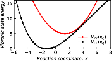
Statistical properties of the bath fluctuations are represented by the Ohmic spectral density function

with parameter $s=3$, cutoff frequency $w_{\mathrm{c}}=0.1$ and the bath reorganization energy $\Lambda_{n}^{\text{bath}}=0.2$ for each $n$. The frequency range of the bath vibrational modes $w\in\left[0.05,\ 2\right]$ was uniformly covered by $40$ modes with discretization step size of $\text{d}w=0.05$. This setup is sufficiently dense to produce the convergent dynamics and the interval of frequencies is wide enough to cover all relevant resonances of the system-bath interactions.

The system and the bath interact via electronic-bath coupling (Eq. 5) and one single vibrational-bath coupling term $k_{nqp}^{\left(1,2\right)}\hat{x}_{q}\hat{\chi}_{p}^{2}$ (see Eq. 6). I.e., for simplicity we set scaling factors to $\gamma^{\left(1,2\right)}=1$ and $\gamma^{\left(1,1\right)}=\gamma^{\left(2,1\right)}=0$. Condition $\gamma^{\left(1,1\right)}=0$ guarantees that the bath vibrational modes are retained as the normal modes, while $\gamma^{\left(2,1\right)}=0$ implies that the double vibrational quanta absorption by the system is not included.

Initial condition of the system and the bath are taken to correspond to the lowest energy states. Assuming that either transition $|0\rangle\rightarrow|1\rangle$ is optically forbidden or is off-resonant, the optical excitation by an external field is modeled using the Franck-Condon ground $|0\rangle$ to excited $|2\rangle$ state electronic transition. This corresponds to the projection of the system ground state wavepacket into the 2-nd excited state potential surface, setting $\varPhi_{2}\left(x,0\right)=\frac{1}{\sqrt{2\pi}}e^{-\frac{x^{2}}{2}}$ and $\varPhi_{1}\left(x,0\right)=0$. Wavepackets of the bath are Gaussian as well, and they can be exactly represented by a single CS. Correspondingly, we choose to set initial amplitudes to $\theta_{1}\left(0\right)=1$, $\theta_{2\ldots M}\left(0\right)=0$ and CS displacements to $\lambda_{\alpha p}\left(0\right)=0$ for every combination of $\alpha,p$ indices: at $t=0$ there are $M$ degenerate CSs, while only the first $\alpha=1$ CS amplitude is non-zero, and all QHO wavepackets are centered in their respective coordinate-momentum phase space $\left(\chi_{p}=0,\rho_{p}=0\right)$. Notice, that when $M>1$, the same bath initial condition can be achieved by parametrizing coherent states differently, we will look at it later in this work.

In summary, the presented theory allows to investigate non-reversible molecular internal conversion dynamics with simultaneous system thermal energy dissipation to the bath. We defined $\text{sD}_{2}$ ansatz, which represents the most essential states for internal conversion, i.e., entangled electron-vibrational wavepacket states, formally exactly, while bath quantum harmonic oscillator states were expanded in a superposition of coherent states. To have thermal energy dissipation to the bath, we included non-linear coupling term $\hat{H}_{\text{V-B}}\propto\hat{x}_{q}\hat{\chi}_{p}^{2}$ between the system and the bath vibrational modes. Using non-adiabatically coupled three-site model, we showed that non-linear system-bath coupling induced non-reversible internal conversion requires highly non-Gaussian bath quantum harmonic oscillator wavepacket representation, as well as, that non-linear coupling results in a broadened and asymmetrically squeezed wavepacket. We argue that these effects are, per definition, not possible to model with simple Davydov $\text{D}_{2}$ ansatz, while squeezed coherent state representation is insufficient. Also, that coupling terms linearly proportional to bath vibrational mode coordinate $\hat{H}\propto\hat{\chi}_{p}$ does not induce wavepacket changes, thus, bath state representation by a single coherent state is sufficient. Additionally, we compared model dynamics and convergence with degenerate and non-degenerate initial coherent states and found that the degenerate case provided the same convergent result as the non-degenerate situation, however, required less computational effort. The presented approach is general and could be used to model effects of other types of non-linear system-bath couplings.

This research was funded by the European Social Fund under the No 09.3.3-LMT-K-712 “Development of Competences of Scientists, other Researchers and Students through Practical Research Activities” measure. T. M. was supported by the Czech Science Foundation (GACR) grant no. 17-22160S. Computations were performed on resources at the High Performance Computing Center „HPC Sauletekis“ in Vilnius University Faculty of Physics.

There are no conflicts of interest to declare.

References

- (1) Balevičius, V, Abramavicius, D, Polívka, T, Galestian Pour, A, & Hauer, J. (2016) J. Phys. Chem. Lett. 7, 3347–3352.
- (2) Balevičius Jr, V, Wei, T, Di Tommaso, D, Abramavicius, D, Hauer, J, Polívka, T, & Duffy, C. D. P. (2019) Chem. Sci. 10, 4792–4804.
- (3) Meneghin, E, Volpato, A, Cupellini, L, Bolzonello, L, Jurinovich, S, Mascoli, V, Carbonera, D, Mennucci, B, & Collini, E. (2018) Nat. Commun. 9, 3160.
- (4) Staleva-Musto, H, West, R, Trathnigg, M, Bína, D, Litvín, R, & Polívka, T. (2019) Faraday Discuss. 216, 460–475.
- (5) Thyrhaug, E, Lincoln, C. N, Branchi, F, Cerullo, G, Perlík, V, Šanda, F, Lokstein, H, & Hauer, J. (2018) Photosynth. Res. 135, 45–54.
- (6) Fox, K. F, Balevičius, V, Chmeliov, J, Valkunas, L, Ruban, A. V, & Duffy, C. D. P. (2017) Phys. Chem. Chem. Phys. 19, 22957–22968.
- (7) Malý, P, Gruber, J. M, Cogdell, R. J, Mančal, T, & van Grondelle, R. (2016) Proc. Natl. Acad. Sci. U. S. A. 113, 2934–9.
- (8) Valkunas, L, Abramavicius, D, & Mančal, T. (2013) Molecular Excitation Dynamics and Relaxation. (Wiley-VCH).
- (9) Weiss, U. (2012) Quantum Dissipative Systems. (WORLD SCIENTIFIC).
- (10) Breuer, H.-P & Petruccione, F. F. (2002) The Theory of Open Quantum Systems. (Oxford University Press), p. 625.
- (11) Tanimura, Y & Kubo, R. (1989) J. Phys. Soc. Japan 58, 101–114.
- (12) Tanimura, Y. (1990) Phys. Rev. A 41, 6676–6687.
- (13) Kreisbeck, C & Kramer, T. (2012) J. Phys. Chem. Lett. 3, 2828–2833.
- (14) Balevičius, V, Gelzinis, A, Abramavicius, D, & Valkunas, L. (2013) J. Phys. Chem. B 117, 11031–11041.
- (15) Redfield, A. G. (1957) IBM J. Res. Dev. 1, 19–31.
- (16) Redfield, A. G. (1965) in Adv. Magn. Opt. Reson. Vol. 1, pp. 1–32.
- (17) Förster, T. (1948) Ann. Phys. 437, 55–75.
- (18) May, V & Kühn, O. (2011) Charge and Energy Transfer Dynamics in Molecular Systems: Third Edition. (Wiley-VCH).
- (19) Dinh, T.-C & Renger, T. (2016) J. Chem. Phys. 145, 034105.
- (20) Seibt, J & Mančal, T. (2017) J. Chem. Phys. 146, 174109.
- (21) Lindblad, G. (1976) Commun. Math. Phys. 48, 119–130.
- (22) Meyer, H.-D, Manthe, U, & Cederbaum, L. (1990) Chem. Phys. Lett. 165, 73–78.
- (23) Beck, M, Jäckle, A, Worth, G, & Meyer, H.-D. (2000) Phys. Rep. 324, 1–105.
- (24) Wang, H & Thoss, M. (2003) J. Chem. Phys. 119, 1289–1299.
- (25) Wang, H & Thoss, M. (2008) New J. Phys. 10, 115005.
- (26) Ronto, M & Shalashilin, D. V. (2013) J. Phys. Chem. A 117, 6948–6959.
- (27) Richings, G, Polyak, I, Spinlove, K, Worth, G, Burghardt, I, & Lasorne, B. (2015) Int. Rev. Phys. Chem. 34, 269–308.
- (28) Shalashilin, D. V & Child, M. S. (2000) J. Chem. Phys. 113, 10028–10036.
- (29) Shalashilin, D. V & Child, M. S. (2004) J. Chem. Phys. 121, 3563–3568.
- (30) Shalashilin, D. V. (2010) J. Chem. Phys. 132, 244111.
- (31) Makhov, D. V, Symonds, C, Fernandez-Alberti, S, & Shalashilin, D. V. (2017) Chem. Phys. 493, 200–218.
- (32) Worth, G. A & Burghardt, I. (2003) Chem. Phys. Lett. 368, 502–508.
- (33) Worth, G, Robb, M, & Lasorne, B. (2008) Mol. Phys. 106, 2077–2091.
- (34) Weiss, S, Eckel, J, Thorwart, M, & Egger, R. (2008) Phys. Rev. B 77, 195316.
- (35) Thorwart, M, Eckel, J, Reina, J, Nalbach, P, & Weiss, S. (2009) Chem. Phys. Lett. 478, 234–237.
- (36) Davydov, A. S. (1979) Phys. Scr. 20, 387–394.
- (37) Scott, A. C. (1991) Phys. D Nonlinear Phenom. 51, 333–342.
- (38) Somoza, A. D, Sun, K.-W, Molina, R. A, & Zhao, Y. (2017) Phys. Chem. Chem. Phys. 19, 25996–26013.
- (39) Werther, M & Grossmann, F. (2018) Phys. Scr. 93, 074001.
- (40) Zhou, N, Huang, Z, Zhu, J, Chernyak, V, & Zhao, Y. (2015) J. Chem. Phys. 143, 014113.
- (41) Zhou, N, Chen, L, Huang, Z, Sun, K, Tanimura, Y, & Zhao, Y. (2016) J. Phys. Chem. A 120, 1562–1576.
- (42) Wang, L, Chen, L, Zhou, N, & Zhao, Y. (2016) J. Chem. Phys. 144, 024101.
- (43) Chorošajev, V, Gelzinis, A, Valkunas, L, & Abramavicius, D. (2014) J. Chem. Phys. 140, 244108.
- (44) Huynh, T. D, Sun, K.-W, Gelin, M, & Zhao, Y. (2013) J. Chem. Phys. 139, 104103.
- (45) Chen, L, Gelin, M. F, Domcke, W, & Zhao, Y. (2015) J. Chem. Phys. 142, 164106.
- (46) Chen, L, Gelin, M. F, & Domcke, W. (2019) J. Chem. Phys. 150, 024101.
- (47) Domcke, W, Yarkony, D. R, & Köppel, H. (2004) Conical Intersections: Electronic Structure, Dynamics & Spectroscopy. (WORLD SCIENTIFIC).
- (48) Jakučionis, M, Chorošajev, V, & Abramavičius, D. (2018) Chem. Phys. 515, 193–202.
- (49) Frenkel, J. (1931) Phys. Rev. 37, 17–44.
- (50) Rodney, L. (2000) The Quantum Theory of Light. (OUP Oxford).
- (51) Shipman, L. L, Cotton, T. M, Norris, J. R, & Katz, J. J. (1976) J. Am. Chem. Soc. 98, 8222–8230.
- (52) Kosumi, D, Fujiwara, M, Fujii, R, Cogdell, R. J, Hashimoto, H, & Yoshizawa, M. (2009) J. Chem. Phys. 130, 214506.
- (53) Chorošajev, V, Marčiulionis, T, & Abramavicius, D. (2017) J. Chem. Phys. 147, 074114.
- (54) Abramavičius, D & Marčiulionis, T. (2018) Lith. J. Phys. 58, 307–317.
- (55) Worth, G. A, Meyer, H.-D, & Cederbaum, L. S. (1998) J. Chem. Phys. 109, 3518–3529.
- (56) Sala, M, Guérin, S, & Gatti, F. (2015) Phys. Chem. Chem. Phys. 17, 29518–29530.
- (57) Chorošajev, V, Rancova, O, & Abramavicius, D. (2016) Phys. Chem. Chem. Phys. 18, 7966–7977.
- (58) Wang, L, Fujihashi, Y, Chen, L, & Zhao, Y. (2017) J. Chem. Phys. 146, 124127.