Uncertainty Visualization of 2D Morse Complex Ensembles Using Statistical Summary Maps
Abstract
Morse complexes are gradient-based topological descriptors with close connections to Morse theory. They are widely applicable in scientific visualization as they serve as important abstractions for gaining insights into the topology of scalar fields. Noise inherent to scalar field data due to acquisitions and processing, however, limits our understanding of the Morse complexes as structural abstractions. We, therefore, explore uncertainty visualization of an ensemble of 2D Morse complexes that arises from scalar fields coupled with data uncertainty. We propose statistical summary maps as new entities for capturing structural variations and visualizing positional uncertainties of Morse complexes in ensembles. Specifically, we introduce two types of statistical summary maps – the Probabilistic Map and the Survival Map – to characterize the uncertain behaviors of local extrema and local gradient flows, respectively. We demonstrate the utility of our proposed approach using synthetic and real-world datasets.
Index Terms:
Morse complexes, uncertainty visualization, topological data analysisI Introduction
Understanding the effects of data uncertainty on visualizations is one of the top research challenges [1, 2, 3, 4]. Uncertainty in visualizations cannot be averted due to noise inherent to data acquisitions, approximations during data processing, and the limitations of rendering devices [2]. The visualization of uncertainty can potentially improve our ability to reason about visualized data [5]. A common practice to mitigate the effects of uncertainty is to combine multiple simulations of a phenomenon (e.g., with varying parameters and different instruments) into an ensemble dataset; see [6] for a survey on ensemble visualization.

In this paper, we investigate the uncertainty in Morse complexes, an important type of topological descriptor, for an ensemble of 2D scalar fields. Morse complexes and Morse-Smale complexes are topological descriptors based on Morse theory [7, 8] that provide abstract representations of the gradient flow behavior of scalar fields [9, 10]. Morse-Smale complexes have shown great utility in numerous scientific applications, from identifying burning regions in combustion experiments [11] to counting bubbles in mixing fluids [12]. They also appear in partition-based regression [13, 14] and statistical inference [15].
Morse complexes [16] are the building blocks for Morse-Smale complexes. Given a Morse function defined on a manifold , , the Morse complex of decomposes the domain into cells, referred to as descending manifolds, where points in the same cell have their gradient flows terminate at the same local maximum. The Morse complex of decomposes the domain into cells, referred to as ascending manifolds, where points in the same cell have their gradient flows originate from the same local minimum. If the ascending and descending manifolds intersect transversally, the set of intersections creates the Morse-Smale complex of , which partitions the domain into cells with uniform gradient behavior. Fig. 1 illustrates the Morse and Morse-Smale complexes of a 2D height function . In particular, for the Morse complex in Fig. 1a, -cells are the critical points of (red for local maxima, blue for local minima, and green for saddles), -cells are integral lines (in white) connecting the critical points, and -cells are connected regions in the domain separated by -cells (see Sec. III for details).
Morse and Morse-Smale complexes have been extensively studied under both piecewise-linear (PL) and combinatorial settings (see Sec. II). However, visualization of Morse and Morse-Smale complexes in the face of uncertainty remains challenging. By uncertainty we mean information about their accuracy, confidence, and variability [1]. In terms of accuracy, Gyulassy et al. [17] have introduced algorithms that improve upon the geometric quality of Morse-Smale complexes. Their algorithms are shown to produce the correct results on average, and the standard deviation approaches zero with increasing mesh resolution. In terms of variability, Thompson et al. [18] have briefly mentioned a Monte Carlo sampling method to quantify variations in the boundaries of Morse complexes.
Motivated by limited prior work in encoding uncertainty of topological descriptors [19, 20], we study the uncertainty in Morse complexes for an ensemble of 2D scalar fields under a particular noise model. Suppose ensemble members are given as scalar functions defined on a shared 2D domain, , where . We study an ensemble of Morse complexes computed from these functions. We assume that each ensemble member is drawn from a distribution that is concentrated around a ground truth function , i.e., for any . The specific models of noise can be quite general (parametric or nonparametric), but we assume to be upper bounded by half of the persistence of the smallest topological feature of the ground truth function (see Sec. III, Sec. IV, and Sec. VII for details).
In this work, we propose statistical summary maps as new entities for visualizing structural variations of Morse complexes. Such structural variations encompass positional uncertainties of -cells of an ensemble of Morse complexes that arises from a common domain and a ground truth function . We introduce two types of statistical summary maps, the Probabilistic Map, (where is the number of local maxima of ), and the Survival Map, , to be utilized in uncertainty visualization.
Overview. We begin with an overview of our computational pipeline for deriving statistical summary maps, as illustrated in Fig. 2.

Given an ensemble of 2D scalar fields, we compute an ensemble of Morse complexes . For our first approach, we study positional uncertainties of local maxima across the ensemble to derive a Probabilistic Map. We first extract (clusters of) mandatory local maxima across the ensemble using techniques developed by David et al. [21]. Specifically, we demonstrate that mandatory local maxima have a one-to-one correspondence with the local maxima of the ground truth function under our noise model (Fig. 2b and Sec. VII). We assign a label to each mandatory local maxima (and, equivalently, to each local maxima of ); let denote the set of labels. Second, for each point in the domain, we compute a probability distribution of its cluster membership across the ensemble. That is, fix an ensemble member , we trace the ascending integral line of each point toward its destination, a local maximum , and assign to the label of as its cluster membership; let denote such an assignment. The Probabilistic Map is defined as a discrete probability distribution of for each . We visualize the Probabilistic Map using color blending in Fig. 2c, where each color represents a distinct label of a mandatory local maximum; see Sec. IV for details.
For our second approach, we quantify structural deviations in local gradient flows across the ensemble via a Survival Map. Specifically, we study directional changes of gradient flows as a result of persistence simplification [22]. For a fixed ensemble member , we first apply a hierarchical persistence simplification (Fig. 2d) of using persistence as a scale parameter. We assign a survival measure for each point based on how frequently it changes its local gradient flows during the simplification process. The less frequently changes its gradient directions, the greater is its survival measure, and vice versa. In other words, the survival measure quantifies the survivability of consistent flow behaviors. Let denote such an assignment of the survival measure. The Survival Map is defined to be the average value of survival measures across the ensemble for each ; that is, . We visualize the Survival Map using a heat color map (blue means low and yellow means high survivability value); see Sec. V for details.
Contribution. In summary, given a 2D Morse complex ensemble:
- •
We exploit mandatory local maxima [21] that capture positional uncertainties among local maxima across the ensemble to derive a Probabilistic Map.
- •
We employ information obtained during persistence simplification [22] of each ensemble member that characterizes structural variations among local gradient flows to derive a Survival Map.
- •
We apply various uncertainty visualization techniques, such as interactive probability queries [23], to our Probabilistic Map and Survival Map for understanding the Morse-complex structural uncertainty in synthetic and real-world datasets.
II Related Work
Representations of Morse-Smale Complexes. Morse and Morse-Smale complexes are defined for functions on smooth -manifolds. Moving from the smooth category to the discrete category requires considerable effort to ensure structural integrity and to simulate differentiability [16]. In general, Morse-Smale complexes can be represented explicitly or implicitly [24]. The first, an explicit representation, is computed in 2D [16] and 3D [25] for piecewise linear (PL) functions defined on triangulated domains. The -skeleton (-cells and -cells) of a Morse-Smale complex is represented as a graph, referred to as the Morse-Smale graph, which connects critical points (as nodes) with separatrices (as edges). The second, an implicit representation, originates from Discrete Morse theory [26, 27, 28, 29] where a Morse-Smale complex is implicitly represented by a combinatorial gradient field [24]. The simplification of Morse-Smale complexes works differently depending on their representations; see [24] for a detailed investigation. Many algorithmic efforts have focused on practical and efficient computations using either of these representations (e.g., [30, 31, 32]). We present our results for the explicit representations of Morse complexes, although our methods do not depend upon the choice of the representation. Note that in image analysis, the watershed algorithm [33] is analogous to the computation of Morse complexes in low dimensions.
Uncertainty visualization of critical points and gradient fields. For a scalar function, its critical points and induced gradient field characterize the structure of its corresponding Morse complex. A few recent works have focused on data uncertainty and its effects on the critical points and gradient fields. Mihai and Westermann [34] have proposed likelihood visualizations of the critical points for an uncertain scalar field. Hüttenberger et al. [35] have exploited the idea of Pareto optimality for predicting the positions of local extrema for multifield data. Günther et al. [21] have devised mandatory critical regions as a way to segment the domain of uncertain data, where at least one critical point of an unknown underlying function is guaranteed to exist within a mandatory critical region. Favelier et al. [36] have developed persistence-based clustering of ensemble members followed by mandatory critical regions for visualizing positional uncertainties of critical points. In this work, we leverage the idea of mandatory critical regions in our Probabilistic Map (Sec. IV).
Pfaffelmoser et al. [37] have analyzed the variability in gradient fields induced by uncertain scalar fields; where gradients are computed using the notion of central differences. Otto et al. [38, 39] have proposed Monte Carlo gradient sampling for visualizing variations of pathlines in 2D and 3D uncertain vector fields. Bhatia et al. [40] have studied the edge maps for error analysis of uncertain gradient flows. Nagraj et al. [41] have proposed a measure to quantify gradient uncertainty for multifield data.
Uncertainty visualization of topological descriptors. A major challenge in visualizing topological descriptors is to encode data uncertainty. Various uncertainty visualization techniques [42, 43, 44] have been proposed to explore structural variations of contour trees for noisy data. Recent work by Lin et al. [20] is the first to study structural averages of merge trees in the context of uncertainty visualization. The analysis and visualization of topological variations in the context of uncertain data remains an open research challenge [19].
III Technical Background
Morse complexes. We focus on the construction of 2D Morse complexes. For simplicity, let be a 2D smooth manifold with boundary (we further ignore the boundary condition for most of our discussion). Let be a Morse function; denotes its gradient. A point is considered critical if ; otherwise it is regular. At any regular point , the gradient is well defined, and integrating it in both ascending and descending directions traces out an integral line, which is a maximal path whose tangent vectors agree with the gradient [55]. Each integral line begins and ends at critical points. The descending manifold surrounding a local maximum is defined as all the points whose integral lines end at the local maximum. The descending manifolds decompose the domain into -cells, whereas critical points are the -cells, and integral lines connecting the critical points are tfhe -cells. As illustrated in Fig. 1(a), these cells form a complex called a Morse complex of , denoted as (whenever is clear from the context). In particular, all the points inside a single -cell have their local gradient flows (integral lines) ending at the same local maximum.
Similarly, the ascending manifold surrounding a local minimum is defined as all the points whose integral lines begin at the local minimum. The ascending manifolds decompose the domain into a dual complex called the Morse complex of (Fig. 1(b)), where points in the same -cell have their integral lines originating from the same local minimum. The set of intersections of ascending and descending manifolds creates the Morse-Smale complex of (Fig. 1(c)) .
Persistence and persistence simplification. Persistent homology is a tool in topological data analysis for quantifying the significance of topological features. We give a 1D illustrative example of persistence below; see [56] for an introduction.

To study the scalar field topology of a 1D Morse function (where ), we focus on the topological structures of its sublevel sets. The sublevel sets of are defined as for any . The D persistent homology tracks the connected components (D topological features) of sublevel sets as increases from . Let be the function values of critical points , respectively. The collection of sublevel sets forms a filtration connected by inclusion maps. Treating as a time parameter, as increases, components of appear and disappear when passes through critical values.
As illustrated in Fig. 3, a 1D function within its visible domain contains six critical points: local minima are in blue and local maxima are in red. As increases from , a component is born (appears) at time when the sublevel set passes through a local minimum . Such a component is represented by the critical point that gives birth to it. Similarly, a second component is born at and represented by ; a third component is born at and represented by . At , the component represented by and the component represented by merge into one component. For consistency, the younger component represented by (the one that is born later) dies (disappears) as a result of the merge. In other words, gives rise to a component that is destroyed by . The critical points and therefore form a persistence pair . With an abuse of notation, we attach a persistence measure to the critical points and that captures the lifespan or significance (called persistence) of the topological feature they represent, i.e., their function value difference, . The birth time and the death time of such a component also give rise to a point in the persistence diagram on the plane. Similarly, the component that is born at dies at , and the component that is born at dies at , giving rise to two more points and in the persistence diagram.
Persistence introduces the notion of scale for learning the structure of a function where small-scale features are commonly considered as noise. Therefore, it is widely used for topological de-noising through persistence simplification [22]. As illustrated in Fig. 3, the critical point pair with the smallest persistence can be simplified producing a simplified function.
In visualization, persistence has been used to simplify topological structures, such as Morse and Morse-Smale complexes [16, 57]. The concept of persistence computation in 1D illustrated in Fig. 3 can be extended to high-dimensional functions. For a 2D scalar function, we create a hierarchical Morse complex [22] by simplifying persistence pairs (in this case, maximum-saddle pairs) in the order of increasing persistence values [24]. Persistence assigned to each critical point in the complex intuitively describes the scale at which a critical point disappears through simplification. Persistence pairs can be simplified by successively canceling pairs of critical points connected in the complex with minimal persistence while avoiding certain degenerate situations (see [24] for implementational details). Fig. 4 illustrates the process of persistence simplification for a 2D Morse complex. A saddle-maximum pair with the minimal persistence in Fig. 4a is simplified in Fig. 4c. The simplification merges two 2D Morse complex cells into one; the blue cell represented by local maximum merges into the red cell represented by local maximum . The (ascending) integral lines of all points in the blue cell change their destination from to . We leverage changes in flow directions in the derivation of the Survival Map (Sec. V).

IV Probabilistic Map
For our first approach, we introduce a Probabilistic Map that utilizes positional uncertainties of local maxima across ensemble members to derive structural uncertainty in a Morse complex. Following an overview in Sec. I, we describe our pipeline via a synthetic dataset, called the Ackley dataset.

Fig. 5a visualizes the Ackley function [58] as the ground truth. is made into a Morse function using simulation of simplicity [59]. contains nine local maxima, which produces nine 2-cells in its corresponding Morse complex in Fig. 5b. Let be the persistence of the smallest (-cells) topological feature in . We generate an ensemble of uncertain scalar fields by mixing with noise sampled from a uniform distribution ; an ensemble member is shown in Fig. 5c. For comparison, we compute the mean field of the ensemble, and visualize its Morse complex in Fig. 5d. The Morse complex of appears similar to the ground truth; however, it does not capture structural variations on the boundaries of Morse complex cells.
Computing the Probabilistic Map. First, we compute mandatory maxima for an ensemble of uncertain Ackley functions , resulting in mandatory local maxima; see Fig. 6a. Under our noise model (see Sec. VII for details), the number of mandatory maxima is consistent with the number of local maxima in the ground truth function . We assign a label to each mandatory local maxima (and equivalently, to each local maxima of ); let denote the set of labels. In Fig. 6a, the labels of mandatory maxima are represented by different colors.

Second, we apply persistence simplification to the Morse complex [24] of each until we are left with local maxima for each ensemble member. We then cluster local maxima (obtained after simplification) across all ensemble members into clusters; see Fig. 6b.
Third, for each point in the domain, we compute a probability distribution of its cluster membership across the ensemble. That is, fix an ensemble member that arises from , we trace the ascending integral line of each point toward its destination, a local maximum , and assign to the label of as its cluster membership; let denote such an assignment.

Finally, the Probabilistic Map is defined to be a discrete probability distribution of label assignments for each . Each is assigned labels across ensemble members. Let be the number of times is assigned a label divided by . Then . For a point , if (implying for all ) for some , then is a point with certainty; otherwise it is a point with uncertainty. Points with certainty are those whose gradient flows to the same mandatory local maximum across ensemble members. Points with uncertainty are those whose flow behaviors vary across ensemble members.
Visualizing the Probabilistic Map. Fig. 7a visualizes for the Ackley dataset. Fig. 7b shows the points with certainty in color; for example, all points in the orange region have their gradients flow to the same mandatory local maximum. The white regions are points with uncertainty. Points with uncertainty are further visualized in Fig. 7c based on their proximity to the points with certainty; for example, the orange points in Fig. 7c are the points that have higher probabilities of flowing to the orange cluster shown in Fig. 6b than the other nearby clusters. For a pair of adjacent regions with different labels and (e.g., orange vs. light green), a black contour contains all points such that for some cluster label ; we refer to such black contours as the expected boundaries.
We employ color blending to visualize . Let be the coloring function. Suppose each mandatory local maximum is assigned a color, , where . is the probability of a point having its gradient flow terminate in a mandatory local maximum with the label . Point is then assigned a color .

Interactive Queries. To further understand the points with uncertainty in (Fig. 7a), we provide interactive queries based on the framework of Potter et al. [23], which focuses on interactive visualization of probability and cumulative density functions. Fig. 8 illustrates such interactive queries for a Probabilistic Map of the Ackley dataset for four point locations with uncertainty. As illustrated by the bar charts, both points and are dominantly orange, while point is mainly violet and orange, and point is primarily red and orange. Interactive queries not only shed light on flow uncertainties but also enable us to adjust cluster membership for an ensemble.

Probabilistic Map for Nonparametric Distributions. We compare the Probabilistic Map vs. the Morse complex of the mean field in Fig. 9 for nonparametric, multimodal noise distributions. The regions with uncertainty in are overlaid with the Morse complex boundaries computed from the ground truth (green), the mean field (red), and the points with (black). The black (expected) boundaries from the Probabilistic Map lie closer to the ground truth than the red boundaries from the mean field. The Probabilistic Map, therefore, not only captures positional variations but also provides reasonable approximations of Morse complex cell boundaries.
V Survival Map
For our second approach, we introduce a Survival Map to quantify structural deviations in local gradient flows across ensemble members (see Fig. 2d). Instead of studying the spatial correlations among local maxima, we study directional changes of gradient flows as a result of persistence simplification [22, 24].
For each ensemble member that arises from a function , we apply a hierarchical persistence simplification (Fig. 2d) of . In the case of a Morse complex, we focus on canceling maximum-saddle pairs until only the global maximum remains. We introduce a survival measure for each point based on how frequently it changes its local gradient flows during the simplification process; let denote such an assignment. Let denote the persistence of maximum-saddle pairs to be cancelled in increasing order, where is the total number of local maxima in . We now describe our algorithm in detail.
First, we compute for each ensemble member. We initialize to be zero everywhere. We perform steps of persistence simplification. For each step (), we cancel the maximum-saddle pair with the lowest persistence value (see Fig. 4). As a result, the gradient flows surrounding the local maximum are redirected to a nearby local maxima , effectively merging the -cell sounding into the -cell surrounding . For all points in the -cell surrounding , we increase by . Intuitively, is incremented within a local neighborhood of where the gradient flow directions survive (remain unchanged) after persistence simplification. The above process is repeated until , i.e., when the entire Morse complex is simplified into a single -cell surrounding the global maximum.
Fig. 4 illustrates one step of our algorithm with a toy example. Suppose we simplify the maximum-saddle pair with the lowest persistence ; this means that the blue 2-cell merges into the red 2-cell after persistence simplification. is increased by for all points in the red 2-cell of Fig. 4a, and it is unchanged everywhere else in the domain. therefore captures the survivability of local gradient flows after persistence simplification.
Second, the Survival Map is computed as the average value of survival measures across the ensemble for each , that is, . Fig. 10 shows the Survival Map of the Ackley dataset using heat color map. The yellow region suggests the existence of a relatively tall peak, and the dark blue regions represent the existence of relatively low peaks across all ensemble members. This behavior is consistent with the ground truth Ackley function depicted in Fig. 5a.

Quantized visualization. To gain insight into the variability of -cells as boundaries of the -cells in the Survival Map, we employ a quantized visualization to further differentiate the regions with uncertainty. In particular, we divide the range of into a fixed number of intervals and visualize the pre-image of each interval using a miscellaneous color map. For example, as shown in Fig. 10(b), the regions with higher color fluctuations indicate positions with higher uncertainty in gradient flow directions.
VI Results
We demonstrate the utility of our proposed statistical summary maps for gaining insights into Morse complex uncertainty for synthetic and real-world datasets.
VI-A Himmelblau’s Function Dataset
Fig. 11 visualizes the Morse complexes for the Himmelblau’s function dataset [60]. The Himmelblau’s function is a multi-modal function containing four local maxima with equal heights; see Fig. 11a; for our purpose, it is perturbed to be a Morse function using simulation of simplicity [59]. We generate an ensemble of functions from with noise , and visualize the Morse complex of the mean field (Fig. 11c). The -cells in the Morse complex of the mean field have distorted boundaries in comparison with the ground truth (Fig. 11b), and they do not give any insight into the positional uncertainties of such boundaries.

The Probabilistic Map and interactive queries at four locations are illustrated in Fig. 12. The Survival Map visualized in Fig. 13a has three colored regions. The orange and green regions in the ground truth (Fig. 11b) are perceived as a single yellow region in Fig. 13a, which contains local maxima with similar heights across ensemble members. The fuzzy regions in Fig. 13a give insight into the flow uncertainty within the ensemble. A quantized visualization of in Fig. 13b further highlights the flow variations in regions with uncertainty. Note that the survival measures attain a narrower range (from to ) for the Himmelblau’s functions compared to the ones for the Ackely function (Fig. 10a). In Fig. 13c, the black contours represent the expected boundaries for the Probabilistic Map visualized in Fig. 12.


VI-B Kármán Vortex Street Dataset
In our first real-world example, we work with the Kármán Vortex Street ensemble dataset. The original flow simulation of Kármán Vortex Street is available via the Gerris software [61]; it is generated as a result of a steady flow (moving from left to right) obstructed by an obstacle situated at the far left. We generate an ensemble of scalar fields representing uncertainty in flow velocity by perturbing the uncertain fluid viscosity parameter. Each ensemble member is computed as the magnitude of the flow velocity after perturbation. We first compute the mean field of the ensemble, as illustrated in Fig. 14a. Yellow regions indicate vortical structures in the flow. The Morse complexes of the mean field before and after persistence simplification are shown in Fig. 14b and Fig. 14c, respectively.

Even though persistence simplification (Fig. 14c) of the mean field gives rise to fewer -cells and a high-level view of its gradient behavior, it does not capture positional uncertainties of the 2-cell boundaries. Fig. 15 visualizes Morse complexes of two ensemble members. The positional variations of 2-cell boundaries appear to be substantial, even after persistence simplification.


We first compute the Probabilistic Map for the Kármán Vortex Street ensemble dataset. Fig. 16a visualizes mandatory local maxima of the ensemble, which form clusters. Each cluster is assigned a unique color. Based on our noise model, we simplify the Morse complex for each ensemble member until local maxima are left. For each ensemble member after simplification, we overlay its local maxima (hollow circles) with the mandatory local maxima (colored regions) in Fig. 16a. The dotted blue boxes enclose locations where local maxima for all ensemble members are contained within mandatory maxima clusters; whereas the dotted pink boxes enclose locations where local maxima for a few ensemble members are not contained in any mandatory maxima clusters (see Sec. VII for details). We assign labels (colors) to the (hollow) local maxima based on the labeling of their nearest mandatory local maxima in Fig. 16b.

Having identified mandatory maximum clusters, we compute the cluster membership probabilities for each position and visualize the probabilities through color blending; see Fig. 17a for the Probabilistic Map. Fig. 18 visualizes interactive queries of in the regions with uncertainty at eight query locations to gain a quick insight into uncertainty surrounding those locations. The red contours in Fig. 19 visualize the spatial inconsistency of 2-cell boundaries of the mean-field Morse complex with the expected boundaries represented by the black contours.
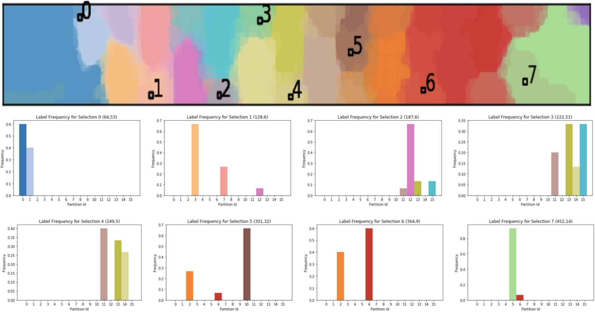


For uncertainty-aware exploration of ensemble members, we further study the positional uncertainty among 2-cells by changing the agreement threshold . As illustrated in Fig. 20 top, the 2-cells visualized at threshold represent the points that flow to a single mandatory maximum among at least of ensemble members. For instance, the points contained in a magenta 2-cell flow to a magenta cluster (Fig. 16b) in at least of the ensemble members. For , the region enclosed by the dotted box (Fig. 20 middle) highlights the positional uncertainty as a mixture of green and red mandatory maxima. The query selection of region for the same region in Fig. 18 shows that the gradient flows toward the green and red clusters (Fig. 16b) in and of ensemble members, respectively.

Finally, we visualize the Survival Map (Fig. 21a). The 2-cells with different shades of yellow, green, and blue indicate the presence of relatively high, moderate, and low local maxima, respectively, across all ensemble members. The quantized visualization in Fig. 21b offers a further insight: the 2-cells with relatively large color fluctuations indicate the positional uncertainty in their boundaries.
VI-C Weather Dataset
In our second real-world example, we analyze an ensemble of vector fields with members that is part of a climate dataset11 1 https://iridl.ldeo.columbia.edu/. Fig. 22a shows the mean vector field with color encoding vector magnitudes. Fig. 22b and Fig. 22c visualize the Morse complex 2-cells before and after persistence simplification of the mean field, respectively. Fig. 23 shows the Morse complexes for two ensemble members. Their 2-cell boundaries are shown to vary substantially before and after persistence simplification.


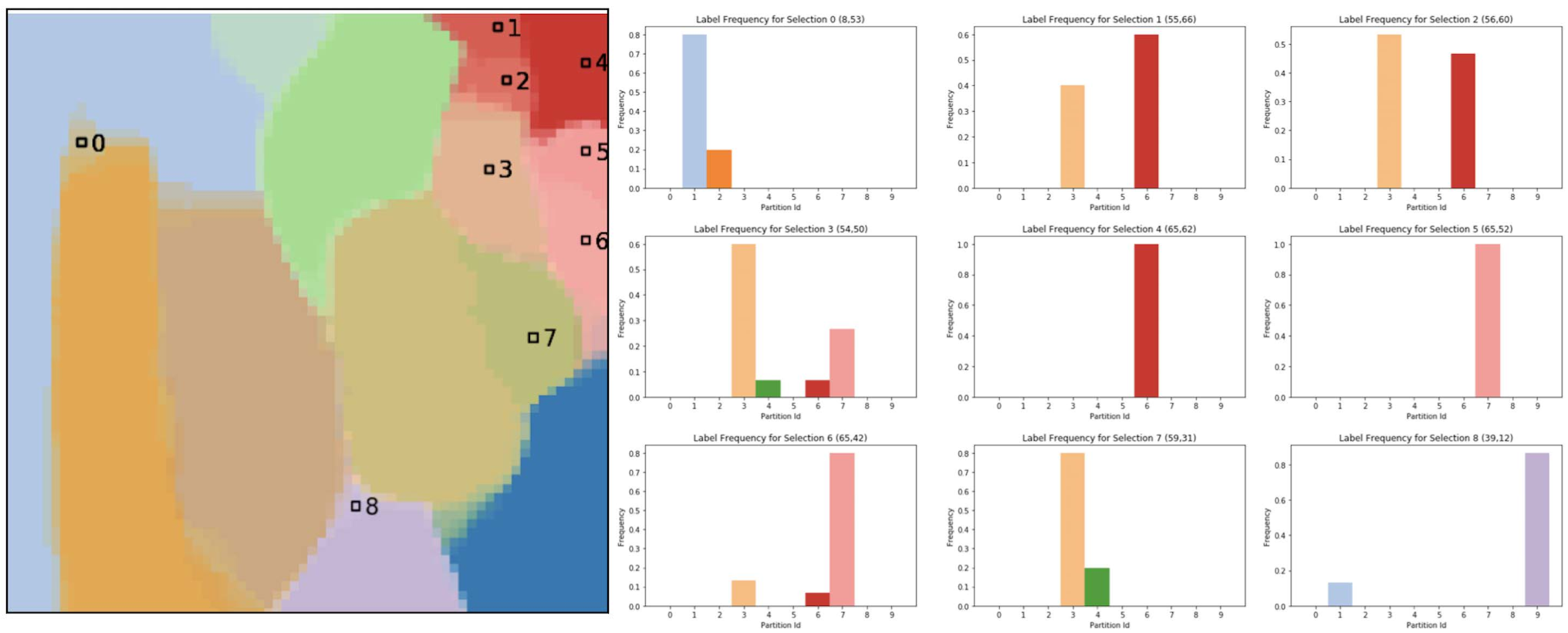
We first explore the Probabilistic Map in Fig. 24a, which visualizes 10 unique mandatory local maxima of the ensemble. Based on our noise model, we simplify the Morse complex for each ensemble member until local maxima are left. For each ensemble member after simplification, we overlay its local maxima (hollow circles) with the mandatory local maxima (colored regions) in Fig. 24a. We assign labels (colors) to the (hollow) local maxima based on the labeling of their nearest mandatory local maxima in Fig. 24b. We compute the cluster membership probabilities for each domain position and visualize the probabilities through color blending in Fig. 25.


Fig. 26 further visualizes interactive queries of in the regions with uncertainty. The positional uncertainty among the 2-cells is explored by changing the agreement threshold for ensemble members, as shown in Fig. 27.

Finally, we compute and visualize the Survival Map in Fig. 28a, which gives insight into the relative heights of local maxima encoded by the survival measure. The quantized visualization in Fig. 28b gives further insight into the 2-cells of the Morse complex, similarly to the setting of the Kármán vortex street dataset.

VII Noise Model
We justify our noise model with respect to mandatory local maxima [21]. Specifically, we demonstrate by experiments that mandatory local maxima have a one-to-one correspondence with the local maxima of the ground truth function under our noise model.
Suppose ensemble members are given as scalar functions defined on a shared 2D domain, , where . We study an ensemble of Morse complexes computed from these functions. We assume that each ensemble member is drawn from a distribution that is concentrated around a ground truth function , i.e., for any . Let denote the persistence of the smallest topological feature of the ground truth function . We assume .
For simplicity, for a fixed ensemble member , we assume we have uniform noise , and let and ; we have for all . Let represents the persistence diagram of the sublevel set filtration of . Based on the stability of the persistence diagrams [62], . However, the stability of critical values is not the same as the stability of critical points; therefore, we need additional machinery. Using the stability of critical points with interval persistence [63], we can show that under our noise model, there is no pairing switches among the critical points; therefore, there is a one-to-one correspondence between the mandatory local maxima and the local maxima of the ground truth function.

We demonstrate the above one-to-one correspondence via a synthetic dataset that arises from a mixture of four Gaussians, . We compute for the ground truth function . Three synthetic ensemble datasets are then generated with three noise levels, , , and . The mandatory maxima are computed for each ensemble. In all cases with , we obtain the same number (four) of mandatory local maxima as the number of local maxima in the ground truth. Fig. 29 illustrates the result for one such experiment; the visualization is generated using the topology toolkit [64]. For , we also get clear separation among mandatory local maxima. With , the mandatory maxima start expanding and eventually merge with one another.
Violation of our noise model. One-to-one correspondence (between mandatory critical points and critical points of all ensemble members) may not be preserved for certain ensemble members that do not conform to our noise model (i.e., ), we would need to employ heuristics to deal with such cases; this include computing the nearest mandatory maxima and clustering of local maxima. For the real-world datasets (Sec. VI-B and Sec. VI-C), we implement the nearest mandatory maximum heuristics (Fig. 16 and Fig. 24) to derive the Probabilistic Map. The clustering of local maxima is illustrated in Fig. 30a for deriving the Probabilistic Map (Fig. 30b) under a noise level .

Furthermore, for quantized visualization, the color fluctuations spatially grow in size with increase in the noise level (that violates our noise model), as illustrated in Fig. 31.

VIII Conclusion and Future Work
We study Morse complexes for ensembles representing uncertain 2D scalar data. We propose statistical summary maps as new abstractions for quantifying structural variations among ensembles of Morse complexes. We introduce two types of statistical summary maps, the Probabilistic Map and the Survival Map . The Probabilistic Map takes advantage of mandatory maxima [21] whereas the Survival Map leverages local gradient flows based on persistence simplification [22]. We employ uncertainty visualization methods such as color mapping, interactive distribution queries, and uncertainty-aware exploration to understand the structural variability captured by our statistical summary maps.
For future work, we plan to generalize our noise model. We also would like to extend our work for Morse complexes beyond 2D. While Morse complexes may be approximated in higher dimensions, visualizing positional uncertainties in higher dimensions will require new visual mappings.
Acknowledgments
This project is supported in part by NSF IIS-1513616, DBI-1661375, and IIS-1910733; National Institute of General Medical Sciences of NIH under grant P41 GM103545-18; and the Intel Parallel Computing Centers Program.
References
- [1] G. Bonneau, H. Hege, C. R. Johnson, M. Oliveira, K. Potter, and P. Rheingans, “Overview and state-of-the-art of uncertainty visualization,” in Scientific Visualization: Uncertainty, Multifield, Biomedical, and Scalable Visualization, M. Chen, H. Hagen, C. Hansen, C. R. Johnson, and A. Kauffman, Eds. Springer, 2014, pp. 5–30.
- [2] K. Brodlie, R. O. Allendes, and A. Lopes, “A review of uncertainty in data visualization,” Expanding the Frontiers of Visual Analytics and Visualization, pp. 81–109, 2012.
- [3] C. R. Johnson and A. R. Sanderson, “A next step: Visualizing errors and uncertainty,” IEEE Computer Graphics and Applications, vol. 23, no. 5, pp. 6–10, 2003.
- [4] K. Potter, J. Kniss, R. Riesenfeld, and C. R. Johnson, “Visualizing summary statistics and uncertainty,” Computer Graphics Forum, vol. 29, no. 3, pp. 823–831, 2010.
- [5] J. Hullman, X. Qiao, M. Correll, A. Kale, and M. Kay, “In pursuit of error: A survey of uncertainty visualization evaluation,” IEEE Transactions on Visualization and Computer Graphics, vol. 25, no. 1, pp. 903–913, 2019.
- [6] J. Wang, S. Hazarika, C. Li, and H.-W. Shen, “Visualization and visual analysis of ensemble data: A survey,” IEEE Transactions on Visualization and Computer Graphics, 2018.
- [7] M. Morse, “Relations between the critical points of a real function of n independent variables,” Transactions of the American Mathematical Society, vol. 27, pp. 345–396, 1925.
- [8] J. Milnor, Morse Theory. New Jersey, NY, USA: Princeton University Press, 1963.
- [9] S. Smale, “On gradient dynamical systems,” Annals of Mathematics Second Series, vol. 74, pp. 199–206, 1961.
- [10] ——, “Generalized poincaré’s conjecture in dimensions greater than four,” Annals of Mathematics Second Series, vol. 74, pp. 391–406, 1961.
- [11] P.-T. Bremer, G. Weber, V. Pascucci, M. Day, and J. Bell, “Analyzing and tracking burning structures in lean premixed hydrogen flames,” IEEE Transactions on Visualization and Computer Graphics, vol. 16, no. 2, pp. 248–260, 2010.
- [12] D. Laney, P.-T. Bremer, A. Mascarenhas, P. Miller, and V. Pascucci, “Understanding the structure of the turbulent mixing layer in hydrodynamic instabilities.” IEEE Transactions on Visualization and Computer Graphics, vol. 12, no. 5, pp. 1052–1060, 2006.
- [13] S. Gerber, O. Rübel, P.-T. Bremer, V. Pascucci, and R. T. Whitaker, “Morse-smale regression,” Journal of Computational and Graphical Statistics, pp. 193–214, 2012.
- [14] D. Maljovec, B. Wang, P. Rosen, A. Alfonsi, G. Pastore, C. Rabiti, and V. Pascucci, “Rethinking sensitivity analysis of nuclear simulations with topology,” IEEE Pacific Visualization Symposium, 2016.
- [15] Y.-C. Chen, C. R. Genovese, and L. Wasserman, “Statistical inference using the Morse-Smale complex,” Electronic Journal of Statistics, vol. 11, no. 1, pp. 1390–1433, 2017.
- [16] H. Edelsbrunner, J. Harer, and A. J. Zomorodian, “Hierarchical Morse-Smale complexes for piecewise linear 2-manifolds,” Discrete and Computational Geometry, vol. 30, pp. 87–107, 2003.
- [17] A. Gyulassy, P.-T. Bremer, and V. Pascucci, “Computing Morse-Smale complexes with accurate geometry,” IEEE Transactions on Visualization and Computer Graphics, vol. 18, no. 12, pp. 2014–2022, 2012.
- [18] D. Thompson, J. A. Levine, J. C. Bennett, P.-T. Bremer, A. Gyulassy, and V. Pascucci, “Analysis of large-scale scalar data using hixels,” IEEE Symposium on Large Data Analysis and Visualization, 2011.
- [19] C. Heine, H. Leitte, M. Hlawitschka, F. Iuricich, L. De Floriani, G. Scheuermann, H. Hagen, and C. Garth, “A survey of topology-based methods in visualization,” Computer Graphics Forum, vol. 35, no. 3, pp. 643–667, 2016.
- [20] L. Yan, Y. Wang, E. Munch, E. Gasparovic, and B. Wang, “A structural average of labeled merge trees for uncertainty visualization,” IEEE Transactions on Visualization and Computer Graphics, vol. 26, no. 1, pp. 832 – 842, 2020.
- [21] G. David, S. Joseph, and T. Julien, “Mandatory critical points of 2D uncertain scalar fields,” Computer Graphics Forum, vol. 33, no. 3, pp. 31–40, 2014.
- [22] H. Edelsbrunner, D. Letscher, and A. J. Zomorodian, “Topological persistence and simplification,” Discrete and Computational Geometry, vol. 28, pp. 511–533, 2002.
- [23] K. Potter, M. Kirby, D. Xiu, and C. R. Johnson, “Interactive visualization of probability and cumulative density functions,” International Journal for Uncertainty Quantification, vol. 2, no. 4, pp. 397–412, 2012.
- [24] D. Günther, J. Reininghaus, H.-P. Seidel, and T. Weinkauf, “Notes on the simplification of the Morse-Smale complex,” in Topological Methods in Data Analysis and Visualization III, P.-T. Bremer, I. Hotz, V. Pascucci, and R. Peikert, Eds. Springer International Publishing, 2014, pp. 135–150.
- [25] H. Edelsbrunner, J. Harer, V. Natarajan, and V. Pascucci, “Morse-Smale complexes for piecewise linear 3-manifolds,” Proceedings of the 19th ACM Symposium on Computational Geometry, pp. 361–370, 2003.
- [26] R. Forman, “Morse theory for cell complexes,” Advances in Mathematics, vol. 134, pp. 90–145, 1998.
- [27] ——, “Combinatorial vector fields and dynamical systems,” Mathematische Zeitschrift, vol. 228, no. 4, pp. 629–681, 1998.
- [28] ——, “Combinatorial differential topology and geometry,” New Perspectives in Geometric Combinatorics, vol. 38, 1999.
- [29] ——, “A user’s guide to discrete Morse theory,” Séminaire Lotharingien de Combinatoire, vol. 48, 2002.
- [30] A. Gyulassy, V. Natarajan, V. Pascucci, and B. Hamann, “Efficient computation of Morse-Smale complexes for three-dimensional scalar functions,” IEEE Transactions on Visualization and Computer Graphics, vol. 13, pp. 1440–1447, 2007.
- [31] A. Gyulassy, P.-T. Bremer, V. Pascucci, and B. Hamann, “A practical approach to Morse-Smale complex computation: Scalability and generality,” IEEE Transactions on Visualization and Computer Graphics, vol. 14, no. 6, pp. 1619–1626, 2008.
- [32] J. Reininghaus, C. Lowen, and I. Hotz, “Fast combinatorial vector field topology,” IEEE Transactions on Visualization and Computer Graphics, vol. 14, no. 6, pp. 1433–1443, 2011.
- [33] S. Beucher and F. Meyer, “The morphological approach to segmentation: the watershed transformation,” Mathematical Morphology in Image Processing, pp. 433–481, 1993.
- [34] M. Mihai and R. Westermann, “Visualizing the stability of critical points in uncertain scalar fields,” Computers and Graphics, vol. 41, pp. 13 – 25, 2014.
- [35] L. Huettenberger, C. Heine, H. Carr, G. Scheuermann, and C. Garth, “Towards multifield scalar topology based on pareto optimality,” Computer Graphics Forum, vol. 32, no. 3, pp. 341–350, 2013.
- [36] G. Favelier, N. Faraj, B. Summa, and J. Tierny, “Persistence atlas for critical point variability in ensembles,” IEEE Transactions on Visualization and Computer Graphics, vol. 25, no. 1, pp. 1152–1162, 2019.
- [37] T. Pfaffelmoser, M. Mihai, and R. Westermann, “Visualizing the variability of gradients in uncertain 2D scalar fields,” IEEE Transactions on Visualization and Computer Graphics, vol. 19, no. 11, pp. 1948–1961, 2013.
- [38] M. Otto, T. Germer, H.-C. Hege, and H. Theisel, “Uncertain 2D vector field topology,” Computer Graphics Forum, vol. 29, no. 2, pp. 347–356, 2010.
- [39] M. Otto, T. Germer, and H. Theisel, “Uncertain topology of 3D vector fields,” in IEEE Pacific Visualization Symposium, 2011, pp. 67–74.
- [40] H. Bhatia, S. Jadhav, P. Bremer, G. Chen, J. Levine, L. Nonato, and V. Pascucci, “Flow visualization with quantified spatial and temporal errors using edge maps.” IEEE Transactions on Visualization and Computer Graphics, vol. 18, no. 9, pp. 1383–1396, 2012.
- [41] S. Nagaraj, V. Natarajan, and R. S. Nanjundiah, “A gradient-based comparison measure for visual analysis of multi-field data reconstruction of gradient in volume rendering,” Eurographics/IEEE Symposium on Visualization, vol. 30, no. 3, 2011.
- [42] M. Kraus, “Visualization of uncertain contour trees,” Proceedings of the International Conference on Information Visualization Theory and Applications, pp. 132–139, 2010.
- [43] K. Wu and S. Zhang, “A contour tree based visualization for exploring data with uncertainty,” International Journal for Uncertainty Quantification, vol. 3, no. 3, pp. 203–223, 2012.
- [44] W. Zhang, P. K. Agarwal, and S. Mukherjee, “Contour trees of uncertain terrains,” Proceedings of the 23rd SIGSPATIAL International Conference on Advances in Geographic Information Systems, vol. 43, 2015.
- [45] R. Whitaker, M. Mirzargar, and R. Kirby, “Contour boxplots: A method for characterizing uncertainty in feature sets from simulation ensembles,” IEEE Transactions on Visualization and Computer Graphics, vol. 19, no. 12, pp. 2713–2722, 2013.
- [46] K. Pöthkow, B. Weber, and H.-C. Hege, “Probabilistic marching cubes,” Computer Graphics Forum, vol. 30, no. 3, pp. 931–940, 2011.
- [47] K. Pöthkow and H.-C. Hege, “Nonparametric models for uncertainty visualization,” Computer Graphics Forum, vol. 32, no. 3.2, pp. 131–140, 2013.
- [48] T. Athawale and A. Entezari, “Uncertainty quantification in linear interpolation for isosurface extraction,” IEEE Transactions on VIsualization and Computer Graphics, vol. 19, no. 12, pp. 2723–2732, 2013.
- [49] T. Athawale, E. Sakhaee, and A. Entezari, “Isosurface visualization of data with nonparametric models for uncertainty,” IEEE Transactions on VIsualization and Computer Graphics, vol. 19, no. 12, pp. 2723–2732, 2016.
- [50] T. Athawale and C. R. Johnson, “Probabilistic asymptotic decider for topological ambiguity resolution in level-set extraction for uncertain 2d data,” IEEE Transactions on Visualization and Computer Graphics, vol. 25, no. 1, pp. 1163–1172, 2019.
- [51] I. Demir, C. Dick, and R. Westermann, “Multi-charts for comparative 3d ensemble visualization,” IEEE Transactions on Visualization and Computer Graphics, vol. 20, no. 12, pp. 2694–2703, 2014.
- [52] J. Weissenbock, B. Frohler, E. Groller, J. Kastner, and C. Heinzl, “Dynamic volume lines: Visual comparison of 3D volumes through space-filling curves,” IEEE Transactions on Visualization and Computer Graphics, vol. 25, no. 1, pp. 1040–1049, 2019.
- [53] S. Liu, J. Levine, P.-T. Bremer, and V. Pascucci, “Gaussian mixture model based volume visualization,” in Proceedings of the IEEE Large-Scale Data Analysis and Visualization Symposium, 2012, pp. 73–77.
- [54] E. Sakhaee and A. Entezari, “A statistical direct volume rendering framework for visualization of uncertain data,” IEEE Transactions on VIsualization and Computer Graphics, vol. 23, no. 12, pp. 2509–2520, 2017.
- [55] H. Edelsbrunner, J. Harer, and A. Zomorodian, “Hierarchical Morse complexes for piecewise linear 2-manifolds,” in Proceedings 17th Annual Symposium on Computational Geometry, 2001, pp. 70–79.
- [56] H. Edelsbrunner and J. Harer, “Persistent homology - a survey,” Contemporary Mathematics, vol. 453, pp. 257–282, 2008.
- [57] A. Gyulassy and V. Natarajan, “Topology-based simplification for feature extraction from 3d scalar fields,” in Proceedings IEEE Visualization, 2005, pp. 535–542.
- [58] D. H. Ackley, A connectionist machine for genetic hillclimbing. Kluwer Academic Publishers Norwell, MA, USA, 1987.
- [59] H. Edelsbrunner and E. P. Mücke, “Simulation of simplicity: A technique to cope with degenerate cases in geometric algorithms,” ACM Transactions on Graphics, vol. 9, pp. 66–104, 1990.
- [60] D. Himmelblau, Applied Nonlinear Programming. McGraw-Hill, 1972.
- [61] S. Popine, “Gerris: A tree-based adaptive solver for the incompressible euler equations in complex geometries,” Journal of Computational Physics, vol. 190, no. 2, pp. 572–600, 2003.
- [62] D. Cohen-Steiner, H. Edelsbrunner, and J. Harer, “Stability of persistence diagrams,” Discrete and Computational Geometry, vol. 37, pp. 103–120, 2007.
- [63] T. Dey and R. Wenger, “Stability of critical points with interval persistence,” Discrete & Computational Geometry, vol. 38, pp. 479–512, 2007.
- [64] J. Tierny, G. Favelier, J. A. Levine, C. Gueunet, and M. Michaux, “The topology toolkit,” IEEE Transactions on Visualization and Computer Graphics, no. 1, pp. 832 – 842, Jan 2018.