跳到论文正文
W Papers独立论文阅读器 arXiv:1912.06296 论文正文 计算阅读时间 · 0%
引用这篇论文根据当前论文元数据生成,正式投稿前建议核对。


License: arXiv.org perpetual non-exclusive license
arXiv:1912.06296v1 [math.OC] 13 Dec 2019

On Privatizing Equilibrium Computation in Aggregate Games over NetworksThis work is partially supported by a Siebel Energy Institute Grant and the Joan and Lalit Bahl Fellowship at Illinois.

Shripad Gade   Anna Winnicki   Subhonmesh Bose Address: Department of Electrical and Computer Engineering, University of Illinois at Urbana-Champaign, Urbana, IL 61801.
{gade3, annaw5, boses}@illinois.edu
Abstract

We propose a distributed algorithm to compute an equilibrium in aggregate games where players communicate over a fixed undirected network. Our algorithm exploits correlated perturbation to obfuscate information shared over the network. We prove that our algorithm does not reveal private information of players to an honest-but-curious adversary who monitors several nodes in the network. In contrast with differential privacy based algorithms, our method does not sacrifice accuracy of equilibrium computation to provide privacy guarantees.

keywords
Privacy, Nash Equilibrium Computation, Networked Aggregate Games.

1 Introduction

Aggregate games are non-cooperative games in which a player’s payoff or cost depends on her own actions and the sum-total of the actions taken by other players. In a Cournot oligopoly for example, firms compete to supply a product in a market with a price-responsive demand with a goal to maximize profit. A firm’s profit depends on her production cost as well as the market price, where the latter only depends on the aggregate quantity of the product offered in the market by all firms. Aggregate games are widely studied in the literature, e.g., see Novshek 1985; Jensen 2010. Multiple strategic interactions in practice admit an aggregate game model, e.g., Cournot competition models for wholesale electricity markets in Willems et al. 2009; Cai et al. 2019; Cherukuri and Cortés 2019, supply function competition in general economies see Jensen 2010, communication networks in Teng et al. 2019; Koskie and Gajic 2005 and common agency games in Martimort and Stole 2011. Aggregate games are often potential games and a pure-strategy Nash equilibrium can be guaranteed to exist. In this paper, we present an algorithm for networked players to compute such an equilibrium in a distributed fashion that maintains the privacy of players’ cost structures.

Players in a networked game can only communicate with neighboring players in a communication graph. Distributed algorithms for computing Nash equilibrium in networked games have a rich literature, e.g., see Koshal et al. 2016; Salehisadaghiani and Pavel 2018; Ye and Hu 2017; Tatarenko et al. 2018; Parise et al. 2015. The obvious difficulty in computing equilibrium strategy arises due to the inability of a player to observe the aggregate decision. Naturally distributed Nash computation proceeds via iterative estimation of the aggregate decision followed by local payoff maximization (or cost minimization) with a given aggregate estimate. Koshal et al. 2016; Parise et al. 2015 exploits consensus based averaging, Koshal et al. 2016; Salehisadaghiani and Pavel 2018 explore gossip based averaging, and Tatarenko et al. 2018 employs gradient play along with acceleration for aggregate estimation over networks.

1.1 Our Contributions

Algorithms for equilibrium computation were not designed with privacy in mind. We show in Section 2.5, that an honest-but-curious adversary can compromise a few nodes in the network and observe the sequence of estimates to infer other players’ payoff or cost structures for the algorithm in Koshal et al. 2016. In other words, information that allows distributed equilibrium computation can leak players’ sensitive private information to adversaries.

Distributed equilibrium computation algorithms require aggregate estimates to update their own actions. Our proposed algorithm obfuscates local aggregate estimates before sharing them with neighbors. The obfuscation step involves players adding correlated perturbations to each outgoing aggregate estimate. The perturbations are designed such that they add to zero for each player. The received perturbed aggregate estimates are averaged by each player and used for updating strategy using local projected gradient descent.

Our main result (Theorem 1) reveals that obfuscation via correlated perturbations prevents an adversary from accurately learning cost structures provided the network satisfies appropriate connectivity conditions. Players converge to exact Nash equilibrium asymptotically. In other words, we simultaneously achieve both privacy and accuracy in distributed Nash computation in aggregate games. This is in sharp contrast to differentially private algorithms where trade-offs between accuracy and privacy guarantee are fundamental, e.g., see Han et al. 2016.

Simulations in Section 4 validate our results and corroborate our intuition that obfuscation slows down but does not impede the convergence of the algorithm.

2 Equilibrium Computation in Aggregate Games and the Lack of Privacy

We begin by introducing a networked aggregate game. We then present an adversary model and show that prior distributed equilibrium computation algorithms leak private information of players. This exposition motivates the development of privacy-preserving algorithms for equilibrium computation in the next section.

2.1 The Networked Aggregate Game Model

Consider a game with NN players that can communicate over a fixed undirected network with reliable lossless links. Model this communication network by graph 𝔊⁡(𝒱,ℰ)\mathfrak{G}({\mathcal{V}},{\mathcal{E}}), where each node in 𝒱:={1,…,N}{\mathcal{V}}:=\{1,\ldots,N\} denotes a player. Two players ii and jj can communicate with each other if and only if they share an edge in ℰ{\mathcal{E}}, denoted as (i,j)∈ℰ(i,j)\in{\mathcal{E}}. Call 𝒩i{\mathcal{N}}_{i} the set of neighbors of node ii and i∈𝒩ii\in{\mathcal{N}}_{i} by definition.

Player ii can take actions in a convex compact set 𝒳i⊆\Rsetd{\mathcal{X}}_{i}\subseteq\Rset^{d}, where \Rset\Rset denotes the set of real numbers. Define 𝒳¯\overline{{\mathcal{X}}} as the Minkowski (set) sum of 𝒳i{\mathcal{X}}_{i}’s and

x¯≔∑j=1Nxj\overline{x}\coloneqq\sum_{j=1}^{N}x_{j}

as the aggregate action of all players. For convenience, define x¯−i≔∑j≠ixi\overline{x}_{-i}\coloneqq\sum_{j\neq i}x_{i}. We assume that ∩i=1N𝒳i\cap_{i=1}^{N}{\mathcal{X}}_{i} is non-empty. For an action profile (x1,…,xN)(x_{1},\ldots,x_{N}), player ii incurs a cost that takes the form fi​(xi,x¯)≔fi​(xi,xi+x¯−i)f_{i}(x_{i},\overline{x})\coloneqq f_{i}\left(x_{i},x_{i}+\overline{x}_{-i}\right). This defines an aggregate game in that the actions of other players affect player ii only through the sum of actions of all players, x¯\overline{x}.

Each player i∈𝒱i\in{\mathcal{V}} thus seeks to solve

minimizefi​(xi,xi+x¯−i),subject toxi∈𝒳i.\displaystyle\begin{aligned} &\text{minimize}&&f_{i}(x_{i},x_{i}+\overline{x}_{-i}),\\ &\text{subject to}&&x_{i}\in{\mathcal{X}}_{i}.\end{aligned} (1)

For each i∈𝒱i\in{\mathcal{V}}, assume that fi​(xi,y)f_{i}(x_{i},y) is continuously differentiable in (xi,y)(x_{i},y) over a domain that contains 𝒳i×𝒳¯{\mathcal{X}}_{i}\times\overline{{\mathcal{X}}}. Furthermore, for each i∈𝒱i\in{\mathcal{V}}, let xi↦fi​(xi,x¯)x_{i}\mapsto f_{i}(x_{i},\overline{x}) be convex over 𝒳i{\mathcal{X}}_{i} and the gradient ∇xifi\nabla_{x_{i}}f_{i} be uniformly L¯\overline{L}-Lipschitz, i.e., ∃L¯>0\exists\ \overline{L}>0 such that,

‖∇xifi​(xi,u)−∇xifi​(xi,u′)‖≤L¯​‖u−u′‖,\displaystyle\|\nabla_{x_{i}}f_{i}(x_{i},u)-\nabla_{x_{i}}f_{i}(x_{i},u^{\prime})\|\leq\overline{L}\|u-u^{\prime}\|, (2)

for all u,u′u,u^{\prime} in 𝒳¯\overline{{\mathcal{X}}}, xix_{i} in 𝒳i{\mathcal{X}}_{i}. Throughout, ∥⋅∥\|\cdot\| stands for the ℓ2\ell_{2}-norm of its argument. Define 𝒳:=×i=1N𝒳i{\mathcal{X}}:=\times_{i=1}^{N}{{\mathcal{X}}_{i}} and the gradient map

ϕ⁡(x):=(∇x1f1​(x1,x¯)∇xNfN​(xN,x¯))\displaystyle\phi(x):=\begin{pmatrix}\nabla_{x_{1}}f_{1}(x_{1},\overline{x})\\ \vdots\\ \nabla_{x_{N}}f_{N}(x_{N},\overline{x})\end{pmatrix} (3)

for x:=(x1⊺,x2⊺,…,xN⊺)⊺∈𝒳x:=(x_{1}^{\mathchoice{\raisebox{0.75346pt}{$\displaystyle\intercal$}}{\raisebox{0.75346pt}{$\textstyle\intercal$}}{\raisebox{0.75346pt}{$\scriptstyle\intercal$}}{\raisebox{0.75346pt}{$\scriptscriptstyle\intercal$}}},x_{2}^{\mathchoice{\raisebox{0.75346pt}{$\displaystyle\intercal$}}{\raisebox{0.75346pt}{$\textstyle\intercal$}}{\raisebox{0.75346pt}{$\scriptstyle\intercal$}}{\raisebox{0.75346pt}{$\scriptscriptstyle\intercal$}}},\ldots,x_{N}^{\mathchoice{\raisebox{0.75346pt}{$\displaystyle\intercal$}}{\raisebox{0.75346pt}{$\textstyle\intercal$}}{\raisebox{0.75346pt}{$\scriptstyle\intercal$}}{\raisebox{0.75346pt}{$\scriptscriptstyle\intercal$}}})^{\mathchoice{\raisebox{0.75346pt}{$\displaystyle\intercal$}}{\raisebox{0.75346pt}{$\textstyle\intercal$}}{\raisebox{0.75346pt}{$\scriptstyle\intercal$}}{\raisebox{0.75346pt}{$\scriptscriptstyle\intercal$}}}\in{\mathcal{X}}. Assume throughout that ϕ\phi is strictly monotone over 𝒳{\mathcal{X}}, i.e.,

[ϕ⁡(x)−ϕ⁡(x′)]⊺​(x−x′)>0,\displaystyle\left[\phi(x)-\phi(x^{\prime})\right]^{\mathchoice{\raisebox{0.75346pt}{$\displaystyle\intercal$}}{\raisebox{0.75346pt}{$\textstyle\intercal$}}{\raisebox{0.75346pt}{$\scriptstyle\intercal$}}{\raisebox{0.75346pt}{$\scriptscriptstyle\intercal$}}}(x-x^{\prime})>0, (4)

for all x,x′∈𝒳x,x^{\prime}\in{\mathcal{X}} and x≠x′x\neq x^{\prime}. Denote this game in the sequel by 𝗀𝖺𝗆𝖾⁡(𝔊,{fi,𝒳i}i∈𝒱){\sf game}(\mathfrak{G},\{f_{i},{\mathcal{X}}_{i}\}_{i\in{\mathcal{V}}}).

To provide a concrete example, consider the well-studied Nash-Cournot game (see Fudenberg and Tirole 1991) among NN suppliers competing to offer into a market for a single commodity where the price pp varies with demand DD as p⁡(D):=a−b​Dp(D):=a-bD. Supplier ii offers to produce xix_{i} amount of goods within its production capability modeled as 𝒳i⊆\Rset+{\mathcal{X}}_{i}\subseteq\Rset_{+}. Here \Rset+\Rset_{+} denotes the set of nonnegative real numbers. To produce xix_{i}, supplier ii incurs a cost of ci​(xi)c_{i}(x_{i}), where cic_{i} is increasing, convex and differentiable. Each supplier seeks to maximize her profit, or equivalently, minimize her loss. The loss of supplier ii is

fi​(xi,x¯)=ci​(xi)−xi​p​(x¯)=ci​(xi)−xi​(a−b​x¯).f_{i}(x_{i},\overline{x})=c_{i}(x_{i})-x_{i}p(\overline{x})=c_{i}(x_{i})-x_{i}(a-b\overline{x}).

2.2 Equilibrium Definition and Existence

An action profile (x1∗,…​xN∗)(x_{1}^{*},\ldots x_{N}^{*}) defines a Nash equilibrium of 𝗀𝖺𝗆𝖾⁡(𝔊,{fi,𝒳i}i∈𝒱){\sf game}(\mathfrak{G},\{f_{i},{\mathcal{X}}_{i}\}_{i\in{\mathcal{V}}}) in pure strategies, if

fi​(xi∗,xi∗+x¯−i∗)≤fi​(xi,xi+x¯−i∗),f_{i}\left(x_{i}^{*},x_{i}^{*}+\overline{x}_{-i}^{*}\right)\leq f_{i}\left(x_{i},x_{i}+\overline{x}_{-i}^{*}\right),

for all xi∈𝒳ix_{i}\in{\mathcal{X}}_{i} and i∈𝒱i\in{\mathcal{V}}.

The networked aggregate game, as described above, always admits a unique pure strategy Nash equilibrium. See Theorem 2.2.3 in Facchinei and Pang 2007 for details. Given that an equilibrium always exists, prior literature has studied distributed algorithms for players to compute such an equilibrium.

2.3 Prior Algorithms for Distributed Nash Computation

We now describe the distributed algorithm in Koshal et al. 2016 for equilibrium computation of 𝗀𝖺𝗆𝖾⁡(𝔊,{fi,𝒳i}i∈𝒱){\sf game}(\mathfrak{G},\{f_{i},{\mathcal{X}}_{i}\}_{i\in{\mathcal{V}}}). In Section 2.5, we demonstrate that adversarial players can infer private information about cost structures fif_{i}’s from observing a subset of the variables during equilibrium computation using that algorithm. While we only study the algorithm in Koshal et al. 2016, our analysis can be extended to those presented in Salehisadaghiani and Pavel 2018; Ye and Hu 2017; Tatarenko et al. 2018; Parise et al. 2015.

Recall that players in 𝗀𝖺𝗆𝖾⁡(𝔊,{fi,𝒳i}i∈𝒱){\sf game}(\mathfrak{G},\{f_{i},{\mathcal{X}}_{i}\}_{i\in{\mathcal{V}}}) do not have access to the aggregate decision. To allow equilibrium computation, let players at iteration kk maintain estimates of the aggregate decision x¯\overline{x} as v1k,…,vNkv^{k}_{1},\ldots,v^{k}_{N}, initialized as, vi0=xi0v^{0}_{i}=x^{0}_{i} for each player ii. At discrete time steps k≥0k\geq 0, each player transmits her own estimate of the aggregate decision to its neighbors and updates her own action as,

v^ik\displaystyle\widehat{v}^{k}_{i} =∑j=1NWi​j​vjk,\displaystyle=\sum_{j=1}^{N}W_{ij}v^{k}_{j}, (5a)
xik+1\displaystyle x^{k+1}_{i} =proj𝒳i​[xik−αk​∇xifi​(xik,N​v^ik)],\displaystyle=\textrm{proj}_{{\mathcal{X}}_{i}}\left[x^{k}_{i}-\alpha^{k}\nabla_{x_{i}}f_{i}(x^{k}_{i},N\widehat{v}^{k}_{i})\right], (5b)
vik+1\displaystyle v^{k+1}_{i} =v^ik+xik+1−xik.\displaystyle=\widehat{v}^{k}_{i}+x^{k+1}_{i}-x^{k}_{i}. (5c)

Here, proj𝒳i\textrm{proj}_{{\mathcal{X}}_{i}} stands for projection on 𝒳i{\mathcal{X}}_{i}, and αk\alpha^{k} is a common learning rate of all players.

The algorithm has three steps. First, player ii computes a weighted average of the estimates of the aggregate received from its neighbors in (5a), where WW is a symmetric doubly-stochastic weighting matrix. The sparsity pattern of the matrix follows that of graph 𝔊\mathfrak{G}, i.e.,

Wi​j≠0⇔(i,j)∈ℰ.W_{ij}\neq 0\iff(i,j)\in{\mathcal{E}}.

Second, player ii performs a projected gradient update in (5b) utilizing the weighted average of local aggregate decision v^ik\widehat{v}^{k}_{i} in lieu of the true aggregate decision x¯\overline{x}. Finally, she updates her own estimate of aggregate average in (5c) based on her local decision xikx_{i}^{k} and its update xik+1x_{i}^{k+1}.

2.4 Adversary Model and Privacy Definition

Consider an adversary 𝖠{\sf{A}} that compromises the players in 𝒜⊆𝒱{\mathcal{A}}\subseteq{\mathcal{V}}. 𝖠{\sf{A}} is equipped with unbounded storage and computational capabilities, and has access to all information stored, processed locally and communicated to any compromised players at all times. We define adversary model using the information available to 𝖠{\sf{A}}.

  1. (A)

    For a compromised node i∈𝒜i\in{\mathcal{A}}, 𝖠{\sf{A}} knows all local information fif_{i}, xikx_{i}^{k}, vikv_{i}^{k}, v^ik\widehat{v}_{i}^{k} and information received from neighbors of ii i.e., vjkv_{j}^{k} for j∈𝒩ij\in{\mathcal{N}}_{i} at each k≥0k\geq 0.

  2. (B)

    𝖠{\sf{A}} knows the algorithm for equilibrium computation and its parameters {αk}\{\alpha^{k}\} and WW.

  3. (C)

    𝖠{\sf{A}} observes aggregate decision x¯k\overline{x}^{k} at each kk.

What does 𝖠{\sf{A}} seek to infer? The dependency of a player’s cost on her own actions encodes private information. In the Cournot competition example, this dependency is precisely supplier ii’s production cost – information that is business sensitive. 𝖠{\sf{A}} seeks to exploit information sequence observed from compromised players to infer private information of other players. Intuitively, privacy implies inability of 𝖠{\sf{A}} to infer private cost functions.

Denote the set of non-adversarial nodes by 𝒜c≔𝒱∖𝒜{\mathcal{A}}^{c}\coloneqq{\mathcal{V}}\setminus{\mathcal{A}}. Call 𝔊⁡(𝒜c)\mathfrak{G}({\mathcal{A}}^{c}) the restriction of 𝔊\mathfrak{G} to 𝒜c{\mathcal{A}}^{c} obtained by deleting the adversarial nodes. See Figure 1 for an illustration. For this example, 𝖠\sf{A} monitors all variables and parameters pertaining to player 5, but seeks to infer the functions f1,…,f4f_{1},\ldots,f_{4}.

Refer to caption
Figure 1: Illustration of 𝔊\mathfrak{G} and 𝔊⁡(𝒜c)\mathfrak{G}({\mathcal{A}}^{c}). Here, 𝒜={5}{\mathcal{A}}=\{5\} and 𝒜c={1,2,3,4}{\mathcal{A}}^{c}=\{1,2,3,4\}.

Let Π\Pi denote the set of all permutations over all non-adversarial nodes in 𝒜c{\mathcal{A}}^{c}. Define the collection of games

ℱ≔{𝗀𝖺𝗆𝖾⁡(𝔊,{fπ⁡(i),𝒳π⁡(i)}i∈𝒱)|π∈Π}.\displaystyle{\mathcal{F}}\coloneqq\Big\{{\sf game}(\mathfrak{G},\{f_{\pi(i)},{\mathcal{X}}_{\pi(i)}\}_{i\in{\mathcal{V}}})\;\Big|\;\pi\in\Pi\Big\}.

Thus, ℱ{\mathcal{F}} comprises the games where the cost functions and strategy sets of non-adversarial players are permuted. All games in ℱ{\mathcal{F}} have the same aggregate strategy x¯∗\overline{x}^{*} at Nash equilibrium. Next, we utilize ℱ{\mathcal{F}} to define privacy.

Definition 1 (Privacy)

Consider a distributed algorithm to compute the Nash equilibrium of 𝗀𝖺𝗆𝖾⁡(𝔊,{fi,𝒳i}i∈𝒱){\sf game}(\mathfrak{G},\{f_{i},{\mathcal{X}}_{i}\}_{i\in{\mathcal{V}}}). If execution observed by adversary 𝖠{\sf{A}} is consistent with all games in ℱ{\mathcal{F}}, then the algorithm is private.

We define privacy as the inability of 𝖠{\sf{A}} to distinguish between games in ℱ{\mathcal{F}}. Even if 𝖠{\sf{A}} knew all possible costs exactly–which is a tall order–our privacy definition implies that 𝖠{\sf{A}} cannot associate such costs to specific players.

2.5 Privacy Breach in Algorithm (5)

Consider a Cournot competition among 5 players connected according to 𝔊\mathfrak{G} in Figure 1, where 𝖠{\sf{A}} has compromised player 55. Assume that the equilibrium of the game lies in the interior of each player’s strategy set. Recall that 𝖠\sf{A} stores observed information at each kk and processes it to infer private cost information ci​(xi)c_{i}(x_{i}). We argue how 𝖠\sf{A} can compute cost functions c1​(⋅),…,c4​(⋅)c_{1}(\cdot),\ldots,c_{4}(\cdot) up to a constant.

We first show privacy breach for player 4. 𝖠{\sf{A}} observes {v1k,v3k,v4k,v5k}\{v^{k}_{1},v^{k}_{3},v^{k}_{4},v^{k}_{5}\} at each k≥0k\geq 0. 𝖠\sf{A} uses v3kv^{k}_{3}, v4kv^{k}_{4}, v5kv^{k}_{5} and WW to compute v^4k\widehat{v}^{k}_{4} using (5a). Moreover, 𝖠{\sf{A}} uses (5c) to compute,

x4k+1−x4k=v4k+1−v^4k.x^{k+1}_{4}-x^{k}_{4}=v^{k+1}_{4}-\widehat{v}^{k}_{4}.

For large enough kk, the step-size αk\alpha^{k} is small enough to ensure,

proj𝒳i​[xik−αk​∇xifi​(xik,N​v^ik)]≈xik−αk​∇xifi​(xik,N​v^ik).\textrm{proj}_{{\mathcal{X}}_{i}}\left[x^{k}_{i}-\alpha^{k}\nabla_{x_{i}}f_{i}(x^{k}_{i},N\widehat{v}^{k}_{i})\right]\approx x^{k}_{i}-\alpha^{k}\nabla_{x_{i}}f_{i}(x^{k}_{i},N\widehat{v}^{k}_{i}).

At such large kk, 𝖠{\sf{A}} uses (5b) along with (x4k+1−x4k)(x^{k+1}_{4}-x^{k}_{4}) and αk\alpha^{k} to calculate ∇x4f4​(x4k,N​v^4k)\nabla_{x_{4}}f_{4}(x^{k}_{4},N\widehat{v}^{k}_{4}).

𝖠{\sf{A}} uses information about strucutre of loss function i.e. f4​(x4,x¯)=c4​(x4)−x4​(a−b​x¯)f_{4}(x_{4},\overline{x})=c_{4}(x_{4})-x_{4}(a-b\overline{x}), along with ∇x4f4​(x4k,N​v^4k)\nabla_{x_{4}}f_{4}(x^{k}_{4},N\widehat{v}^{k}_{4}), v^4k\widehat{v}^{k}_{4}, x¯k\overline{x}^{k} and game parameters a,ba,b to learn c4′​(x4k)c^{\prime}_{4}(x^{k}_{4}). Several observations of (x4k,c4′​(x4k))(x^{k}_{4},c^{\prime}_{4}(x^{k}_{4})) allows 𝖠{\sf{A}} to learn the private cost c4c_{4} upto a constant.

We showed that privacy breach for player 4, the same analysis can be used for players 1, 2 and 3 with an additional step. 𝖠{\sf{A}} observes x¯k\overline{x}^{k}, which tracks 1N​∑ivik\frac{1}{N}\sum_{i}v^{k}_{i} (Lemma 2 in Koshal et al. 2016). 𝖠{\sf{A}} computes

v2k=N​x¯k−(v1k+v3k+v4k+v5k).v^{k}_{2}=N\overline{x}^{k}-(v^{k}_{1}+v^{k}_{3}+v^{k}_{4}+v^{k}_{5}).

Since {v2k}\{v^{k}_{2}\} is available for each k≥0k\geq 0, 𝖠{\sf{A}} uses same process as above to show privacy breach for players 1, 2 and 3.

For algorithm (5), 𝖠\sf{A} uncovers all private cost functions ci​(⋅)c_{i}(\cdot) for an example aggregate game. Next, we design an algorithm that protects privacy of players’ private information in the sense of Definition 1 against 𝖠{\sf{A}}.

3 Our Algorithm and Its Properties

We propose and analyze Algorithm 1 that computes Nash equilibrium of 𝗀𝖺𝗆𝖾⁡(𝔊,{fi,𝒳i}i∈𝒱){\sf game}(\mathfrak{G},\{f_{i},{\mathcal{X}}_{i}\}_{i\in{\mathcal{V}}}) in a distributed fashion. The main result (Theorem 1) shows that the algorithm asymptotically converges to the equilibrium. Attempts by 𝖠{\sf{A}} to recover each player’s cost structure, however, remain unsuccessful.

The key idea behind our design is the injection of correlated noise perturbations in the exchange of local estimates of the aggregate decision. Different neighbors of player ii receive different estimates of the aggregate decision. The perturbations added by any player ii add to zero. While 𝖠\sf{A} may still infer the true aggregate decision, the protocol does not allow him to correctly infer the players’ iterates or the gradients of their costs with respect to their own actions. Our assumption on network connectivity requires 𝒢⁡(𝒜c){\mathcal{G}}({\mathcal{A}}^{c}) be connected and not be bipartite. Under these conditions 𝖠\sf{A} cannot monitor all outgoing communication channels from any player. We further show that one can design noises in a way that 𝖠\sf{A}’s observations are consistent with all games in ℱ{\mathcal{F}}, making it impossible for him to uncover cost for any specific player.

Throughout, assume that WW is a doubly stochastic that follows the sparsity pattern of 𝔊\mathfrak{G}. Further, assume that all non-diagonal, non-zero entries of WW are identically δ<1N−1\delta<\frac{1}{N-1}.

At each time kk, player ii generates correlated random numbers {ri​jk}\{r^{k}_{ij}\} satisfying ri​ik=0r^{k}_{ii}=0 and ∑j∈𝒩iri​jk=0\sum_{j\in\mathcal{N}_{i}}r^{k}_{ij}=0. Player ii then adds αk​ri​jk\alpha^{k}r^{k}_{ij} to vikv^{k}_{i} to generate vi​jkv^{k}_{ij}, the estimate sent by player ii to player jj, according to (8). Let 𝒓{\bm{r}} denote the collection of rr’s for all players across time. Call 𝒓{\bm{r}} the obfuscation sequence.

Each node ii computes weighted average of received aggregate estimates vj​ikv^{k}_{ji} to construct its own estimate aggregate decision N​v^ikN\widehat{v}^{k}_{i}, following (9). Players perform projected gradient descent using local decision estimate xikx^{k}_{i}, gradient of cost function ∇xifi​(xik,N​v^ik)\nabla_{x_{i}}f_{i}(x^{k}_{i},N\widehat{v}^{k}_{i}), and non-summable, square-summable step size αk\alpha^{k} (see (6)) to arrive at an improved local decision estimate xik+1x^{k+1}_{i} using (10). Players then update their local aggregate estimate using the change in local decision estimate xik+1−xikx^{k+1}_{i}-x^{k}_{i} per (11).

Algorithm 1 Private Distributed Nash Computation
1: Input: Player ii knows fi​(xi,x¯)f_{i}(x_{i},\overline{x}), 𝒳i\mathcal{X}_{i}, and δ\delta. Consider a non-increasing non-negative sequence 𝜶{\bm{\alpha}} that satisfies
∑k=1∞αk=∞​ and ​∑k=1∞[αk]2<∞.\displaystyle\hskip-18.06749pt\sum_{k=1}^{\infty}\alpha^{k}=\infty\text{ and }\sum_{k=1}^{\infty}[\alpha^{k}]^{2}<\infty. (6)
2: Initialize: For i∈𝒱i\in{\mathcal{V}}, v0i=x0i=𝓍∈∩𝒾𝒳𝒾v^{0}_{i}=x^{0}_{i}=\mathpzc{x}\in\cap_{i}{\mathcal{X}}_{i}.
3:
4: For k≥0k\geq 0, players i∈𝒱i\in{\mathcal{V}} execute in parallel:
5:
6: Construct |𝒩i||\mathcal{N}_{i}| random numbers {ri​jk}\{r^{k}_{ij}\}, satisfying
ri​ik=0​ and ​∑j∈𝒩iri​jk=0.\displaystyle r_{ii}^{k}=0\text{ and }\sum_{j\in\mathcal{N}_{i}}r^{k}_{ij}=0. (7)
7: Send obfuscated aggregate estimates vi​jkv^{k}_{ij} to j∈𝒩ij\in{\mathcal{N}}_{i}, where
vi​jk=vik+αk​ri​jk.\displaystyle v^{k}_{ij}=v^{k}_{i}+\alpha^{k}r^{k}_{ij}. (8)
8: Compute weighted average of received estimates vj​ikv^{k}_{ji} as
v^ik=∑j=1NWi​j​vj​ik.\displaystyle\widehat{v}^{k}_{i}=\sum_{j=1}^{N}W_{ij}v^{k}_{ji}. (9)
9: Perform a projected gradient descent step as
xik+1=proj𝒳i​[xik−αk​∇xifi​(xik,N​v^ik)].\displaystyle x^{k+1}_{i}=\textrm{proj}_{\mathcal{X}_{i}}[x^{k}_{i}-\alpha^{k}\nabla_{x_{i}}f_{i}(x^{k}_{i},N\widehat{v}^{k}_{i})]. (10)
10: Update local aggregate estimate as
vik+1=v^ik+xik+1−xik.\displaystyle v^{k+1}_{i}=\widehat{v}^{k}_{i}+x^{k+1}_{i}-x^{k}_{i}. (11)

The properties of our algorithm are summarized in the next result. The proof is included in Section 5.

Theorem 1

Consider a networked aggregate game defined as 𝗀𝖺𝗆𝖾⁡(𝔊,{fi,𝒳i}i∈𝒱){\sf game}(\mathfrak{G},\{f_{i},{\mathcal{X}}_{i}\}_{i\in{\mathcal{V}}}). If 𝔊⁡(𝒜c)\mathfrak{G}({\mathcal{A}}^{c}) is connected and not bipartite, then Algorithm 1 is private. Moreover, if the obfuscation sequence is bounded, then Algorithm 1 asymptotically converges to a Nash equilibrium of the game.

The convergence properties largely mimic that of distributed descent algorithms for equilibrium computation. The locally balanced and bounded nature of the designed noise together with decaying step-sizes ultimately drown the effect of the noise. Computing balanced yet bounded perturbations can be achieved using secure multiparty computation protocols described in Gade and Vaidya 2016; Gade and Vaidya 2018b; Abbe et al. 2012. Our assumption on 𝔊⁡(𝒜c)\mathfrak{G}({\mathcal{A}}^{c}) is such that given two games F,F~F,\tilde{F} from ℱ{\mathcal{F}} and an obfuscation sequence 𝒓{\bm{r}}, we are able to design a different obfuscation sequence 𝒓~{\bm{\tilde{r}}}, such that the execution of FF perturbed with 𝒓{\bm{r}} generates identical observables as F~\tilde{F} perturbed with 𝒓~{\bm{\tilde{r}}}. The connectivity among non-adversarial players in 𝒜c{\mathcal{A}}^{c} is key to the success of our algorithm design. Convergence speed depends on the size of the perturbations. We investigate this link experimentally in Section 4, but leave analytical characterization of this relationship for future work. In what follows, we compare our algorithm and its properties to other protocols for privacy preservation.

3.0.1 Comparison with Differentially Private Algorithms:

Differentially private algorithms for computing Nash equilibrium of potential games have been studied in Dong et al. 2015; Cummings et al. 2015. The algorithm in Dong et al. 2015 executes a differentially private distributed mirror-descent algorithm to optimize the potential function. Experiments reveal that a trade-off arises between accuracy and privacy parameters, i.e., the more privacy one seeks, the less accurate the final output of the algorithm becomes. Such a tradeoff is a hallmark of differentially private algorithms, e.g., see Han et al. 2016. Our algorithm on the other hand does not suffer from that limitation. Notice that our definition of privacy is binary in nature. That is, an algorithm for equilibrium computation can either be private or non-private. We aim to explore properties of our algorithmic architecture with notions of privacy that allow for a degree of privacy and compare them with differentially private algorithms.

3.0.2 Comparison to Cryptographic Methods:

Authors in Lu and Zhu 2015 use secure multiparty computation to compute Nash equilibrium. Such an approach guarantees privacy in an information theoretic sense. This protocol provides privacy guarantees along with accuracy, similar to our algorithmic framework. However, cryptographic protocols are typically computationally expensive for large problems (see Section V in Zhang et al. 2019), and are often difficult to implement in distributed settings.

3.0.3 Comparison to Private Distributed Optimization:

Our earlier work in Gade and Vaidya 2018b has motivated the design of Algorithm 1. While our prior work seeks privacy-preserving distributed protocols to cooperatively solve optimization problems, the current paper focuses on non-cooperative games. Protocols in Gade and Vaidya 2018b advocate use of perturbations that cancel over the network. Such a design is not appropriate for networked games for two reasons. First, players must agree on noise design, a premise that requires cooperation. Second, perturbing local functions fif_{i}’s, even if the changes cancel in aggregate, can alter the equilibrium of the game.

3.0.4 Privacy in Client-Server architecture:

This work considers players communicating over a peer-to-peer network. However, engineered distributed systems often have a client-server architecture. Presence of a central server entity allows for easy aggregate computation. However, privacy is sacrificed if the parameter server is adversarial. We have investigated privacy preservation for distribution optimization in this architecture in Gade and Vaidya 2018a, where, we use multiple central servers instead of one, a subset of which can be adversarial. We believe our algorithm design and analysis in Gade and Vaidya 2018a can be extended to deal with private equilibrium computation for aggregate games in client-server framework.

4 A Numerical Experiment

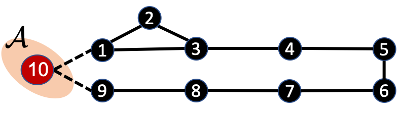
Consider a Cournot competition with N=10N=10 players over 𝔊\mathfrak{G} described in Figure 3. Player ii’s cost is given by

ci​(xi)=ζi,2​xi2+ζi,1​xi.c_{i}(x_{i})=\zeta_{i,2}x_{i}^{2}+\zeta_{i,1}x_{i}.

The cost coefficients are drawn randomly from

ζi,2∼𝗎𝗇𝗂𝖿⁡[0,1/2],ζi,1∼𝗎𝗇𝗂𝖿⁡[0,1]\zeta_{i,2}\sim{\sf unif}[0,1/2],\ \zeta_{i,1}\sim{\sf unif}[0,1]

for each ii. The strategy sets are identically 𝒳i=[0,5]{\mathcal{X}}_{i}=[0,5] for each ii. Choose δ=110\delta=\frac{1}{10} that parameterizes the matrix WW. Let the price vary with demand DD as

p⁡(D)=6−110​D.p(D)=6-\frac{1}{10}D.
Refer to caption
Figure 2: Communication network for Cournot network example on N=10N=10 players.
Figure 3: Iterates generated by Algorithm 1 versus the Algorithm in (5) for Δ={10,20,30,50}\Delta=\{10,20,30,50\}.

We initialize the algorithm with x0=1x^{0}=1 identically for all players. We use secure multi-party computing technique in Gade and Vaidya 2018b to design obfuscation sequence 𝒓{\bm{r}} that satisfies (7) and

|ri​jk|≤Δ.|r_{ij}^{k}|\leq\Delta.

The trajectory of the average distance of xikx^{k}_{i}’s from xi∗x^{*}_{i} across players with αk:=(k+1)0.51\alpha_{k}:=(k+1)^{0.51} is shown in Figure 3.

Our algorithm converges to the equilibrium similar to the non-private algorithm in (5). However, its convergence is slower as seen in Figure 3. The slowdown is especially pronounced for large Δ\Delta’s and is an artifact of perturbations added by players to obfuscate information from the adversary. Thus, our algorithm design achieves privacy and asymptotic convergence to equilibrium, but sacrifices speed of convergence. An analytical characterization of the slowdown defines an interesting direction for future work.

5 Proof of Theorem 1

5.1 Proving Algorithm 1 is Private

Recall that 𝔊⁡(𝒜c)\mathfrak{G}({\mathcal{A}}^{c}) is the graph over non-adversarial nodes 𝒜c{\mathcal{A}}^{c}. Suppose 𝒜c{\mathcal{A}}^{c} has MM nodes. Let I,JI,J be two players in 𝒜c{\mathcal{A}}^{c} and

F:=(fi,𝒳i)i∈𝒱,F~:=(f~i,𝒳~i)i∈𝒱,F:={(f_{i},{\mathcal{X}}_{i})}_{i\in{\mathcal{V}}},\quad\tilde{F}:={(\tilde{f}_{i},\tilde{{\mathcal{X}}}_{i})}_{i\in{\mathcal{V}}},

be two games in ℱ{\mathcal{F}} such that F~\tilde{F} is identical to FF, except that costs and strategy sets of players II and JJ are switched:

f~I=fJ,f~J=fI,𝒳~I=𝒳J,𝒳~J=𝒳I.\tilde{f}_{I}=f_{J},\ \tilde{f}_{J}=f_{I},\ \tilde{{\mathcal{X}}}_{I}={\mathcal{X}}_{J},\ \tilde{{\mathcal{X}}}_{J}={\mathcal{X}}_{I}.

For convenience, define π:𝒱→𝒱\pi:{\mathcal{V}}\to{\mathcal{V}} as the permutation that encodes the switch, i.e.,

π(I)=J,π(J)=I, and π(i)=i for all i≠I,J.\pi(I)=J,\ \pi(J)=I,\text{ and }\pi(i)=i\text{ for all }i\neq I,J.

Consider the execution of Algorithm 1 on FF, given by

𝖤⁡(F,𝒓,𝓍):={(𝓍𝒾𝓀,𝓋𝒾𝓀,𝓋^𝒾𝓀)​ for ​𝒾∈𝒱,𝓀≥0},\displaystyle{\sf{E}}(F,{\bm{r}},\mathpzc{x}):=\{(x^{k}_{i},v^{k}_{i},\widehat{v}^{k}_{i})\text{ for }i\in{\mathcal{V}},k\geq 0\},

with obfuscation sequence 𝒓{\bm{r}} used in (8), initialized with 𝓍∈∩𝒾=1𝒩𝒳𝒾\mathpzc{x}\in\cap_{i=1}^{N}{\mathcal{X}}_{i}. We prove that there exists an obfuscation sequence 𝒓~{\bm{\tilde{r}}} such that execution 𝖤⁡(F~,𝒓~,𝓍){\sf{E}}(\tilde{F},{\bm{\tilde{r}}},\mathpzc{x}) of Algorithm 1 on F~\tilde{F} with 𝒓~{\bm{\tilde{r}}} starting from 𝓍\mathpzc{x}, is identical to 𝖤⁡(F,𝒓,𝓍){\sf{E}}(F,{\bm{r}},\mathpzc{x}), from 𝖠{\sf{A}}’s perspective. An arbitrary permutation over 𝒜c{\mathcal{A}}^{c} is equivalent to a composition of a sequence of switches among two players in 𝒜c{\mathcal{A}}^{c}. As a result, the algorithm execution on games in ℱ{\mathcal{F}} can be made to appear identical from 𝖠{\sf{A}}’s standpoint, proving the privacy of Algorithm 1.

In the rest of the proof, we show how to construct 𝒓~{\bm{\tilde{r}}} that ensures 𝖤⁡(F~,𝒓~,𝓍){\sf{E}}(\tilde{F},{\bm{\tilde{r}}},\mathpzc{x}) and 𝖤⁡(F,𝒓,𝓍){\sf{E}}(F,{\bm{r}},\mathpzc{x}) appear identical to 𝖠{\sf{A}}.

Adversary observes {xjk,vjk,v^jk}\{x^{k}_{j},v^{k}_{j},\widehat{v}^{k}_{j}\} for all j∈𝒜j\in{\mathcal{A}} at each k≥0k\geq 0. Consequently, perturbations utilized by corrupted nodes j∈𝒜j\in{\mathcal{A}} are same in both executions,

r~j​ik=rj​ik​ for all ​j∈𝒜.\displaystyle\tilde{r}^{k}_{ji}=r^{k}_{ji}\text{ for all }j\in{\mathcal{A}}. (12)

Moreover, 𝖠{\sf{A}} observes v^jk\widehat{v}^{k}_{j} for all j∈𝒜j\in{\mathcal{A}} and hence, all messages received by j∈𝒜j\in{\mathcal{A}} from i∈𝒜ci\in{\mathcal{A}}^{c}, denoted by vi​jkv^{k}_{ij}, are identical for both executions, i.e.,

v~i​jk=vi​jk⇔v~ik+αk​r~i​jk=vik+αk​ri​jk⇔αk​r~i​jk=vik+αk​ri​jk−v~ik.\displaystyle\begin{aligned} \tilde{v}^{k}_{ij}={v}^{k}_{ij}&\iff\tilde{v}^{k}_{i}+\alpha^{k}\tilde{r}^{k}_{ij}=v^{k}_{i}+\alpha^{k}r^{k}_{ij}\\ &\iff\alpha^{k}\tilde{r}^{k}_{ij}=v^{k}_{i}+\alpha^{k}r^{k}_{ij}-\tilde{v}^{k}_{i}.\end{aligned} (13)

Adversary observes x¯k\overline{x}^{k} for each k≥0k\geq 0. Enforcing

x~ik=xπ⁡(i)k,v~ik=vπ⁡(i)k,v~^ik=v^π⁡(i)k,\tilde{x}^{k}_{i}=x^{k}_{\pi(i)},\ \tilde{v}^{k}_{i}=v^{k}_{\pi(i)},\ \widehat{\tilde{v}}^{k}_{i}=\widehat{v}^{k}_{\pi(i)},

results in x~¯k=x¯k\overline{\tilde{x}}^{k}=\overline{x}^{k}. We have

v~^ik=v^π⁡(i)k\displaystyle\widehat{\tilde{v}}^{k}_{i}=\widehat{v}^{k}_{\pi(i)}
⇔∑j∈𝒩iWi​j​(v~jk+αk​r~j​ik)=∑j∈𝒩π⁡(i)Wπ⁡(i)​j​(vjk+αk​rj​π​(i)k)\displaystyle\iff\sum_{j\in{\mathcal{N}}_{i}}W_{ij}(\tilde{v}^{k}_{j}+\alpha^{k}\tilde{r}^{k}_{ji})=\sum_{j\in{\mathcal{N}}_{\pi(i)}}W_{\pi(i)j}(v^{k}_{j}+\alpha^{k}r^{k}_{j\pi(i)})
⇔∑j∈𝒩i∩𝒜cr~j​ik=1αk​δ​∑j∈𝒩π⁡(i)Wπ⁡(i)​j​(vjk+αk​rj​π​(i)k)\displaystyle\iff\sum_{j\in{\mathcal{N}}_{i}\cap{\mathcal{A}}^{c}}\tilde{r}^{k}_{ji}=\frac{1}{\alpha^{k}\delta}\sum_{j\in{\mathcal{N}}_{\pi(i)}}W_{\pi(i)j}(v^{k}_{j}+\alpha^{k}r^{k}_{j\pi(i)})
−1αk​δ∑j∈𝒩iWi​jvkπ⁡(j)−∑j∈𝒩i∩𝒜r~kj​i.\displaystyle\qquad\qquad-\frac{1}{\alpha^{k}\delta}\sum_{j\in{\mathcal{N}}_{i}}W_{ij}{v}^{k}_{\pi(j)}-\sum_{j\in{\mathcal{N}}_{i}\cap{\mathcal{A}}}\tilde{r}^{k}_{ji}. (14)

The obfuscation used by each player i∈𝒜ci\in{\mathcal{A}}^{c} is locally balanced, and hence, we have

∑j∈𝒩ir~ki​j=0⇔∑j∈𝒩i∩𝒜cr~ki​j=−∑j∈𝒩i∩𝒜r~ki​j.\displaystyle\sum_{j\in{\mathcal{N}}_{i}}\tilde{r}^{k}_{ij}=0\iff\sum_{j\in{\mathcal{N}}_{i}\cap{\mathcal{A}}^{c}}\tilde{r}^{k}_{ij}=-\sum_{j\in{\mathcal{N}}_{i}\cap{\mathcal{A}}}\tilde{r}^{k}_{ij}. (15)

Let γ\gamma be a vector of r~i​jk\tilde{r}^{k}_{ij}’s for i,j∈𝒜ci,j\in{\mathcal{A}}^{c}. In the sequel, let 𝟙\mathds{1} denote a vector of ones of appropriate dimension. For graph 𝔊⁡(𝒜c)\mathfrak{G}({\mathcal{A}}^{c}), define its oriented incidence matrix BB, adjacency matrix AA, degree matrix DD, and the normalized graph Laplacian matrix LL as

Bi​j={1,if node ​i​ is head of edge ​j,−1,if node ​i​ is tail of edge ​j,0,otherwise,\displaystyle B_{ij}=\begin{cases}1,&\text{if node }i\text{ is head of edge }j,\\ -1,&\text{if node }i\text{ is tail of edge }j,\\ 0,&\text{otherwise},\end{cases}
Ai​j={1,if ​(i,j)​ is edge in ​𝔊​(𝒜c),0,otherwise,\displaystyle A_{ij}=\begin{cases}1,&\text{if }(i,j)\text{ is edge in }\mathfrak{G}({\mathcal{A}}^{c}),\\ 0,&\text{otherwise},\end{cases}
D=diag(A𝟙), and L=I−D−1/2AD−1/2.\displaystyle D=\mathop{\mathrm{diag}}(A\mathds{1}),\text{ and }L=I-D^{-1/2}AD^{-1/2}.

Using the notation z+≔max⁡{z,0}z_{+}\coloneqq\max\{z,0\} and z−≔z+−zz_{-}\coloneqq z_{+}-z for a scalar zz, define B+B_{+} and B−B_{-} as the matrices obtained from BB, applying the respective operator componentwise. Then, (14) - (15) can be written as

(B−B+B+B−)⏟:=Tγ=(ξ1ξ2)⏟:=ξ,\displaystyle\underbrace{\begin{pmatrix}B_{-}&B_{+}\\ B_{+}&B_{-}\end{pmatrix}}_{:=T}\gamma=\underbrace{\begin{pmatrix}\xi^{1}\\ \xi^{2}\end{pmatrix}}_{:=\xi},

We prove that,

rank ​T=rank ​(T|ξ)=2​M−1,\displaystyle\text{rank }T=\text{rank }(T\ |\ \xi)=2M-1, (16)

to show that T​γ=ξT\gamma=\xi admits at least one solution.

Notice that

(𝟙⊺|−𝟙⊺)​(B−B+B+B−)=(−𝟙⊺​B| 1⊺​B)=0,\displaystyle\begin{aligned} (\mathds{1}^{\mathchoice{\raisebox{0.75346pt}{$\displaystyle\intercal$}}{\raisebox{0.75346pt}{$\textstyle\intercal$}}{\raisebox{0.75346pt}{$\scriptstyle\intercal$}}{\raisebox{0.75346pt}{$\scriptscriptstyle\intercal$}}}\ |\ -\mathds{1}^{\mathchoice{\raisebox{0.75346pt}{$\displaystyle\intercal$}}{\raisebox{0.75346pt}{$\textstyle\intercal$}}{\raisebox{0.75346pt}{$\scriptstyle\intercal$}}{\raisebox{0.75346pt}{$\scriptscriptstyle\intercal$}}})\begin{pmatrix}B_{-}&B_{+}\\ B_{+}&B_{-}\end{pmatrix}=\left(-\mathds{1}^{\mathchoice{\raisebox{0.75346pt}{$\displaystyle\intercal$}}{\raisebox{0.75346pt}{$\textstyle\intercal$}}{\raisebox{0.75346pt}{$\scriptstyle\intercal$}}{\raisebox{0.75346pt}{$\scriptscriptstyle\intercal$}}}B\ |\ \mathds{1}^{\mathchoice{\raisebox{0.75346pt}{$\displaystyle\intercal$}}{\raisebox{0.75346pt}{$\textstyle\intercal$}}{\raisebox{0.75346pt}{$\scriptstyle\intercal$}}{\raisebox{0.75346pt}{$\scriptscriptstyle\intercal$}}}B\right)=0,\end{aligned} (17)

proving that rows of TT are not linearly independent. Next, we show that rank ​T≥2​M−1\text{rank }T\geq 2M-1. To that end, we have

rank ​T\displaystyle\text{rank }T =rank ​(T​T⊺)\displaystyle=\text{rank }(TT^{\mathchoice{\raisebox{0.75346pt}{$\displaystyle\intercal$}}{\raisebox{0.75346pt}{$\textstyle\intercal$}}{\raisebox{0.75346pt}{$\scriptstyle\intercal$}}{\raisebox{0.75346pt}{$\scriptscriptstyle\intercal$}}})
=rank ​(B−​B−⊺+B+​B+⊺B−​B+⊺+B+​B−⊺B+​B−⊺+B−​B+⊺B−​B−⊺+B+​B+⊺)\displaystyle=\text{rank }\begin{pmatrix}B_{-}B_{-}^{\mathchoice{\raisebox{0.75346pt}{$\displaystyle\intercal$}}{\raisebox{0.75346pt}{$\textstyle\intercal$}}{\raisebox{0.75346pt}{$\scriptstyle\intercal$}}{\raisebox{0.75346pt}{$\scriptscriptstyle\intercal$}}}+B_{+}B_{+}^{\mathchoice{\raisebox{0.75346pt}{$\displaystyle\intercal$}}{\raisebox{0.75346pt}{$\textstyle\intercal$}}{\raisebox{0.75346pt}{$\scriptstyle\intercal$}}{\raisebox{0.75346pt}{$\scriptscriptstyle\intercal$}}}&\;B_{-}B_{+}^{\mathchoice{\raisebox{0.75346pt}{$\displaystyle\intercal$}}{\raisebox{0.75346pt}{$\textstyle\intercal$}}{\raisebox{0.75346pt}{$\scriptstyle\intercal$}}{\raisebox{0.75346pt}{$\scriptscriptstyle\intercal$}}}+B_{+}B_{-}^{\mathchoice{\raisebox{0.75346pt}{$\displaystyle\intercal$}}{\raisebox{0.75346pt}{$\textstyle\intercal$}}{\raisebox{0.75346pt}{$\scriptstyle\intercal$}}{\raisebox{0.75346pt}{$\scriptscriptstyle\intercal$}}}\\ B_{+}B_{-}^{\mathchoice{\raisebox{0.75346pt}{$\displaystyle\intercal$}}{\raisebox{0.75346pt}{$\textstyle\intercal$}}{\raisebox{0.75346pt}{$\scriptstyle\intercal$}}{\raisebox{0.75346pt}{$\scriptscriptstyle\intercal$}}}+B_{-}B_{+}^{\mathchoice{\raisebox{0.75346pt}{$\displaystyle\intercal$}}{\raisebox{0.75346pt}{$\textstyle\intercal$}}{\raisebox{0.75346pt}{$\scriptstyle\intercal$}}{\raisebox{0.75346pt}{$\scriptscriptstyle\intercal$}}}&\;B_{-}B_{-}^{\mathchoice{\raisebox{0.75346pt}{$\displaystyle\intercal$}}{\raisebox{0.75346pt}{$\textstyle\intercal$}}{\raisebox{0.75346pt}{$\scriptstyle\intercal$}}{\raisebox{0.75346pt}{$\scriptscriptstyle\intercal$}}}+B_{+}B_{+}^{\mathchoice{\raisebox{0.75346pt}{$\displaystyle\intercal$}}{\raisebox{0.75346pt}{$\textstyle\intercal$}}{\raisebox{0.75346pt}{$\scriptstyle\intercal$}}{\raisebox{0.75346pt}{$\scriptscriptstyle\intercal$}}}\end{pmatrix}
=(a)rank ​(DAAD)\displaystyle\stackrel{{\scriptstyle(a)}}{{=}}\text{rank }\begin{pmatrix}D&A\\ A&D\end{pmatrix}
=rank ​D+rank ​(D−A​D−1​A)\displaystyle=\text{rank }D+\text{rank }(D-AD^{-1}A)
=M+rank (IM−D−1/2AD−1AD−1/2)\displaystyle=M+\text{rank }(I_{M}-D^{-1/2}AD^{-1}AD^{-1/2})
=M+rank ​(IM−(IM−L)2)\displaystyle=M+\text{rank }(I_{M}-(I_{M}-L)^{2})
=M+rank ​(2​L−L2)\displaystyle=M+\text{rank }(2L-L^{2})
≥(b)M+rank ​L⏟=M−1+rank ​(2​IM−L)−M\displaystyle\stackrel{{\scriptstyle(b)}}{{\geq}}M+\underbrace{\text{rank }L}_{=M-1}+\text{rank }(2I_{M}-L)-M
=(c)M−1+rank ​(2​IM−L)\displaystyle\stackrel{{\scriptstyle(c)}}{{=}}M-1+\text{rank }(2I_{M}-L)
=2​M−1,\displaystyle=2M-1, (18)

where IMI_{M} is the M×MM\times M identity matrix. Here, (a) follows from the definition of B+,B−,D,AB_{+},B_{-},D,A, (b) follows from Sylvester’s nullity theorem (see Horn and Johnson 2012) and the fact that the rank of graph Laplapcian for the connected graph 𝔊⁡(𝒜c)\mathfrak{G}({\mathcal{A}}^{c}) on MM nodes is M−1M-1. Furthermore, since 𝔊⁡(𝒜c)\mathfrak{G}({\mathcal{A}}^{c}) is not bipartite, the eigenvalues of LL are strictly less than 2, according to Lemma 1.7 in Chung and Graham 1997. Therefore, we have rank ​(2​I−L)=M\text{rank }(2I-L)=M that implies (c). Thus, (17) and (18) together yield rank ​T=2​M−1\text{rank }T=2M-1.

For the augmented matrix (T|ξ)(T\ |\ \xi), we have

2​M−1≤rank ​(T|ξ)≤ 2​M.\displaystyle 2M-1\ \leq\ \text{rank }(T\ |\ \xi)\ \leq\ 2M. (19)

In the above relation, the inequality on the left follows from our earlier proof that rank ​T=2​M−1\text{rank }T=2M-1. The one on the right follows from the fact that the augmented matrix has 2​M2M rows. We demonstrate that rows of (T|ξ)(T\ |\ \xi) are linearly dependent to conclude (16). From (17), we deduce

(𝟙⊺|−𝟙⊺)​(T|ξ)\displaystyle\left(\mathds{1}^{\mathchoice{\raisebox{0.75346pt}{$\displaystyle\intercal$}}{\raisebox{0.75346pt}{$\textstyle\intercal$}}{\raisebox{0.75346pt}{$\scriptstyle\intercal$}}{\raisebox{0.75346pt}{$\scriptscriptstyle\intercal$}}}\ |\ -\mathds{1}^{\mathchoice{\raisebox{0.75346pt}{$\displaystyle\intercal$}}{\raisebox{0.75346pt}{$\textstyle\intercal$}}{\raisebox{0.75346pt}{$\scriptstyle\intercal$}}{\raisebox{0.75346pt}{$\scriptscriptstyle\intercal$}}}\right)(T\ |\ \xi) =(0| 1⊺​ξ1−𝟙⊺​ξ2).\displaystyle=\left(0\ |\ \mathds{1}^{\mathchoice{\raisebox{0.75346pt}{$\displaystyle\intercal$}}{\raisebox{0.75346pt}{$\textstyle\intercal$}}{\raisebox{0.75346pt}{$\scriptstyle\intercal$}}{\raisebox{0.75346pt}{$\scriptscriptstyle\intercal$}}}\xi^{1}-\mathds{1}^{\mathchoice{\raisebox{0.75346pt}{$\displaystyle\intercal$}}{\raisebox{0.75346pt}{$\textstyle\intercal$}}{\raisebox{0.75346pt}{$\scriptstyle\intercal$}}{\raisebox{0.75346pt}{$\scriptscriptstyle\intercal$}}}\xi^{2}\right).

Now, we show 𝟙T​ξ1−𝟙T​ξ2=0\mathds{1}^{T}\xi^{1}-\mathds{1}^{T}\xi^{2}=0 to conclude the proof. In the following, |𝒵||{\mathcal{Z}}| computes the cardinality of a set 𝒵{\mathcal{Z}}.

𝟙T​ξ1−𝟙T​ξ2\displaystyle\mathds{1}^{T}\xi^{1}-\mathds{1}^{T}\xi^{2}
=1αk​δ​∑i∈𝒜c∑j∈𝒩π⁡(i)Wπ⁡(i)​j​(vjk+αk​rj​π​(i)k)\displaystyle=\frac{1}{\alpha^{k}\delta}\sum_{i\in{\mathcal{A}}^{c}}\sum_{j\in{\mathcal{N}}_{\pi(i)}}W_{\pi(i)j}(v^{k}_{j}+\alpha^{k}r^{k}_{j\pi(i)})
−1αk​δ∑i∈𝒜c∑j∈𝒩iWi​jvkπ⁡(j)−∑i∈𝒜c∑j∈𝒩i∩𝒜r~kj​i+∑i∈𝒜c∑j∈𝒩i∩𝒜r~ki​j\displaystyle\hskip 9.24994pt-\frac{1}{\alpha^{k}\delta}\sum_{i\in{\mathcal{A}}^{c}}\sum_{j\in{\mathcal{N}}_{i}}W_{ij}{v}^{k}_{\pi(j)}-\sum_{i\in{\mathcal{A}}^{c}}\sum_{j\in{\mathcal{N}}_{i}\cap{\mathcal{A}}}\tilde{r}^{k}_{ji}+\sum_{i\in{\mathcal{A}}^{c}}\sum_{j\in{\mathcal{N}}_{i}\cap{\mathcal{A}}}\tilde{r}^{k}_{ij}
=1αk​δ​∑i∈𝒜c[∑j∈𝒩π⁡(i)Wπ⁡(i)​j​vjk−∑j∈𝒩iWi​j​vπ⁡(j)k]⏟:=Q1\displaystyle{=}\underbrace{\frac{1}{\alpha^{k}\delta}\sum_{i\in{\mathcal{A}}^{c}}\left[\sum_{j\in{\mathcal{N}}_{\pi(i)}}W_{\pi(i)j}v^{k}_{j}-\sum_{j\in{\mathcal{N}}_{i}}W_{ij}{v}^{k}_{\pi(j)}\right]}_{:=Q^{1}}
+∑i∈𝒜c∑j∈𝒩π⁡(i)rj​π​(i)k−∑i∈𝒜c∑j∈𝒩i∩𝒜r~j​ik+∑i∈𝒜c∑j∈𝒩i∩𝒜r~i​jk⏟:=Q2\displaystyle\hskip 9.24994pt+\underbrace{\sum_{i\in{\mathcal{A}}^{c}}\sum_{j\in{\mathcal{N}}_{\pi(i)}}r^{k}_{j\pi(i)}-\sum_{i\in{\mathcal{A}}^{c}}\sum_{j\in{\mathcal{N}}_{i}\cap{\mathcal{A}}}\tilde{r}^{k}_{ji}+\sum_{i\in{\mathcal{A}}^{c}}\sum_{j\in{\mathcal{N}}_{i}\cap{\mathcal{A}}}\tilde{r}^{k}_{ij}}_{:=Q^{2}}
=Q1+Q2,\displaystyle=Q^{1}+Q^{2},

where we have used ri​ik=0r^{k}_{ii}=0 and Wi​j=δW_{ij}=\delta for (i,j)∈ℰ(i,j)\in{\mathcal{E}}. Utilizing π⁡(i)=i\pi(i)=i, for all i≠I,Ji\neq I,J, simplify Q1Q^{1} as

αk​Q1\displaystyle\alpha^{k}Q^{1}
=1δ​∑i∈𝒜c[∑j∈𝒩iWi​j​vjk−∑j∈𝒩iWi​j​vπ⁡(j)k]\displaystyle=\frac{1}{\delta}\sum_{i\in{\mathcal{A}}^{c}}\left[\sum_{j\in{\mathcal{N}}_{i}}W_{ij}v^{k}_{j}-\sum_{j\in{\mathcal{N}}_{i}}W_{ij}{v}^{k}_{\pi(j)}\right]
=1δ​∑i∈𝒜c[∑j∈𝒩i∩𝒜cWi​j​vjk−∑j∈𝒩i∩𝒜cWi​j​vπ⁡(j)k]\displaystyle=\frac{1}{\delta}\sum_{i\in{\mathcal{A}}^{c}}\left[\sum_{j\in{\mathcal{N}}_{i}\cap{\mathcal{A}}^{c}}W_{ij}v^{k}_{j}-\sum_{j\in{\mathcal{N}}_{i}\cap{\mathcal{A}}^{c}}W_{ij}{v}^{k}_{\pi(j)}\right]
=1δ​∑i∈𝒜c[(1−(|𝒩i|−1)​δ)​vik+∑j∈𝒩i∩𝒜c∖{i}δ​vjk]\displaystyle=\frac{1}{\delta}\sum_{i\in{\mathcal{A}}^{c}}\left[\left(1-(|{\mathcal{N}}_{i}|-1)\delta\right)v^{k}_{i}+\sum_{j\in{\mathcal{N}}_{i}\cap{\mathcal{A}}^{c}\setminus\{i\}}\delta v^{k}_{j}\right]
−1δ∑i∈𝒜c[(1−(|𝒩i|−1)δ)vπ⁡(i)k+∑j∈𝒩i∩𝒜c∖{i}δvπ⁡(j)k]\displaystyle\hskip 9.24994pt-\frac{1}{\delta}\sum_{i\in{\mathcal{A}}^{c}}\left[\left(1-(|{\mathcal{N}}_{i}|-1)\delta\right)v^{k}_{\pi(i)}+\sum_{j\in{\mathcal{N}}_{i}\cap{\mathcal{A}}^{c}\setminus\{i\}}\delta v^{k}_{\pi(j)}\right]
=∑i∈𝒜c[(1δ−|𝒩i|+1)​(vik−vπ⁡(i)k)+∑j∈𝒩i∩𝒜c∖{i}(vjk−vπ⁡(j)k)]\displaystyle=\sum_{i\in{\mathcal{A}}^{c}}\left[\left(\frac{1}{\delta}-|{\mathcal{N}}_{i}|+1\right)\left(v^{k}_{i}-v^{k}_{\pi(i)}\right)+\sum_{j\in{\mathcal{N}}_{i}\cap{\mathcal{A}}^{c}\setminus\{i\}}\left(v^{k}_{j}-v^{k}_{\pi(j)}\right)\right]
=(|𝒩I∩𝒜c∖{I}|+1δ−|𝒩I|+1)​(vIk−vJk)\displaystyle=\left(|{\mathcal{N}}_{I}\cap{\mathcal{A}}^{c}\setminus\{I\}|+\frac{1}{\delta}-|{\mathcal{N}}_{I}|+1\right)\left(v^{k}_{I}-v^{k}_{J}\right)
+(|𝒩J∩𝒜c∖{J}|+1δ−|𝒩J|+1)​(vJk−vIk)\displaystyle\hskip 9.24994pt+\left(|{\mathcal{N}}_{J}\cap{\mathcal{A}}^{c}\setminus\{J\}|+\frac{1}{\delta}-|{\mathcal{N}}_{J}|+1\right)\left(v^{k}_{J}-v^{k}_{I}\right)
=(|𝒩I∩𝒜c∖{I}|−|𝒩I|)​(vIk−vJk)\displaystyle=\left(|{\mathcal{N}}_{I}\cap{\mathcal{A}}^{c}\setminus\{I\}|-|{\mathcal{N}}_{I}|\right)\left(v^{k}_{I}-v^{k}_{J}\right)
+(|𝒩J∩𝒜c∖{J}|−|𝒩J|)​(vJk−vIk).\displaystyle\hskip 9.24994pt+\left(|{\mathcal{N}}_{J}\cap{\mathcal{A}}^{c}\setminus\{J\}|-|{\mathcal{N}}_{J}|\right)\left(v^{k}_{J}-v^{k}_{I}\right).

Next, simplify Q2Q^{2} as

Q2\displaystyle Q^{2} =∑i∈𝒜c∑j∈𝒩irj​ik−∑i∈𝒜c∑j∈𝒩i∩𝒜r~j​ik+∑i∈𝒜c∑j∈𝒩i∩𝒜r~i​jk\displaystyle{=}\sum_{i\in{\mathcal{A}}^{c}}\sum_{j\in{\mathcal{N}}_{i}}r^{k}_{ji}-\sum_{i\in{\mathcal{A}}^{c}}\sum_{j\in{\mathcal{N}}_{i}\cap{\mathcal{A}}}\tilde{r}^{k}_{ji}+\sum_{i\in{\mathcal{A}}^{c}}\sum_{j\in{\mathcal{N}}_{i}\cap{\mathcal{A}}}\tilde{r}^{k}_{ij}
=(a)∑i∈𝒜c∑j∈𝒩i∩𝒜crj​ik+∑i∈𝒜c∑j∈𝒩i∩𝒜r~i​jk\displaystyle\stackrel{{\scriptstyle(a)}}{{=}}\sum_{i\in{\mathcal{A}}^{c}}\sum_{j\in{\mathcal{N}}_{i}\cap{\mathcal{A}}^{c}}r^{k}_{ji}+\sum_{i\in{\mathcal{A}}^{c}}\sum_{j\in{\mathcal{N}}_{i}\cap{\mathcal{A}}}\tilde{r}^{k}_{ij}
=(b)∑i∈𝒜c∑j∈𝒩i∩𝒜crj​ik+∑i∈𝒜c∑j∈𝒩i∩𝒜[1αk​(vik−vπ⁡(i)k)+ri​jk]\displaystyle\stackrel{{\scriptstyle(b)}}{{=}}\sum_{i\in{\mathcal{A}}^{c}}\sum_{j\in{\mathcal{N}}_{i}\cap{\mathcal{A}}^{c}}r^{k}_{ji}+\sum_{i\in{\mathcal{A}}^{c}}\sum_{j\in{\mathcal{N}}_{i}\cap{\mathcal{A}}}\left[\frac{1}{\alpha^{k}}(v^{k}_{i}-v^{k}_{\pi(i)})+r^{k}_{ij}\right]
=(c)∑i∈𝒜c(∑j∈𝒩i∩𝒜crj​ik+∑j∈𝒩i∩𝒜ri​jk)⏟=0\displaystyle\stackrel{{\scriptstyle(c)}}{{=}}\underbrace{\sum_{i\in{\mathcal{A}}^{c}}\left(\sum_{j\in{\mathcal{N}}_{i}\cap{\mathcal{A}}^{c}}r^{k}_{ji}+\sum_{j\in{\mathcal{N}}_{i}\cap{\mathcal{A}}}r^{k}_{ij}\right)}_{=0}
+∑i∈𝒜c∑j∈𝒩i∩𝒜[1αk(vik−vπ⁡(i)k)]\displaystyle\hskip 9.24994pt+{\sum_{i\in{\mathcal{A}}^{c}}\sum_{j\in{\mathcal{N}}_{i}\cap{\mathcal{A}}}\left[\frac{1}{\alpha^{k}}(v^{k}_{i}-v^{k}_{\pi(i)})\right]}
=(d)1αk​∑i∈𝒜c|𝒩i∩𝒜|​(vik−vπ⁡(i)k)\displaystyle\stackrel{{\scriptstyle(d)}}{{=}}\frac{1}{\alpha^{k}}\sum_{i\in{\mathcal{A}}^{c}}|{\mathcal{N}}_{i}\cap{\mathcal{A}}|(v^{k}_{i}-v^{k}_{\pi(i)})
=1αk​|𝒩I∩𝒜|​(vIk−vJk)+1αk​|𝒩J∩𝒜|​(vJk−vIk).\displaystyle=\frac{1}{\alpha^{k}}|{\mathcal{N}}_{I}\cap{\mathcal{A}}|\left(v^{k}_{I}-v^{k}_{J}\right)+\frac{1}{\alpha^{k}}|{\mathcal{N}}_{J}\cap{\mathcal{A}}|\left(v^{k}_{J}-v^{k}_{I}\right).

Here, (a) follows from rj​ik=r~j​ikr^{k}_{ji}=\tilde{r}^{k}_{ji} for all j∈𝒜j\in{\mathcal{A}} from (12). The equality in (b) follows from (13), (c) from (15), and (d) from the properties of permutation π\pi. Combining the expressions for Q1Q^{1} and Q2Q^{2}, we get

Q1+Q2\displaystyle Q^{1}+Q^{2}
=1αk​[|𝒩I∩𝒜c∖{I}|−|𝒩I]​(vIk−vJk)\displaystyle=\frac{1}{\alpha^{k}}\left[|{\mathcal{N}}_{I}\cap{\mathcal{A}}^{c}\setminus\{I\}|-|{\mathcal{N}}_{I}\right]\left(v^{k}_{I}-v^{k}_{J}\right)
+1αk​[|𝒩J∩𝒜c∖{J}|−|𝒩J|].(vJk−vIk)\displaystyle\quad+\frac{1}{\alpha^{k}}\left[|{\mathcal{N}}_{J}\cap{\mathcal{A}}^{c}\setminus\{J\}|-|{\mathcal{N}}_{J}|\right].\left(v^{k}_{J}-v^{k}_{I}\right)
+1αk​|𝒩I∩𝒜|​(vIk−vJk)+1αk​|𝒩J∩𝒜|​(vJk−vIk)\displaystyle\quad+\frac{1}{\alpha^{k}}|{\mathcal{N}}_{I}\cap{\mathcal{A}}|\left(v^{k}_{I}-v^{k}_{J}\right)+\frac{1}{\alpha^{k}}|{\mathcal{N}}_{J}\cap{\mathcal{A}}|\left(v^{k}_{J}-v^{k}_{I}\right)
=0,\displaystyle=0,

where the last line leverages the relation

|𝒩i∩𝒜|+|𝒩i∩𝒜c∖{i}|=|𝒩i|−1|{\mathcal{N}}_{i}\cap{\mathcal{A}}|+|{\mathcal{N}}_{i}\cap{\mathcal{A}}^{c}\setminus\{i\}|=|{\mathcal{N}}_{i}|-1

for i=I,Ji=I,J. This completes the proof of privacy of our algorithm. \hfill\qed

5.2 Proving Algorithm 1 Converges to Nash Equilibrium

The non-expansiveness of the projection operator yields

‖xik+1−xi∗‖2\displaystyle\|x^{k+1}_{i}-x^{*}_{i}\|^{2}
=‖proj𝒳i​[xik−αk​∇xifi​(xik,N​v^ik)]−xi∗‖2\displaystyle=\|\textrm{proj}_{\mathcal{X}_{i}}[x^{k}_{i}-\alpha^{k}\nabla_{x_{i}}f_{i}(x^{k}_{i},N\widehat{v}^{k}_{i})]-x^{*}_{i}\|^{2}
=|proj𝒳i​[xik−αk​∇xifi​(xik,N​v^ik)]\displaystyle=\|\textrm{proj}_{\mathcal{X}_{i}}[x^{k}_{i}-\alpha^{k}\nabla_{x_{i}}f_{i}(x^{k}_{i},N\widehat{v}^{k}_{i})]
−proj𝒳i[xi∗−αk∇xifi(xi∗,x¯∗)]∥2\displaystyle\hskip 18.49988pt\hskip 18.49988pt-\textrm{proj}_{\mathcal{X}_{i}}[x^{*}_{i}-\alpha^{k}\nabla_{x_{i}}f_{i}(x^{*}_{i},\overline{x}^{*})]\|^{2}
≤‖xik−xi∗−αk​(∇xifi​(xik,N​v^ik)−∇xifi​(xi∗,x¯∗))‖2\displaystyle\leq\|x^{k}_{i}-x^{*}_{i}-\alpha^{k}(\nabla_{x_{i}}f_{i}(x^{k}_{i},N\widehat{v}^{k}_{i})-\nabla_{x_{i}}f_{i}(x^{*}_{i},\overline{x}^{*}))\|^{2}
=∥xki−x∗i∥2+[αk]2​‖∇xifi​(xik,N​v^ik)−∇xifi​(xi∗,x¯∗)‖2⏟:=Ti1\displaystyle=\|x^{k}_{i}-x^{*}_{i}\|^{2}+\underbrace{[\alpha^{k}]^{2}\|\nabla_{x_{i}}f_{i}(x^{k}_{i},N\widehat{v}^{k}_{i})-\nabla_{x_{i}}f_{i}(x^{*}_{i},\overline{x}^{*})\|^{2}}_{:=T^{1}_{i}}
−2​αk​(∇xifi​(xik,N​v^ik)−∇xifi​(xi∗,x¯∗))⊺​(xik−xi∗).⏟:=Ti2\displaystyle-\underbrace{2\alpha^{k}(\nabla_{x_{i}}f_{i}(x^{k}_{i},N\widehat{v}^{k}_{i})-\nabla_{x_{i}}f_{i}(x^{*}_{i},\overline{x}^{*}))^{\mathchoice{\raisebox{0.67812pt}{$\displaystyle\intercal$}}{\raisebox{0.67812pt}{$\textstyle\intercal$}}{\raisebox{0.67812pt}{$\scriptstyle\intercal$}}{\raisebox{0.67812pt}{$\scriptscriptstyle\intercal$}}}(x^{k}_{i}-x^{*}_{i}).}_{:=T^{2}_{i}} (20)

Owing to the compactness of 𝒳{\mathcal{X}}’s, gradients ∇xifi\nabla_{x_{i}}f_{i} are bounded. Such a bound, together with triangle inequality, yields an upper bound on Ti1T^{1}_{i} as

Ti1≤[αk]2​C2.\displaystyle T^{1}_{i}\leq[\alpha^{k}]^{2}C^{2}. (21)

Define

yk:=1N​∑i=1Nvik,C′:=maxi⁡maxxi∈𝒳i​‖xik−xi∗‖y^{k}:=\frac{1}{N}\sum_{i=1}^{N}v^{k}_{i},\quad C^{\prime}:=\max_{i}\max_{x_{i}\in{\mathcal{X}}_{i}}\|x^{k}_{i}-x^{*}_{i}\|

and bound Ti2T^{2}_{i} as

Ti2\displaystyle T^{2}_{i} =2​αk​[∇xifi​(xik,N​v^ik)−∇xifi​(xik,N​yk)]⊺​(xik−xi∗)\displaystyle=2\alpha^{k}\left[\nabla_{x_{i}}f_{i}(x^{k}_{i},N\widehat{v}^{k}_{i})-\nabla_{x_{i}}f_{i}(x^{k}_{i},Ny^{k})\right]^{\mathchoice{\raisebox{0.67812pt}{$\displaystyle\intercal$}}{\raisebox{0.67812pt}{$\textstyle\intercal$}}{\raisebox{0.67812pt}{$\scriptstyle\intercal$}}{\raisebox{0.67812pt}{$\scriptscriptstyle\intercal$}}}(x^{k}_{i}-x^{*}_{i})
+2​αk​[∇xifi​(xik,N​yk)−∇xifi​(xi∗,x¯∗)]⊺​(xik−xi∗)\displaystyle\hskip 9.24994pt+2\alpha^{k}\left[\nabla_{x_{i}}f_{i}(x^{k}_{i},Ny^{k})-\nabla_{x_{i}}f_{i}(x^{*}_{i},\overline{x}^{*})\right]^{\mathchoice{\raisebox{0.67812pt}{$\displaystyle\intercal$}}{\raisebox{0.67812pt}{$\textstyle\intercal$}}{\raisebox{0.67812pt}{$\scriptstyle\intercal$}}{\raisebox{0.67812pt}{$\scriptscriptstyle\intercal$}}}(x^{k}_{i}-x^{*}_{i})
≥−2​αk​N​L¯​C′​‖v^ik−yk‖\displaystyle\geq-2\alpha^{k}N\overline{L}C^{\prime}\|\widehat{v}^{k}_{i}-y^{k}\|
+2​αk​[∇xifi​(xik,N​yk)−∇xifi​(xi∗,x¯∗)]⊺​(xik−xi∗),\displaystyle\hskip 9.24994pt+2\alpha^{k}\left[\nabla_{x_{i}}f_{i}(x^{k}_{i},Ny^{k})-\nabla_{x_{i}}f_{i}(x^{*}_{i},\overline{x}^{*})\right]^{\mathchoice{\raisebox{0.67812pt}{$\displaystyle\intercal$}}{\raisebox{0.67812pt}{$\textstyle\intercal$}}{\raisebox{0.67812pt}{$\scriptstyle\intercal$}}{\raisebox{0.67812pt}{$\scriptscriptstyle\intercal$}}}(x^{k}_{i}-x^{*}_{i}), (22)

where we use Cauchy-Schwarz inequality and Lipschitz continuity of ∇xifi\nabla_{x_{i}}f_{i}. To further simplify the bounds on Ti2T^{2}_{i}, we show that N​yk=x¯kNy^{k}=\overline{x}^{k} using induction as follows. For k=0k=0, the relation follows from vi0=xi0v^{0}_{i}=x^{0}_{i}. Assume that it holds for k=1,…,Kk=1,\ldots,K, i.e., N​yK=x¯KNy^{K}=\overline{x}^{K}. Then, we have

N​yK+1\displaystyle Ny^{K+1} =∑i=1NviK+1\displaystyle=\sum_{i=1}^{N}v_{i}^{K+1}
=(a)∑i=1N(v^iK+xiK+1−xiK)\displaystyle\stackrel{{\scriptstyle(a)}}{{=}}\sum_{i=1}^{N}\left(\widehat{v}_{i}^{K}+x_{i}^{K+1}-x_{i}^{K}\right)
=(b)∑i=1N[∑j=1NWi​j​(vjK+αK​rj​iK)+xiK+1−xiK]\displaystyle\stackrel{{\scriptstyle(b)}}{{=}}\sum_{i=1}^{N}\left[\sum_{j=1}^{N}W_{ij}\left(v_{j}^{K}+\alpha^{K}r_{ji}^{K}\right)+x_{i}^{K+1}-x_{i}^{K}\right]
=(c)∑j=1N∑i=1NWi​j⏟=1​vjK+δ​αK​∑j=1N∑i∈𝒩jNrj​iK⏟=0+x¯K+1−x¯K\displaystyle\stackrel{{\scriptstyle(c)}}{{=}}\sum_{j=1}^{N}\underbrace{\sum_{i=1}^{N}W_{ij}}_{=1}v_{j}^{K}+\delta\alpha^{K}\sum_{j=1}^{N}\underbrace{\sum_{i\in{\mathcal{N}}_{j}}^{N}r_{ji}^{K}}_{=0}+\ \overline{x}^{K+1}-\overline{x}^{K}
=(d)N​yK+x¯K+1−x¯K\displaystyle\stackrel{{\scriptstyle(d)}}{{=}}Ny^{K}+\overline{x}^{K+1}-\overline{x}^{K}
=x¯K+1,\displaystyle=\overline{x}^{K+1}, (23)

where, (a) follows from (11), (b) from (8), (c) from the doubly stochastic nature of WW and (7). Finally, (d) follows from the induction hypothesis.

Substitute N​yk=x¯kNy^{k}=\overline{x}^{k} in (21) and combine that with (22) in (20). The result, summed over i∈𝒱i\in{\mathcal{V}} gives

‖xk+1−x∗‖2\displaystyle\|x^{k+1}-x^{*}\|^{2}
≤‖xk−x∗‖2+[αk]2​N​C2+2​αk​N​L¯​C′​∑i=1N‖yk−v^ik‖\displaystyle\ \leq\|x^{k}-x^{*}\|^{2}+[\alpha^{k}]^{2}NC^{2}+2\alpha^{k}N\overline{L}C^{\prime}\sum_{i=1}^{N}\|y^{k}-\widehat{v}^{k}_{i}\|
−2∑i=1Nαk[∇xifi(xik,x¯k)−∇xifi(xi∗,x¯∗)]⊺(xik−xi∗)\displaystyle\hskip 9.24994pt\ -2{\sum_{i=1}^{N}\alpha^{k}\left[\nabla_{x_{i}}f_{i}(x^{k}_{i},\overline{x}^{k})-\nabla_{x_{i}}f_{i}(x^{*}_{i},\overline{x}^{*})\right]^{\mathchoice{\raisebox{0.67812pt}{$\displaystyle\intercal$}}{\raisebox{0.67812pt}{$\textstyle\intercal$}}{\raisebox{0.67812pt}{$\scriptstyle\intercal$}}{\raisebox{0.67812pt}{$\scriptscriptstyle\intercal$}}}(x^{k}_{i}-x^{*}_{i})}
=‖xk−x∗‖2+[αk]2​N​C2+2​αk​N​L¯​C′​∑i=1N‖yk−v^ik‖\displaystyle\ =\|x^{k}-x^{*}\|^{2}+[\alpha^{k}]^{2}NC^{2}+2\alpha^{k}N\overline{L}C^{\prime}\sum_{i=1}^{N}\|y^{k}-\widehat{v}^{k}_{i}\|
−2​αk​[ϕ⁡(xk)−ϕ⁡(x∗)]⊺​(xk−x∗).\displaystyle\hskip 9.24994pt\ -2\alpha^{k}\left[\phi(x^{k})-\phi(x^{*})\right]^{\mathchoice{\raisebox{0.67812pt}{$\displaystyle\intercal$}}{\raisebox{0.67812pt}{$\textstyle\intercal$}}{\raisebox{0.67812pt}{$\scriptstyle\intercal$}}{\raisebox{0.67812pt}{$\scriptscriptstyle\intercal$}}}(x^{k}-x^{*}). (24)

We bound one of the terms on the right-hand side of the above relation in the next result.

Lemma 1

∑k=0∞αk​‖yk−v^ik‖<∞\sum_{k=0}^{\infty}\alpha^{k}\|y^{k}-\widehat{v}^{k}_{i}\|<\infty, for all i∈𝒱i\in{\mathcal{V}}.

The proof relies on the doubly stochastic nature of WW and two properties of obfuscation sequence – boundedness of 𝒓{\bm{r}} and balancedness property from (7). We omit the proof due to space limitations. The square summability of α\alpha’s, Lemma 1 along with (24) allow us to infer that ‖xk−x∗‖2\|x^{k}-x^{*}\|^{2} converges and

∑k=0∞αk​Φ​(xk)≔∑k=0∞αk​[ϕ⁡(xk)−ϕ⁡(x∗)]⊺​(xk−x∗)<∞\sum_{k=0}^{\infty}\alpha^{k}\Phi(x^{k})\coloneqq\sum_{k=0}^{\infty}\alpha^{k}\left[\phi(x^{k})-\phi(x^{*})\right]^{\mathchoice{\raisebox{0.75346pt}{$\displaystyle\intercal$}}{\raisebox{0.75346pt}{$\textstyle\intercal$}}{\raisebox{0.75346pt}{$\scriptstyle\intercal$}}{\raisebox{0.75346pt}{$\scriptscriptstyle\intercal$}}}(x^{k}-x^{*})<\infty

using Theorem 1 in Robbins and Siegmund 1985. The α\alpha-sequence is nonsummable and ϕ\phi is strictly monotone. Therefore, we have

lim infk→∞Φ⁡(xk)=0.\liminf_{k\to\infty}\Phi(x^{k})=0.

The sequence of xkx^{k}’s remains bounded. Consider its bounded subsequence xkℓx^{k^{\ell}} along which

limℓ→∞Φ⁡(xkℓ)=lim infk→∞Φ⁡(xk)=0.\lim_{\ell\to\infty}\Phi(x^{k^{\ell}})=\liminf_{k\to\infty}\Phi(x^{k})=0.

This subsequence admits a convergent subsequence, along which Φ\Phi goes to zero. Strict monotonicity of ϕ\phi implies that this subsequence converges to x∗x^{*}. Recall that ‖xk−x∗‖2\|x^{k}-x^{*}\|^{2} converges, and this distance converges to zero over said subsequence, implying limk→∞xk=x∗\lim_{k\to\infty}x^{k}=x^{*}. This completes the proof of Theorem 1. \hfill\qed

6 Conclusions

In this paper, we considered aggregate games played by agents that communicate over a network, each with private information. We showed that distributed algorithms for equilibrium computation in the literature are not designed with privacy requirements in mind, and consequently leak private information about players against honest-but-curious adversaries. Our proposed algorithm for NE computation exploits correlated perturbations to obfuscate aggregate estimates shared over the network. The algorithm asymptotically converges to the Nash Equilibrium. If the graph connecting non-adversarial players is connected and not bipartite, we show that our algorithm protects private information of non-adversarial players.

References

  • Abbe et al. (2012) Abbe, E.A., Khandani, A.E., and Lo, A.W. (2012). Privacy-preserving methods for sharing financial risk exposures. The American Economic Review, 102(3), 65–70.
  • Cai et al. (2019) Cai, D., Bose, S., and Wierman, A. (2019). On the role of a market maker in networked cournot competition. Mathematics of Operations Research.
  • Cherukuri and Cortés (2019) Cherukuri, A. and Cortés, J. (2019). Iterative bidding in electricity markets: rationality and robustness. IEEE Transactions on Network Science and Engineering.
  • Chung and Graham (1997) Chung, F.R. and Graham, F.C. (1997). Spectral graph theory. 92. American Mathematical Soc.
  • Cummings et al. (2015) Cummings, R., Kearns, M., Roth, A., and Wu, Z.S. (2015). Privacy and truthful equilibrium selection for aggregative games. In International Conference on Web and Internet Economics, 286–299. Springer.
  • Dong et al. (2015) Dong, R., Krichene, W., Bayen, A.M., and Sastry, S.S. (2015). Differential privacy of populations in routing games. In 2015 54th IEEE Conference on Decision and Control (CDC), 2798–2803. IEEE.
  • Facchinei and Pang (2007) Facchinei, F. and Pang, J.S. (2007). Finite-dimensional variational inequalities and complementarity problems. Springer Science & Business Media.
  • Fudenberg and Tirole (1991) Fudenberg, D. and Tirole, J. (1991). Game theory, 1991. Cambridge, Massachusetts, 393(12), 80.
  • Gade and Vaidya (2016) Gade, S. and Vaidya, N.H. (2016). Private learning on networks. arXiv preprint arXiv:1612.05236.
  • Gade and Vaidya (2018a) Gade, S. and Vaidya, N.H. (2018a). Privacy-preserving distributed learning via obfuscated stochastic gradients. In 2018 IEEE Conference on Decision and Control (CDC), 184–191. IEEE.
  • Gade and Vaidya (2018b) Gade, S. and Vaidya, N.H. (2018b). Private optimization on networks. In 2018 Annual American Control Conference (ACC), 1402–1409. IEEE.
  • Han et al. (2016) Han, S., Topcu, U., and Pappas, G.J. (2016). Differentially private distributed constrained optimization. IEEE Transactions on Automatic Control, PP(99), 1–1. 10.1109/TAC.2016.2541298.
  • Horn and Johnson (2012) Horn, R.A. and Johnson, C.R. (2012). Matrix analysis. Cambridge university press.
  • Jensen (2010) Jensen, M.K. (2010). Aggregative games and best-reply potentials. Economic theory, 43(1), 45–66.
  • Koshal et al. (2016) Koshal, J., Nedić, A., and Shanbhag, U.V. (2016). Distributed algorithms for aggregative games on graphs. Operations Research, 64(3), 680–704.
  • Koskie and Gajic (2005) Koskie, S. and Gajic, Z. (2005). A nash game algorithm for sir-based power control in 3g wireless cdma networks. IEEE/ACM Transactions on Networking (TON), 13(5), 1017–1026.
  • Lu and Zhu (2015) Lu, Y. and Zhu, M. (2015). Game-theoretic distributed control with information-theoretic security guarantees. IFAC-PapersOnLine, 48(22), 264–269.
  • Martimort and Stole (2011) Martimort, D. and Stole, L. (2011). Aggregate representations of aggregate games.
  • Novshek (1985) Novshek, W. (1985). On the existence of cournot equilibrium. The Review of Economic Studies, 52(1), 85–98.
  • Parise et al. (2015) Parise, F., Gentile, B., Grammatico, S., and Lygeros, J. (2015). Network aggregative games: Distributed convergence to nash equilibria. In 2015 54th IEEE Conference on Decision and Control (CDC), 2295–2300. IEEE.
  • Robbins and Siegmund (1985) Robbins, H. and Siegmund, D. (1985). A convergence theorem for non negative almost supermartingales and some applications. In Herbert Robbins Selected Papers, 111–135. Springer.
  • Salehisadaghiani and Pavel (2018) Salehisadaghiani, F. and Pavel, L. (2018). Distributed nash equilibrium seeking in networked graphical games. Automatica, 87, 17–24.
  • Tatarenko et al. (2018) Tatarenko, T., Shi, W., and Nedić, A. (2018). Accelerated gradient play algorithm for distributed nash equilibrium seeking. In 2018 IEEE Conference on Decision and Control (CDC), 3561–3566. IEEE.
  • Teng et al. (2019) Teng, Z.j., Xie, L.y., Chen, H.l., Teng, L.x., and Li, H.b. (2019). Application research of game theory in cognitive radio spectrum allocation. Wireless Networks, 1–12.
  • Willems et al. (2009) Willems, B., Rumiantseva, I., and Weigt, H. (2009). Cournot versus supply functions: What does the data tell us? Energy Economics, 31(1), 38–47.
  • Ye and Hu (2017) Ye, M. and Hu, G. (2017). Distributed nash equilibrium seeking by a consensus based approach. IEEE Transactions on Automatic Control, 62(9), 4811–4818.
  • Zhang et al. (2019) Zhang, C., Ahmad, M., and Wang, Y. (2019). Admm based privacy-preserving decentralized optimization. IEEE Transactions on Information Forensics and Security, 14(3), 565–580.