Dynamical structure factors of dynamical quantum simulators
Abstract
The dynamical structure factor is one of the experimental quantities crucial in scrutinizing the validity of the microscopic description of strongly correlated systems. However, despite its long-standing importance, it is exceedingly difficult in generic cases to numerically calculate it, ensuring that the necessary approximations involved yield a correct result. Acknowledging this practical difficulty, we discuss in what way results on the hardness of classically tracking time evolution under local Hamiltonians are precisely inherited by dynamical structure factors; and hence offer in the same way the potential computational capabilities that dynamical quantum simulators do: We argue that practically accessible variants of the dynamical structure factors are -hard for general local Hamiltonians. Complementing these conceptual insights, we improve upon a novel, readily available, measurement setup allowing for the determination of the dynamical structure factor in different architectures, including arrays of ultra-cold atoms, trapped ions, Rydberg atoms, and superconducting qubits. Our results suggest that quantum simulations employing near-term noisy intermediate scale quantum devices should allow for the observation of features of dynamical structure factors of correlated quantum matter in the presence of experimental imperfections, for larger system sizes than what is achievable by classical simulation.
I Introduction
The field of condensed matter physics has seen a lot of successes aided by powerful computational tools. Classical algorithms such as Monte Carlo techniques Foulkes et al. 2001, exact diagonalization Noack and Manmana 2005, tensor networks Orus 2018 and more, have offered some of the greatest insights into the most surprising behaviour of many different systems. While current numerical techniques are still extremely useful, in many cases the system sizes need to be constrained to a couple dozen atomic sites to obtain an efficient simulation, or the algorithms are just efficient for a narrow class of models. This arises from the fact that each one of these physical problems can be connected to a computational problem which belong to a (in many cases) well determined complexity class Aaronson 2005.
Despite the field slowly pushing the boundaries of what is possible, the complexity boundary cannot be surpassed with classical algorithms. As long as the resource is a classical simulation, and considering certain assumptions believed to be true in the field of complexity theory Aaronson 2009; Ran and Tal 2019, we know how far we can go. For example, in higher dimensional frustrated quantum magnets or high- superconductors, we have no generic efficient way of calculating some of the most important quantum expectation values needed to understand the properties of a particular phase of interest. For example, quantum Monte Carlo is a powerful method, but is affected by strong sign problems for frustrated and fermionic systems Marvian et al. 2019; Klassen et al.; Hangleiter et al. 2019. Exact diagonalization can yield a plethora of useful results for many different physical systems, but the computational resources required scale exponentially in the system size. Other more sophisticated methods such as MPS, PEPS, MERA, etc. are efficient for one dimensional short-range systems, but these methods are constrained by the amount of entanglement present in the system.
In this work, we propose dynamical analogue quantum simulators Cirac and Zoller 2012; Eisert et al. 2015 as an alternative method to simulate low energy excitations of strongly correlated matter. In particular we suggest that dynamical structure factors, which provide key physical insights into quantum matter, can be accessed with quantum simulators, while at the same time is a quantity which is significantly less accessible with classical computers.
Large scale analogue quantum simulation platforms are unique systems in that they show exceptionally strong quantum effects and allow for measuring expectation values of microscopic observables Fukuhara et al. 2013a; Fukuhara et al. 2013b; Cheneau et al. 2012; Simon et al. 2011; Bernien et al. 2017; Zhang et al. 2017; Bohnet et al. 2016; Islam et al. 2011. Among other platforms the propagation of excitations in XXZ models Fukuhara et al. 2013a; Fukuhara et al. 2013b, Lieb-Robinson bounds Cheneau et al. 2012, relaxation dynamics Trotzky et al. 2012, and phase diagrams of Fermi-Hubbard models Simon et al. 2011 have been probed with ultra-cold atoms beyond capabilities of current classical algorithms. At the same time, quantum simulations with trapped ions and Rydberg arrays have also seen several breakthroughs. As for example, the quantum dynamics of the long range transverse field Ising model, which have recently been studied in systems of over fifty atoms via time dependent expectation values of single spin observables Bernien et al. 2017; Zhang et al. 2017; Bohnet et al. 2016; Islam et al. 2011. Though a great body of observations has been assembled, a particular question arises: Can quantum simulators provide qualitative dynamical quantities of systems relevant in the condensed matter context, for which there is evidence that in the regime discussed they are inaccessible to classical algorithms?
We propose an answer to this question in form of the dynamical structure factor (DSF), a widely attainable experimental observable which gives information regarding dynamical properties of a given system. In materials it is experimentally measured by inelastic neutron scattering Coldea et al. 2010 and resonant inelastic X-ray scattering Jia et al. 2014. Given the relative ease of measuring the DSF experimentally, an efficient way to simulate this quantity becomes imperative. We argue that the DSF can be accurately accessed with quantum simulators within the experimental level of accuracy currently available in the different architectures, and for system sizes beyond what current classical algorithms can achieve, as we show in Fig. 1.
The DSF is a quantity which can be considered stable to small perturbations of the microscopic model whose excitations it probes, given that the qualitative features of the DSF already provide a lot of information regarding those excitations. In this sense, we expect to see an inherent robustness in the DSF, finding that observing the signatures of low energy excitations is possible with state of the art setups in the presence of moderate experimental imperfections. As a proof of principle we investigate the short and long range transverse field Ising model (TFIM). The short range model is integrable Sachdev 2011, and allows us to study relatively big system sizes comparable to those achievable in trapped ions and Rydberg atoms simulators. We first study in detail the effects of experimental imperfections in the short range model, and the associated Fourier transform involved in the calculation of the DSF to give us an intuition of those effects. Once the short range model is well understood, we move to our application proposal. The classical numerical calculation of unequal time correlation functions in long range systems is constrained to system sizes much smaller than what current quantum simulators can achieveBernien et al. 2017; Zhang et al. 2017. Thus, we propose the measurement of the DSF for the long range transverse field Ising model as a practical application of quantum simulators in a quantity relevant for both condensed matter and material science.
We study the long range transverse field Ising model under the same imperfections as for the short range model. We show that the experimental imperfections currently present in quantum simulators, do not affect the DSF in a significant way, and that the scaling of these errors in the DSF is well controlled in the full range of system sizes studied here.
We also study the computational hardness of evaluating the DSF for general systems. We find that the DSF can be likened to a BQP-hard problem, meaning that any classical algorithm calculating it for general Hamiltonians efficiently would also efficiently solve all the tasks that a quantum computer can tackle efficiently. The latter is regarded in the quantum computing community as a highly unlikely scenario. As such, realizing our proposal in practice would tackle a task hard for classical computers in a field of practical importance in condensed matter physics. While the specific proposal of this work is centred on a specific model, it is worth pointing out that the proof of hardness is valid for a wide range of Hamiltonians. It is our aim in this work to highlight a specific case in which the DSF can be experimentally achieved in the near term, but the protocol employed here, together with the error analysis and the study of the different architectures can be easily applied to other models, as for example the XY model in superconducting chips Roushan et al. 2017 or Rydberg atoms Barredo et al. 2015. As such, future advances in the field, where analogue quantum simulators implement further models in higher dimensions can make use of the study performed in this work to show a practical application of quantum simulators through the DSF in those models.
II DSF in quantum simulators
In order to employ quantum simulators to study the DSF of solid state systems, we want to probe the fluctuations of their ground states or thermal states via unequal time correlation functions. For a spin system with lattice sites (where is the collection of lattice sites), these are defined by
| (1) |
we denote Pauli matrices by with . The Fourier transform of these quantities from real-space sites to momentum and time- to frequency-domain yields the DSF
| (2) |
where is the number of lattice sites. There has been a recent proposal Knap et al. 2013 on how to measure retarded Green’s functions (which are related to the DSF in equilibrium via the fluctuation-dissipation theorem) in cold atoms and trapped ion devices using Ramsey spectroscopy, however a clear understanding of the feasibility of observing important physical effects and the DSF itself, when the proposal of Ref. Knap et al. 2013 is applied to a quantum many-body system is still lacking.
In Fig. 2 we show a typical DSF for the transverse field Ising model, one of the models we will study in detail in this work, away from criticality. In the figure we observe a cosine shaped continuum, with a gap at . The goal of this work is to show that a DSF like the one in Fig. 2 can be obtained from state of the art quantum simulations.

To obtain such a DSFs in quantum simulators, the crucial ingredient that needs to be supplemented beyond the existing techniques is a measurement protocol which gives access to unequal time correlation functions as in Eq. (1). In the following, we propose a generalization of the protocol proposed by Knap et al. 2013, which can be employed in any setup where a single site spin rotation can be implemented. We extend this spectroscopy protocol via tomographic methods to systems which do not exhibit as many symmetries as Ref. Knap et al. 2013 assumes. In this context, we offer a measurement protocol which can be implemented in many different architectures, as trapped ions, Rydberg atoms, and super-conducting qubit chips, and for a wide class of systems beyond Ising and XXZ as has previously been proposed Knap et al. 2013.
II.1 DSF measurement protocol
The DSF effectively probes low energy excitations of a given system, described by a particular Hamiltonian . Given the definition of the DSF in (2), the excitations to which it is sensitive are those related to observables of the form given in (1). The first step to obtain such a quantity then resides in the initialization of the quantum simulator in a low energy state, ideally the ground state of . In this section we will assume, for the sake of simplicity, that the quantum simulator will be initialized in the unique ground state vector of , which we refer to as , though in principle, the protocol we employ can be used with any initial state be it in equilibrium or not, as exemplified in Ref. Yoshimura and Freericks 2016 with the Ramsey spectroscopy technique.
Preparing such state can be achieved by adiabatic evolution. At the same time, the recently proposed quantum approximate optimization algorithms (QAOAs) can also been employed. These algorithms have recently been reported in trapped ions experiments Pagano et al. 2019, achieving a very good approximation of the ground state of non-trivial Hamiltonians. It is worth pointing out that QAOAs have been shown to considerably reduce the experimental time required for ground state preparation in comparison to adiabatic evolutions in trapped ions, effectively extending the evolution times which can be achieved with this particular architecture.
Once the ground state is obtained, we then induce low energy excitations by applying a single spin rotation. After exciting the system locally, the state is evolved with the Hamiltonian . Finally, after the evolution, we measure local spin operators with single-site resolution. Once the unequal time correlators are measured, the DSF can be obtained via a spatial and temporal Fourier transform. We show this protocol in Fig. 3.

II.2 Measuring unequal time correlations
Let us now discuss the crucial question at hand: How can we measure two point unequal time correlation functions if we can only perform unitary transformations and measure local spin operators? The main insight of Ref. Knap et al. 2013 (see also Ref. Yoshimura and Freericks 2016 for a detailed study of the idea) has been that the operator at initial time can be obtained as part of a unitary operation, the pulse of Ramsey interferometry.
We begin by the basic, and at the same time most important, example of this idea: Consider the unitary representing a -rotation of a spin at site along of the -axis
| (3) |
We would like to use it as an excitation of a low-energy state vector which then is probed by subsequent evolution to time governed by the many-body Hamiltonian of the interacting system being investigated. To keep the discussion simple let us assume that the expectation value of an odd number of spin operators vanishes for (as is the case for the TFIM and arises from the symmetries of the Hamiltonian and initial state Knap et al. 2013).
Having these two ingredients at hand, we can consider the state vector
| (4) |
which can be obtained by an appropriate unitary single-qubit rotation that locally excites the system (as the one in (3)) and a subsequent time evolution of the system . Observe that both operations are unitary and thus is a state vector. If we measure the expectation value of on this state we obtain
| (5) |
with , and the retarded Green function
| (6) |
The first term in the last line of Eq. (5) can be measured directly by simply omitting the excitation step and hence can be subtracted from the data if it is non-zero. The last term, on the other hand, has a non-trivial unequal time dependence and hence must either vanish due to, e.g., symmetry arguments or has to be reconstructed.
The case considered in Ref. Knap et al. 2013 is the one in which the Hamiltonian has a unitary symmetry , such that the product of an odd number of Pauli operators vanish. From this it follows that must vanish. As such, whenever a symmetry of this kind is present (as in the TFIM) we obtain the identity . Calculating this for all spin pairs we obtain the retarded Green function and we can perform a Fourier transform in real space and time to obtain . Finally, we can relate the retarded Green function, when linear response theory holds, to the dynamical structure factor via the fluctuation-dissipation theorem
| (7) |
where . This way, we get direct access to the dynamical structure factor by measuring the retarded Green’s function via the above measurement protocol.
There are two points which need to be made before we move on: First, while we study the zero temperature DSF, finite but small temperatures will broaden the features of the DSF but not change the overall behaviour, provided that is smaller than the smallest coupling of the model. Second, note that the fluctuation-dissipation theorem holds when linear response theory is a good approximation, and its validity or lack of thereof away from equilibrium is a highly researched topic to the date Eisert et al. 2015; Baiesi et al. 2009; Calzetta and Hu 2008. As such, this measurement protocol for the DSF will be accurate when the system is close to thermal equilibrium in a practical sense.
II.3 Tomographic recovery methods for unequal time correlation functions
If the symmetry argument can be relaxed, we can show how the term can be extracted. Let us define a modified Ramsey state vector which reads
| (8) |
where now we excite the ground state with a -rotation around the -axis
| (9) | ||||
For an analogous measurement to the case in the previous section we obtain
| (10) | ||||
We now notice that we can directly measure the left hand side and the first term on last line of the expression above. For a fixed angle we can write
| (11) |
Now, we can rewrite Eq. (10) as
| (12) |
where is the vector we want to reconstruct, given by
| (13) |
and . If an experiment measures using various angles then we can build a matrix using the different ’s as rows and in a corresponding fashion we can collect the measured ’s into a vector .
The retarded Green’s function can be reconstructed by noticing that
| (14) |
gives the value of that minimizes the least-square residue
| (15) |
Here we assume that one can choose the excitation angles in such a way that the matrix is well conditioned as is done in typical tomographic schemes. In order to measure the DSF this procedure must be performed for all pairs of excitation and measurement positions and the Fourier transform of the collection of reconstructed values will yield the DSF.
III On the computational complexity of the DSF
Once we have formalized how dynamical quantum simulators can access the DSF, we will concentrate on answering the question in what specific way is the calculation of the DSF a computationally hard problem? In the following, we formalize the statements about classical hardness and show that a practically accessible variant of the dynamical structure factor is hard for the complexity class BQP. To this end, we show that the building blocks of the DSF, the unequal time correlators are BQP-hard to compute.
To start with, and without loss of generality, we show that is BQP-hard to compute for product state vectors and for ground states. Then we use these observations to consider the DSF over a finite (but arbitrarily large) interval of time
| (16) |
where is the system size. In particular, we prove the following.
Theorem 1 (Hardness of computing the approximate dynamical structure factor).
For , product states , and -local Hamiltonians it is BQP-hard to approximate within an error .
We consider the quantity instead of the full Fourier transform as it is the practically accessible one: Any time observation will necessarily be finite in practice. What is more, from a conceptual perspective, the latter is not even computable on a Turing machine due to arbitrarily large errors that are introduced by the Fourier transform: The continuous Fourier transform is not Turing computable Boche and Mönich 2019.
Hardness for estimating correlators on ground states. For hardness of ground states, we observe that computing for any is at least as hard as computing . First, computing correlators up to constant additive errors on ground states of quasi-local Hamiltonians is BQP-hard by the Feynman-Kitaev construction Kempe et al. 2004. Furthermore this remains true for several classes of local observables and local Hamiltonians, including one-local observables measured on ground states of nearest-neighbour two-local Hamiltonians on qubits Gosset et al. 2015; Lloyd and Terhal 2016, and two-local observables measured on ground states of translation invariant nearest-neighbour two-local Hamiltonians with local dimension three Ciani et al. 2019.
Hardness for out-of-time correlators. For the product states, we start with a general observation: Consider an arbitrary circuit consisting of -local gates . Evaluating the quantity for product state vectors within constant error is BQP-hard. Here, is an integer. For , the probability of measuring , we obtain
Here, is assumed to be in the -eigenbasis. The sign in the above calculation can be immediately obtained from . Computing the above probability within a constant additive error suffices to yield a valid reduction to the output probabilities of quantum circuits.We are interested in the case where the circuit is given by the time evolution for some Hamiltonian .
The definition of the DSF is given for continuous time (Eq. (2)), but quantum simulators (and also classical simulations) need to discretize time, as the measurement protocols proposed cannot continuously measure , but require a fresh preparation for each point in time. In the following, we show that while this discretization leads to errors, they are bounded.
The discretization error. Notice that there will always be an error from the discretization of time. However, this can be bounded: For any differentiable function we can use the mean-value theorem to obtain
| (17) |
For , we have
| (18) | ||||
where we use the fact that we assume to be a (geometrically) local Hamiltonian and is the Lipshitz constant. Thus, with and and furthermore, commutes with all but constantly many summands . The inequality thus follows from the triangle inequality and the submultiplicativity of the operator norm. It hence suffices to choose a constantly small discretization step to bound this error. In particular, this proves that is Lipshitz continuous with size-independent Lipshitz constant.
Hardness for a variant of the dynamical structure factor. The discrete dynamical structure factor is defined as
| (19) |
with . Notice that this is the quantity that is usually approximated in numerical simulations. Computing the discrete Fourier-transform can be done via the fast Fourier transform, which runs in time for . Hence if the correlators are BQP-hard, the discrete dynamical structure factor is as well.
We can bound the error on the continuous dynamical structure factor as well if only a finite interval of time is involved. We know that is a function with polynomially bounded Lipshitz constant. For a bounded interval of time , we consider the error that occurs by approximating the integral in Eq.16 with step functions
| (20) |
where . Integrating over the error made by the step function approximation gives us the cumulated error where is the Lipshitz constant of the function . Hence, choosing to be constant and small suffices for an approximation within arbitrarily small constant error. In essence, we have proven that and are BQP-hard in a specific sense. Furthermore, since simulations both classical and quantum require a discretization of the time axis, we have shown that the possible errors from this are well behaved and controlled.
BQP-hardness provides evidence against the existence of classical algorithms that compute dynamical structure factors in polynomial time. However, it is important to point out that this is a so-called worst-case result, i. e. it only rules out an algorithm that solves all cases in polynomial time. In general, subclasses of this problem are not necessarily hard in the complexity theoretic sense. For example, the time evolution of the nearest neighbour, short range, transverse Ising model is not expected to be universal for time evolution.


IV Practical realization of DSFs in quantum simulators
As mentioned in the previous section, several near term quantum architectures can be employed to simulate DSFs. So far we concentrated on how the previously mentioned measurement protocol can be employed to obtain DSFs, and on the complexity of this task. To assess the degree of robustness of DSFs against experimental imperfections, we will study the short and long range transverse fields Ising models (TFIM), in the presence of those imperfections.
The translational invariant 1D-TFIM is defined as
| (21) |
The coupling parameters of the Ising term are , and in principle can be site dependent. The strength of the magnetic field is given by and in this work we will consider it uniform throughout the chain, . The spin-spin interaction can take the long range form for analog quantum simulations in Rydberg arrays or trapped ions, where typically (see section I in the supplementary information). In the case of digital simulation and optical lattices, one can study the short-range model Simon et al. 2011 with which is exactly solvable by a mapping to non-interacting fermions Sachdev 2011.
While our proposal is focused on the long range model, the access to the DSF via quantum simulation for the short range case is of great importance for two main reasons. First, the short range model is much better understood than the long range counterpart, and as such, a study of its DSF can provide helpful insights on the effects of the different imperfection models, as well as on the accuracy of the measurement protocol which can be expected. Since the short range model is an easy instance of the time evolution problem, we perform a detailed study of the effects of the evolution imperfections in this case. This way we can provide sufficient understanding of the expected effects of these imperfections on the quantum simulation of the DSF. After this task is completed, we can move on to study the long range model and evaluate our practical proposal. Second, several architectures as optical lattices or Rydberg arrays can access the short range model, or the long range model at high values of , where the system effectively behaves short range. Our study of the short range model thus provides data which can be directly used to compare with experiments on those platforms.
IV.1 Universal properties of the short range TFIM
The physics of the short range, nearest neighbour, TFIM has been studied in detail previously Sachdev 2011. Here we will briefly describe the low energy excitations of the TFIM and their signature in the DSF in terms of a two kink model.
For the short range TFIM in the ferromagnetic phase, the ground state is given by a product state of spins fully polarized. When the magnetic field and Ising coupling are at a finite value, fluctuations are induced in the system, in the form of fermionic pseudo-particles . These excitations, can be seen in the spin picture as spin flips, or kinks over the fully polarized state. Once a spin is flipped, it is free to move along the chain and create a domain. The walls of this domain can be regarded as the kinks (or equivalently, the -fermions) that interpolate between the two possible ground states connected by the symmetry of the model. When a domain is formed, the domain walls or kinks behave as free fermionic particles, that propagate through the chain. Since to create a domain we need at least two kinks (particles), the first contribution to the excitation spectrum will come from the two particle states, which will be described by their energy and momenta, and . For a fixed , the values of and can be chosen arbitrarily, which generates a continuum of excitations.
The spectrum of excitations will manifest in the dynamical structure factor: studying the longitudinal -structure factor, , we observe the gap, and the continuum of excitations (the so called two particle continuum) that corresponds to the two particle states we mentioned previously. This observations have been previously shown, both numerically Derzhko and Krokhmalskii 1997 and experimentally via neutron scattering Coldea et al. 2010. In Fig. 2 we show the -DSF for the short range TFIM, as obtained from our free fermionic calculation for and , for sites. We clearly observe the two particle continuum which characterizes the low energy fluctuations, as well as the excitation gap at the point , (in units of ).
IV.2 Long range TFIM
We can now concentrate on the case which is our test of a practical application:, the long range transverse field Ising model. Models with these kind of long range interactions present considerable challenges to numerical studies. The long range interactions severely constrain the system sizes which can be studied with exact diagonalization techniques based on sparse matrices. Furthermore, studies of these systems employing finite size MPS based techniques are affected by severe finite size effects arising from the entanglement cutoffs required by these approaches. Recently, however, there has been success in studying the statics of long range models employing MPS algorithms, which directly act in the thermodynamic limit, such as iDMRG Saadatmand et al. 2018; Crosswhite et al. 2008.
At the same time, several algorithms which can time evolve an MPS with long range interactions have been proposed Haegeman et al. 2011; Zaletel et al. 2015 to study the long range TFIM Hashizume et al. 2018. With the advent of these new techniques, and the state of the art of quantum simulators capable of implementing long range TFIM, the question of whether the DSF of this class of models can be accessed with these experimental architectures naturally arises.
Unlike the short range model which has been thoroughly studied in the past, much less is known about the long range TFIM. Recent studies Buyskikh et al. 2016; Hauke and Tagliacozzo 2013; Luitz and Bar Lev 2019 concentrate on the entanglement growth and the spread of correlations in this model as a function of the interaction length, , or in the thermalization of different initial states under this Hamiltonian Fratus and Srednicki 2016. Analyzing the light cones and possible Lieb-Robinson like bounds in the long range TFIM at zero temperature, these studies separate the dynamical behaviour of this model in three regions. For the system obeys the generalized Lieb-Robinson bound Hastings and Koma 2006, and the behaviour of the system mimics that of a short range model. Via semi-classical arguments, the dispersion relation of excitations in the ground state (what we study here via the DSF) is found to approximately be a cosine, which coincides with the short range behaviour. From this we can say that for quantum simulators, the behaviour of the DSF in the regime is expected to be very close that of the short range model. On the other hand in the range a broad light cone is observed and an excitation dispersion which is bounded. This case is of special interest in this work, since trapped ion experiments can implement long range TFIMs in this range, but also given that it has recently been shown Liu et al. 2019; Lerose et al. 2019; Verdel et al. 2019 that in this regime the long-range interactions introduce an effective attractive force between a pair of domain walls. This attractive force confines the excitations in bound states analogous to the confinement of mesons in high energy physics Liu et al. 2019; Lerose et al. 2019; Verdel et al. 2019. Since this exotic physics can be probed studying the confinement signatures in both the unequal time correlators and DSFs, our work opens the door to the study of these effects in quantum simulators. Finally we mention that for the light cone completely disappears and a virtually instantaneous spread of correlations is observed. In Fig. 4 we show the DSF of the long range TFIM, as obtained numerically from a full exact diagonalization of a system of 14 spins at zero temperature, for the interaction lengths (a), (b), and (c). In these figures we see that for the DSF shows no dependence, which hints at the possibility of excitation confinement Liu et al. 2019; Lerose et al. 2019; Verdel et al. 2019 being evidenced through the DSF. For the dependence is recovered, slowly approaching the short range behaviour as is increased.
IV.3 Imperfection models
Three basic ingredients are needed to simulate DSFs on near term devices: First, we need to be able to prepare the ground state of the target Hamiltonian in a controlled way, and ideally with as high state fidelity as possible. Second, we need to be able to control the time evolution of the system, in such a way that the physics we desire to investigate is not severely mitigated by experimental imperfections. And finally, we want to employ the proposed measurement protocol to determine the unequal time Green functions. Every one of these steps carries their own imperfections which we will consider separately.
For the preparation imperfections we will study the effect of measuring DSFs when the prepared state has a fidelity with respect to the ground state smaller than one, . The measurement protocol is not modified by this imperfection model, such that even if the prepared state is not the ground state, we can still recover the retarded Green’s function via Eq. (7).
In the case of evolution imperfections we will study three fundamental effects over the TFIM Hamiltonian. In the first case, we will study how a time dependent modulation of the Ising couplings affects the DSF. In this case the Hamiltonian couplings are modified to be time dependent and of the form
| (22) |
With , for the long and short range models respectively. We will study several modulation amplitudes, , , , and , and different frequencies between and .
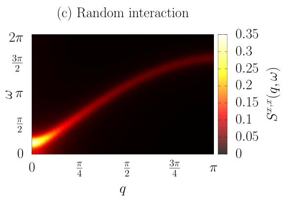
We will also study the case of random interactions and magnetic fields, related to lattice imperfections. In these cases the Hamiltonian takes the form in Eq. (21), but for the case of random interactions the Ising couplings take the form
| (23) |
for the short and long range models respectively. While in the case of random transverse fields
| (24) |
In all cases is drawn independently at random at each site, from a uniform distribution on the interval with , , , and . We employ between 50 and 100 disorder realizations per data point.
V Effect of experimental imperfections on the DSF of the short range TFIM
In the following, we will demonstrate that the qualitative and quantitative features of the DSF for both the short (and long range TFIM can be recovered from a quantum simulation even in the presence of experimental imperfections. Here, we discuss the role of imperfections and their impact as such; the certification of the actual correctness of the quantum simulation Eisert et al. is a separate task.
To phenomenologically and briefly summarize the results: We show that, at the experimental levels of control present in state of the art architectures, the errors which would be produced in a measurement of the DSF for both short and long range TFIM are small, and one can trust both the qualitative and quantitative results of such experiment. Since the overall behaviour of the DSF is what gives one information about low energy excitations of a given system, and how they behave, the errors studied show that, at the current level of experimental control (when our imperfection parameter is set below ), the DSF is well behaved. Thus, the overall form of the DSF does not change and one can safely extrapolate, from a quantum simulation via the DSF, what some of the low energy excitations of a given model are, and what their behaviour is.
V.1 Quantifying imperfections
To assess what the effect of experimental imperfections is on the DSF we will analyze two particular quantities based on the absolute error of the DSF. We define the absolute error as
| (25) |
where is the DSF obtained from the exact solution of the TFIM in the absence of imperfections. is the DSF obtained from the exact solution with various perturbations in the Hamiltonian, arising from the different imperfection models. If we integrate over frequency (reciprocal space) we obtain the average error in reciprocal space (frequency),
| (26) |
where is the number of frequencies, which depends on the discretization of the time evolution, and is the system size. We show the average error for different imperfection models in the supplementary information. The maximum of the absolute error, for fixed or , will be denoted by
| (27) |
These errors can be understood in the following way: (25) is the absolute error of the DSF when imperfections are considered. If one makes a cut on the absolute error at a given value of reciprocal space, , and integrates it over frequency, one obtains the frequency integrated error, . This is equivalent for cuts at a given frequency , to obtain . If, on the other hand, one selects the maximal error at that value, one obtains (27). The study of the imperfections in this way allows us to account for the effects in frequency and reciprocal space separately. If the imperfection models do not change the DSF, then these errors should be small and flat over the entire and range. On the other hand, if these errors are not small, we can assess what their effect is on the DSF by studying the shape of the quantities given in (26) and (27). For example, if one of these imperfection models were to close the gap, we would see errors towards small frequencies, but not on -space.
Since the Fourier transform is performed as data-processing over the correlators, we will compare the error of the DSF to the error in the correlators, as to assess the robustness of the Fourier transform. The error in the correlators, and the average and maximum over space (where space is indicated as ) are defined as
| (28) | ||||
| (29) |
Finally, to determine the scaling properties of the long range model, we will study the integrated DSF error as a function of size and of the range of the interactions where the integrated error is given by
| (30) |
V.2 Influence of state preparation imperfections on the DSF

We will concentrate on two architectures, trapped ions and Rydberg atom arrays. Both of them can prepare the initial state via an adiabatic evolution. Furthermore, trapped ions can prepare it through quantum approximate optimization techniques Pagano et al. 2019. We will study here how the DSF is affected by different evolution times, when the final field value is far away from the quantum critical point, and .
Adiabatic time evolution. The question that motivates us is how the features of the DSF change when the system is prepared for a time (the preparation time) from an initial polarized state, (which corresponds to the limit) to the final state . In the thermodynamic limit this preparation time diverges when one approaches the quantum critical point. For a finite system, it can be shown that the finite size gap destroys the divergence, and a finite bound on the preparation time can be obtained Dziarmaga 2005; Zurek et al. 2005 within which the evolution remains adiabatic.
Considering our previous discussion, it is imperative that we study how the properties of the DSF change when the preparation is not adiabatic. In this case, if the preparation time is not large enough to be in the adiabatic regime, the quantum simulation can still be able to obtain results which are close to the physics that one desires to study. This can be understood, and generalized to preparation protocols beyond adiabatic evolutions, in the context of prepared state fidelity. If the fidelity is high, then the properties of the DSF evaluated over the prepared state will remain close to the properties of the DSF evaluated over the exact ground state. Furthermore, if the preparation evolution is not adiabatic, but does not surpasses the quantum critical point, then there exists a time interval in which the transition probabilities towards excited states is sufficiently small, such that the main contribution to the state of the system is the ground state Dziarmaga 2005; Zurek et al. 2005; Cincio et al. 2007; Cincio et al. 2009; Kennes et al. 2018. At the parameter values studied here, the fidelity of the prepared state can be thought of as the probability that no extra domain walls (or equivalently, kinks) have been created during the preparation. Ref. Zurek et al. 2005 calculates the fidelity of the final state with respect to the vacuum of excitations for a linear ramp, effectively probing the probability that no excitations have been created during the preparation. The authors find that the fidelity takes the form
| (31) |
With this in mind, we can simply ask the question of how large does need to be such that , and what are the effects on the DSF when ?.
We quantify the robustness of the DSF to preparation imperfections employing the error measures shown in before. For this we numerically calculate the DSF of the short range TFIM,when we prepare the state by a total time , starting with the field at and finishing at .

The adiabatic evolution has been performed for different evolution times, ranging from to . In Fig. 5 we show the error analysis for preparation times , , , and . Following the calculations of Ref. Zurek et al. 2005 we estimate that the fidelity of the prepared state (assuming no other error sources) will correspond to for a preparation time of , to for , and for . Our numerical error analysis of the DSF and correlators coincides with these fidelity estimates. We tackle the DSF first: in the left most panel of Fig. 5 we show a typical DSF for a preparation time , and in the right most panel we show the maximum error of the DSF over frequency (main figure) and reciprocal space (inset). For the maximum error is below and mostly flat over the entire space, indicating that this is enough to obtain an accurate DSF. This can be confirmed by comparing the left most panel of Fig. 5 and Fig. 2. From these figures we notice that the discrepancy in the DSF between the exact case and the one studied in this section appears around the point which corresponds to the position of the gap in the clean case. Even for , most of the error is constrained around the gap, indicating that the main contribution to the error in the DSF is a qualitative change in the overall broadness of the low low sector, even though the overall shape of the DSF does not change ( as is seen in the left most panel).
In the case of unequal time correlators, shown in the middle panel of Fig. 5, we see that the maximal (average in the inset) error in this case, for , is also below (), but we can see how the average error increases over time. While looking at the correlators directly could also be a way to study the ground state fluctuation of the system (given that the effect of the imperfections is small), the interpretation of the data as a function of time can be much more challenging, especially for long times. This can be understood by considering the propagation of errors as a function of time, which takes place with a maximal velocity consistent with the Lieb-Robinson bounds. We show in Fig.5 in the supplementary information the propagation of errors in the correlators as a function of time. With this in mind, we can note that the Fourier transform leading to the DSF allows one to account for all the spacial and temporal data of the correlators, as well as understand and deal with errors arising from this imperfection model in a much simpler way.
V.3 Influence of evolution imperfections on DSF
In trapped ions architectures, the spin-spin interactions are created by coupling the spin states to the normal modes of motion of the ions by laser beams Kim et al. 2010; Edwards et al. 2010 (see section I in the supplementary information), obtaining a coupling strength directly proportional to the Rabi frequency of the ions. The lasers employed present intensity and phase oscillations which can be currently controlled up to a certain threshold Schneider and Milburn 1998. This induces a variation of the Rabi frequencies across the chain, resulting in interactions which are not uniform over time along the chain.
Globally fluctuating Ising coupling. We will study the particular case in which the intensity fluctuations of the lasers directly induce periodic fluctuations of the spin-spin interactions. We will model these evolution imperfections by modulating the Ising coupling as in (23), with different amplitudes and frequencies .
In Fig. 6 we show the error analysis of the DSF and unequal time correlation functions for the case of modulated Ising couplings. We have studied a range of frequencies from to and intensities in the range . Here, where , a coupling intensity correspond to a fluctuation in the Ising coupling. Current experimental capabilities can constrain these parameters within the threshold Friedenauer et al. 2008.
The effects are mainly noticed as a function of the coupling . Concentrating on the error of the DSF shown in the left and right most panels of Fig. 6, we see that even the lowest coupling studied can induce a maximal error of in the DSF. The error is mostly concentrated around gap. Already for we see that small broad peaks appear for , while for the shape of the DSF is changed, as indicated by the large errors all along the frequency axis in the left most panel of Fig. 6. This can be understood by looking at the left most panel of Fig. 6, comparing it with Fig. 2. Besides the overall decrease in intensity, the low frequency shape of the two particle continuum has changed, giving the maximum in the right most panel of Fig. 6 at . There is also an increase of intensity at small for a range of frequencies up to .
In the case of the unequal time correlators, the middle panel of Fig. 6, the error intensity is much higher, with a maximum of at small times which decays to close to zero, except for . This is an artefact generated by the error propagation in a Lieb-Robinson cone. Even if the maximal error is small, there is an overall error which increases with time, which indicates that long measurement times lead to the propagation of errors and to an, in average, very large inaccuracy in the correlators. As for the case of preparation imperfections, the error in the correlators can make for a hard determination of the propagation of excitations through the system. The DSF allows us to study these effects even in the presence of imperfections, given that the errors in this quantity are localized close to the maxima, and the overall shape of the two particle continuum is minimally changed for small intensities of the fluctuating coupling.
It has to be pointed out, that for slightly higher intensities of the fluctuating coupling, even for , small changes in the DSF are seen both in the frequency and reciprocal space axis. This indicates that this imperfection model has to be dealt with carefully in an experimental setup, as small increases in can lead to appreciable effects in both the DSF and the unequal time correlators.
Lattice imperfections. In a Rydberg atom setup spin-spin interactions can be generated by applying a spin-dependent optical dipole-force (Zhang et al. 2017; Bernien et al. 2017) (see section I in the supplementary material ). Since the Rydberg atoms are not in the ground state once in the local trap, and the experiment is carried at a finite temperature, fluctuations in the atomic positions for each atom in each cycle of the experiment are introduced Zhang et al. 2017; Bernien et al. 2017, which will affect the Ising interaction (see Eq. (2) in the supplementary information). In a typical experiment the fluctuation of the position lead to a change in the Ising coupling between and Zhang et al. 2017; Bernien et al. 2017 from shot to shot. This can be empirically modelled as a random Ising interactions as in (23). On the other hand the Rabi frequency is also not uniform along the chain. Since this frequency gives rise to the transverse field, this type of evolution imperfection can be studied as a random transverse fields as in (24).
In a setup where ions are trapped by a linear Paul trap, spin-spin interactions can be obtained applying off-resonant laser beams Kim et al. 2010; Edwards et al. 2010. The Rabi frequency can also vary across the chain from shot to shot (see Eq. (3) in the supplementary material), inducing random Ising interactions.
For these cases, random transverse fields and Ising interactions, we show the results in the section II of the supplementary material, since they are very similar as those found for the preparation imperfections. In both cases we see that the majority of the imperfections are concentrated around the maximum of the DSF, where the gap is located. Strong random Ising interactions tend to close the gap, as can be seen in Figs.1 and 3(c) in the section II of the supplementary material. On the other hand, random transverse fields tend to open it (see Figs.3 and 4(d) in the supplementary material). In both these cases, for the experimentally tolerable imperfections of around , the errors in the DSF and correlators are both reduced, leading to no noticeable effects in the DSF. While the errors in the correlators (Figs.1 and 2 in the supplementary material) are also small, the average error increases with time. In this sense, long measurement times can lead to very large errors, rendering the results analyzed purely via correlation functions highly unreliable.
We note that the regime in which randomness is large is interesting in itself, as it offers the chance to directly probe the effect of random disorder in spin chains via time dependent observables, and the DSF in particular, in near term quantum devices.
VI Influence of experimental imperfections on the DSF of the long range TFIM
In the previous section we have assessed the accuracy of a DSF measurement for the short range TFIM using quantum simulators, and have shown that the DSF is well behaved in the presence of experimental imperfections even at large system sizes. Now, we will put forward the idea that quantum simulators can recover the DSF of long range models accurately for system sizes larger than state of the art classical simulations can treat. To show this, we will numerically study the long range TFIM in the presence of the same experimental imperfections as for the short range TFIM.
In Fig. 4 we show the DSF in the absence of imperfections for three different values of . In section IV of the supplementary material we show the results for , , and . Furthermore, in section V of the supplementary information we show the heat maps for the unequal time correlations with respect to the middle of the chain, . In the regime our results exhibit a particular signature in the DSF which has no dependence. For higher values of remnants of this behaviour are noticed, but an dependence is recovered. For we recover the cosine shaped two particle continuum. These results, especially the absence of -dependence for , indicates that the signatures of excitation confinement, which have been recently proposed Liu et al. 2019; Lerose et al. 2019; Verdel et al. 2019 can be observed in dynamical quantum simulators via the DSF employing our proposed method.
In section IV in the supplementary material we show a typical case for the the maximal error as a function of frequency (reciprocal space) Eq. (26) (Eq. (27)) in the case of random transverse fields. There we can see that the overall behaviour of the error is very similar to that for the short range TFIM. There is a large error around the gap, with small fluctuations at other values of for strong imperfections. For small imperfection levels () the error in the DSF is negligible, for all imperfections models, as it was found for the short range TFIM.
In Fig. 7 we show the integrated error (30) as a function of the interaction range for the models corresponding to evolution imperfections. Fig. 7(a) show the error for the case of laser intensity fluctuations, while Fig. 7(b) and (c) show the random fields and random interactions respectively. In both cases we see two regimes, where the error drastically changes for , while it stabilizes for . For the laser intensity fluctuations, the error monotonically increases in the first regime, and saturates in the second. On the other hand, the opposite behaviour is observed for the lattice imperfections, where the error decreases as a function of .
While the errors change as the value of is modified, at the imperfection levels present in the current architectures the integrated error is negligible, indicating that the DSF at all values of can be probed using these setups and the measurement would yield accurate results.
VI.1 System size scaling for long range models
Now we concentrate on the scaling properties of the DSF of the long range TFIM. We study system sizes ranging from to sites employing full exact diagonalization, and analyze how the integrated error changes with size. Since current architectures can simulate up to approximately 50 sites Zhang et al. 2017; Bernien et al. 2017, this is a playground in which the DSF can be employed to explore the potential of dynamical analogue quantum simulators. We show the scaling properties of the error for and . In Fig. 8 we show the integrated error originating from the evolution imperfections, as a function of system size, for the two aforementioned values of .
For imperfection levels below , the integrated error is relatively constant over the full range of system sizes studied here. When the imperfection level is reduced further, below ( within current experimental capabilities), it becomes negligible for all system sizes and interaction ranges. Our data suggests that the error remains constant and small at even the smallest sizes studied here, indicates that the integrated DSF error is intensive with respect to the system sizes, and as such we expect that the scaling properties will be maintained for larger chains. Furthermore, our data indicates that a dynamical quantum simulator can measure the DSF of the long range TFIM accurately, even in the presence of realistic experimental imperfections, for system sizes considerably bigger than what is currently achievable with numerical simulations, thus paving the way towards a practical quantum advantage.
VII Conclusions
In this work, we propose the observation of dynamical structure factors as a practical application of dynamical quantum simulators. We have shown that the BQP-hardness of general local Hamiltonian time evolution is inherited by the dynamical structure factor, suggesting that its efficient classical computation might be infeasible also for practically relevant instances. In this endeavour, we build on the measurement protocol of Ref. Knap et al. 2013 and tomographic ideas, allowing to measure the DSF in several different quantum architectures. These architectures include those of trapped ion, Rydberg atoms, cold atoms in optical lattices, and superconducting qubits.
To emphasize the feasibility of this approach, we study the robustness of the DSF against several meaningful models of experimental imperfections for the short and long range transverse field Ising model (TFIM). Our results for the short range TFIM indicate that the overall features of the DSF are preserved when one considers state of the art setups, their associated experimental imperfections, and the current level of control over them. For the long range model, we observe that the effects of imperfections at the current experimental levels and for the system sizes studied in this work do not change the DSF. We have brought our findings into contact with signatures of the exotic physics in the long range TFIM, in particular the confinement of excitations which has been recently reported. Unlike previous studies, we observe the signatures of confinement in both the DSF and correlators in equilibrium, i.e., without the need to quench the Hamiltonian, with equilibrium being a fundamental requirement of our proposed DSF measurement protocol. Following the study of these imperfections we carry out a system size scaling, which indicates that the errors of the DSF induced by these imperfections are controlled over the whole range of sizes – remaining small and constant. This indicates that for the imperfections considered in this work, a quantum simulation experiment with system sizes considerably bigger than what state of the art classical algorithms can achieve is expected to yield accurate results. We therefore argue that the measurement of DSFs in quantum simulators provides a useful tool to assess time dependent quantities of key importance in condensed matter physics, and further place quantum simulators into the realm of quantum technological devices Acin et al. 2018. We hope that the present work stimulates further assessments of this quantity in other physical contexts.
VIII Acknowledgements
M. L. B. wishes to thank Dante Kennes, Markus Heyl, David Luitz, Pedram Roushan, Pietro Silvi, Jan Carl Budich, Bela Bauer, and Thierry Giamarchi for fruitful discussions. J. E. acknowledges discussions with Holger Boche. This work has been supported by the ERC (TAQ), the Templeton Foundation, the FQXi, and the DFG (EI 519/14-1, EI 519/15-1, CRC 183, FOR 2724) and MATH+. This work has also received funding from the European Unions Horizon 2020 research and innovation programme under grant agreement No 817482 (PASQuanS). J. B. V. acknowledges funding from the European Union’s Horizon 2020 research and innovation programme under the Marie Skłodowska-Curie grant agreement Nº 754446 and UGR Research and Knowledge Transfer Found – Athenea3i.
References
- Foulkes et al. (2001) W. M. C. Foulkes, L. Mitas, R. J. Needs, and G. Rajagopal, Rev. Mod. Phys. 73, 33 (2001).
- Noack and Manmana (2005) R. M. Noack and S. R. Manmana, AIP Conf. Proc. 789, 93 (2005).
- Orus (2018) R. Orus, arXiv e-prints (2018), arXiv:1812.04011 .
- Aaronson (2005) S. Aaronson, arXiv e-prints (2005), arXiv:quant-ph/0502072 [quant-ph] .
- Aaronson (2009) S. Aaronson, (2009), arXiv:0910.4698 .
- Ran and Tal (2019) R. Ran and A. Tal, Proc. STOC 51st Ann. ACM SIGACT Symp. Th. Comp. , 13 (2019).
- Marvian et al. (2019) M. Marvian, D. A. Lidar, and I. Hen, Nature Comm. 10, 1571 (2019).
- (8) J. Klassen, M. Marvian, S. Piddock, M. Ioannou, I. Hen, and B. Terhal, arXiv:1906.08800 .
- Hangleiter et al. (2019) D. Hangleiter, I. Roth, D. Nagaj, and J. Eisert, arXiv e-prints (2019), arXiv:1906.02309 [quant-ph] .
- Cirac and Zoller (2012) J. I. Cirac and P. Zoller, Nature Phys. 8, 264 (2012).
- Eisert et al. (2015) J. Eisert, M. Friesdorf, and C. Gogolin, Nature Phys. 11, 124 (2015).
- Fukuhara et al. (2013a) T. Fukuhara, P. Schauß, M. Endres, S. Hild, M. Cheneau, I. Bloch, and C. Gross, Nature 502, 76 (2013a).
- Fukuhara et al. (2013b) T. Fukuhara, A. Kantian, M. Endres, M. Cheneau, P. Schauß, S. Hild, D. Bellem, U. Schollwöck, T. Giamarchi, C. Gross, I. Bloch, and S. Kuhr, Nature Phys. 9, 235 (2013b).
- Cheneau et al. (2012) M. Cheneau, P. Barmettler, D. Poletti, M. Endres, P. Schauß, T. Fukuhara, C. Gross, I. Bloch, C. Kollath, and S. Kuhr, Nature 481, 484 (2012).
- Simon et al. (2011) J. Simon, W. S. Bakr, R. Ma, M. E. Tai, P. M. Preiss, and M. Greiner, Nature 472, 307 (2011).
- Bernien et al. (2017) H. Bernien, S. Schwartz, A. Keesling, H. Levine, A. Omran, H. Pichler, S. Choi, A. S. Zibrov, M. Endres, M. Greiner, V. Vuletić, and M. D. Lukin, Nature 551, 579 (2017).
- Zhang et al. (2017) J. Zhang, G. Pagano, P. W. Hess, A. Kyprianidis, P. Becker, H. Kaplan, A. V. Gorshkov, Z. X. Gong, and C. Monroe, Nature 551, 601 (2017).
- Bohnet et al. (2016) J. G. Bohnet, B. C. Sawyer, J. W. Britton, M. L. Wall, A. M. Rey, M. Foss-Feig, and J. J. Bollinger, Science 352, 1297 (2016).
- Islam et al. (2011) R. Islam, E. E. Edwards, K. Kim, S. Korenblit, C. Noh, H. Carmichael, G. D. Lin, L. M. Duan, C. C. Joseph Wang, J. K. Freericks, and C. Monroe, Nature Comm. 2, 377 (2011).
- Trotzky et al. (2012) S. Trotzky, Y.-A. Chen, A. Flesch, I. P. McCulloch, U. Schollwöck, J. Eisert, and I. Bloch, Nature Phys. 8, 325 (2012).
- Coldea et al. (2010) R. Coldea, D. A. Tennant, E. M. Wheeler, E. Wawrzynska, D. Prabhakaran, M. Telling, K. Habicht, P. Smeibidl, and K. Kiefer, Science 327, 177 (2010).
- Jia et al. (2014) C. J. Jia, E. A. Nowadnick, K. Wohlfeld, Y. F. Kung, C. C. Chen, S. Johnston, T. Tohyama, B. Moritz, and T. P. Devereaux, Nature Comm. 5, 3314 (2014).
- Sachdev (2011) S. Sachdev, Quantum phase transitions, 2nd ed. (Cambridge University Press, 2011).
- Roushan et al. (2017) P. Roushan, C. Neill, J. Tangpanitanon, V. M. Bastidas, A. Megrant, R. Barends, Y. Chen, Z. Chen, B. Chiaro, A. Dunsworth, A. Fowler, B. Foxen, M. Giustina, E. Jeffrey, J. Kelly, E. Lucero, J. Mutus, M. Neeley, C. Quintana, D. Sank, A. Vainsencher, J. Wenner, T. White, H. Neven, D. G. Angelakis, and J. Martinis, Science 358, 1175 (2017).
- Barredo et al. (2015) D. Barredo, H. Labuhn, S. Ravets, T. Lahaye, A. Browaeys, and C. S. Adams, Phys. Rev. Lett. 114, 113002 (2015).
- Liu et al. (2019) F. Liu, R. Lundgren, P. Titum, G. Pagano, J. Zhang, C. Monroe, and A. V. Gorshkov, Phys. Rev. Lett. 122, 150601 (2019).
- Luitz and Bar Lev (2019) D. J. Luitz and Y. Bar Lev, Phys. Rev. A 99, 010105(R) (2019).
- Fratus and Srednicki (2016) K. R. Fratus and M. Srednicki, (2016), arXiv:1611.03992 .
- Hauke and Tagliacozzo (2013) P. Hauke and L. Tagliacozzo, Phys. Rev. Lett. 111, 207202 (2013).
- Knap et al. (2013) M. Knap, A. Kantian, T. Giamarchi, I. Bloch, M. D. Lukin, and E. Demler, Phys. Rev. Lett. 111, 147205 (2013).
- Yoshimura and Freericks (2016) B. T. Yoshimura and J. K. Freericks, Phys. Rev. A 93, 052314 (2016).
- Pagano et al. (2019) G. Pagano, A. Bapat, P. Becker, K. S. Collins, A. De, P. W. Hess, H. B. Kaplan, A. Kyprianidis, W. L. Tan, C. Baldwin, L. T. Brady, A. Deshpande, F. Liu, S. Jordan, A. V. Gorshkov, and C. Monroe, arXiv e-prints , arXiv:1906.02700 (2019), arXiv:1906.02700 [quant-ph] .
- Baiesi et al. (2009) M. Baiesi, C. Maes, and B. Wynants, Phys. Rev. Lett. 103, 010602 (2009).
- Calzetta and Hu (2008) E. A. Calzetta and B.-L. B. Hu, Nonequilibrium quantum field theory (2008).
- Boche and Mönich (2019) H. Boche and U. J. Mönich, (2019), in preparation.
- Kempe et al. (2004) J. Kempe, A. Kitaev, and O. Regev, SIAM J. Comp. 35, 1070 (2004).
- Gosset et al. (2015) D. Gosset, B. M. Terhal, and A. Vershynina, Phys. Rev. Lett. 114, 140501 (2015).
- Lloyd and Terhal (2016) S. Lloyd and B. M. Terhal, New J. Phys. 18, 023042 (2016).
- Ciani et al. (2019) A. Ciani, B. Terhal, and D. DiVinzenzo, Quant. Sc. Tech. 4, 035002 (2019).
- Lerose et al. (2019) A. Lerose, B. Žunkovič, A. Silva, and A. Gambassi, Phys. Rev. B 99, 121112(R) (2019).
- Derzhko and Krokhmalskii (1997) O. Derzhko and T. Krokhmalskii, Phys. Rev. B 56, 11659 (1997).
- Saadatmand et al. (2018) S. N. Saadatmand, S. D. Bartlett, and I. P. McCulloch, Phys. Rev. B 97, 155116 (2018).
- Crosswhite et al. (2008) G. M. Crosswhite, A. C. Doherty, and G. Vidal, Phys. Rev. B 78, 035116 (2008).
- Haegeman et al. (2011) J. Haegeman, J. I. Cirac, T. J. Osborne, I. Pižorn, H. Verschelde, and F. Verstraete, Phys. Rev. Lett. 107, 070601 (2011).
- Zaletel et al. (2015) M. P. Zaletel, R. S. K. Mong, C. Karrasch, J. E. Moore, and F. Pollmann, Phys. Rev. B 91, 165112 (2015).
- Hashizume et al. (2018) T. Hashizume, I. P. McCulloch, and J. C. Halimeh, arXiv e-prints (2018), arXiv:1811.09275 .
- Buyskikh et al. (2016) A. S. Buyskikh, M. Fagotti, J. Schachenmayer, F. Essler, and A. J. Daley, Phys. Rev. A 93, 053620 (2016).
- Hastings and Koma (2006) M. B. Hastings and T. Koma, Commun. Math. Phys. 265, 781 (2006).
- Verdel et al. (2019) R. Verdel, F. Liu, S. Whitsitt, A. V. Gorshkov, and M. Heyl, arXiv e-prints (2019), arXiv:1911.11382 .
- (50) J. Eisert, D. Hangleiter, N. Walk, I. Roth, D. Markham, R. Parekh, U. Chabaud, and E. Kashefi, ArXiv:1910.06343, arXiv:arXiv:1910.06343 .
- Dziarmaga (2005) J. Dziarmaga, Phys. Rev. Lett. 95, 245701 (2005).
- Zurek et al. (2005) W. H. Zurek, U. Dorner, and P. Zoller, Phys. Rev. Lett. 95, 105701 (2005).
- Cincio et al. (2007) L. Cincio, J. Dziarmaga, M. M. Rams, and W. H. Zurek, Phys. Rev. A 75, 052321 (2007).
- Cincio et al. (2009) L. Cincio, J. Dziarmaga, J. Meisner, and M. M. Rams, Phys. Rev. B 79, 094421 (2009).
- Kennes et al. (2018) D. M. Kennes, C. Karrasch, and A. J. Millis, arXiv e-prints (2018), arXiv:1809.00733 .
- Kim et al. (2010) K. Kim, M. S. Chang, S. Korenblit, R. Islam, E. E. Edwards, J. K. Freericks, G. D. Lin, L. M. Duan, and C. Monroe, Nature 465, 590 (2010).
- Edwards et al. (2010) E. E. Edwards, S. Korenblit, K. Kim, R. Islam, M.-S. Chang, J. K. Freericks, G.-D. Lin, L.-M. Duan, and C. Monroe, Phys. Rev. B 82, 060412(R) (2010).
- Schneider and Milburn (1998) S. Schneider and G. J. Milburn, Phys. Rev. A 57, 3748 (1998).
- Friedenauer et al. (2008) A. Friedenauer, H. Schmitz, J. T. Glueckert, D. Porras, and T. Schaetz, Nature Phys. 4, 757 (2008).
- Acin et al. (2018) A. Acin, I. Bloch, H. Buhrman, T. Calarco, C. Eichler, J. Eisert, D. Esteve, N. Gisin, S. J. Glaser, F. Jelezko, S. Kuhr, M. Lewenstein, M. F. Riedel, P. O. Schmidt, R. Thew, A. Wallraff, I. Walmsley, and F. K. Wilhelm, New J. Phys. 20, 080201 (2018).
- Schauss (2018) P. Schauss, Quant. Sc. Tech. 3, 023001 (2018).
- Schneider et al. (2012) C. Schneider, D. Porras, and T. Schaetz, Rep. Prog. Phys. 75, 024401 (2012).
Appendix A Platforms considered
A.1 Rydberg atoms
For a Rydberg atoms setup, we consider the case of an array of trapped cold neutral 70S atoms with strong, controllable interactions. In this case, the atoms are trapped by optical tweezers, and the state of the art architecture can contain up to 51 atomsBernien et al. 2017. A two-photon process couples the ground state vector to a target Rydberg state vector of the Rb atoms via an intermediate state. This transition is driven by two lasers detuned from the Rydberg state. The dynamics of the system is given by (Zhang et al. 2017; Bernien et al. 2017)
| (32) |
where is a detuning factor away from the Rydberg state, is the Rabi frequency of the atom at the th position, is the coupling between the ground state and Rydberg state, and . The interaction strength elements can also be tuned by varying the distance between them or by coupling them to a different Rydberg state. To transform this Hamiltonian into an transverse field Ising model Schauss 2018 we just need to identify at each site , and such that and , with . Replacing in the Hamiltonian, we obtain a transverse field Ising model with a coupling of the form
| (33) |
The longitudinal field in the above expression can be suppressed by the detuning factor . The Ising interaction arises from van der Waals interactions between the atoms when they are both in the Rydberg state, and takes the form , with . As such, since the Rydberg atoms are not in the ground state once in the local trap, and the experiment is carried at a finite temperature, fluctuations in the atomic positions for each atom in each cycle of the experiment are introduced Zhang et al. 2017; Bernien et al. 2017. This will affect the Ising interaction, Eq. (33). We finally note that the mean lifetime of a chain scales inversely with the number of ions, with an average of 5 minutes for a chain of 53 ions.
A.2 Trapped ions
We will consider here a particular trapped ion setup, where are trapped by a linear Paul trap. A 1D spin-1/2 Ising system in the presence of a transverse field can be engineered Islam et al. 2011 by the hyperfine ”clock” states and which represent the and eigenstates of and are sparated by . These ions are trapped by a linear Paul trap, and their modes of motion are cooled near the ground state. The transverse field and spin-spin interactions can be obtained applying off-resonant laser beams Kim et al. 2010; Edwards et al. 2010. A transverse field can be generated by uniformly illuminating the ion chain with two Raman laser beams whose difference in frequency is tuned to the hyperfine splitting . This induces Rabi oscillations in the ions which are seen as AC Stark shifts in the spin states. On the other hand, the spin-spin interactions are created by coupling the spin states to the normal modes of motion of the ions by the Raman beams. The beams are made to carry beat note at frequencies , which generates a spin-dependent force at frequency Schneider et al. 2012. As such, controlling the beat note frequency , one can generate Ising interactions with a coupling given by
| (34) |
where is the Rabi frequency of the th ion, is the Lamb-Dicke parameter of the th mode of the th ion at frequency , and the assumption of indicating that only virtual phonons are excited. These interactions are not necessarily uniform, since the Rabi frequency can vary across the chain and other vibrational models can also contribute considerably. Furthermore, by tuning one can tune between .
Appendix B Numerical results for position fluctuations and random fields of Rydberg atoms
Appendix C Dynamical structure factors for the short range transverse field Ising



Appendix D Dynamical structure factors for the long range transverse field Ising


Appendix E Unequal time correlation function for the long range transverse field Ising


Appendix F Numerical results for position fluctuations in the long range TFIM

